Laplacian growth in the half plane

We investigate a version of the Laplacian growth problem with zero surface tension in the half plane and find families of self-similar exact solutions.

1 Introduction

In this paper we find some self-similar exact solutions of the following version of the Laplacian growth problem in the half plane ℍ introduced in [1]. Let $\gamma$ be a smooth non-self-intersecting curve in ℍ from a point $x_{-}\in\mbox{\Bbb R}$ to a point $x_{+}\in\mbox{\Bbb R}$ (we assume that $x_{-}\leq x_{+}$) and ${\sf B}$ be the domain bounded by this curve and the segment $[x_{-},x_{+}]$ of the real axis. (In [1] such domains are called fat slits.) Suppose the curve $\gamma=\gamma(T)$ moves with time $T$ according to the Darcy law:

$$V_{n}(z)=\frac{1}{2}\,\partial_{n}\phi(z)\,,\quad z\in\gamma\,.$$ (1)

Here $\partial_{n}$ is the normal derivative at the boundary, with the outward looking normal vector, $V_{n}(z)$ is the normal velocity at the point $z\in\gamma$ and $\phi$ is a unique harmonic function in $\mbox{\Bbb H}\setminus{\sf B}$ such that

• $\phi=0$ on $\gamma$ and on the rays of the real axis $[-\infty,x_{-}]$, $[x_{+},+\infty]$;

• $\phi(z)={\cal I}m\,z+o(1)$ as ${\cal I}m\,z\to+\infty$.

As is argued in [1], the growth process is well defined if both angles $\alpha_{\pm}$ between $\gamma$ and the real axis at the points $x_{\pm}$ are acute. Then these angles as well as the points $x_{-}$, $x_{+}$ stay fixed all the time.

Comparing this setting with the standard Laplacian growth in the upper half plane (see, e.g., [2]), we see that the conditions on the harmonic function $\phi$ are very similar: $\phi=0$ on an infinite contour from left to right infinity and becomes ${\cal I}m\,z$ as ${\cal I}m\,z\to+\infty$. An important difference is that in our case, unlike in the standard one, only a finite part of the level line $\phi=0$ (namely, the part which lies above the real axis) moves according to the Darcy law while the remaining part (the rays of the real axis) is kept fixed despite the fact that the gradient of $\phi$ is nonzero there.

It is often convenient to treat the growing domain ${\sf B}$ as an upper half of the domain ${\sf D}={\sf B}\cup\bar{\sf B}$ symmetric with respect to the real axis, with the boundary $\Gamma=\gamma\cup\bar{\gamma}$. Here $\bar{\sf B}$ is the domain in the lower half plane obtained from ${\sf B}$ by complex conjugation $z\to\bar{z}$. In what follows we call such domains simply symmetric. Then one can extend the problem (1) to the whole plain “by reflection”, i.e., by saying that $V_{n}(z)=\frac{1}{2}\,\partial_{n}\phi(z)$ for $z\in\gamma$ and $V_{n}(z)=-\frac{1}{2}\,\partial_{n}\phi(z)$ for $z\in\bar{\gamma}$, where $\phi$ is a harmonic function in $\mbox{\Bbb C}\setminus{\sf D}$ such that (i) $\phi(\bar{z})=-\phi(z)$; (ii) $\phi=0$ on $\Gamma=\gamma\cup\bar{\gamma}$; (iii) $\phi(z)={\cal I}m\,z+o(1)$ as ${\cal I}m\,z\to\pm\infty$.

2 Formulation in terms of conformal maps

As is customary in moving boundary problems, we reformulate the problem in terms of time-dependent conformal maps to (or from) some fixed reference domain from (or to) the domain $\mbox{\Bbb C}\setminus{\sf D}(T)$, where the Laplace equation is to be solved. In our case there are two distinguished choices of the reference domain: the upper half plane and the exterior of the unit circle.

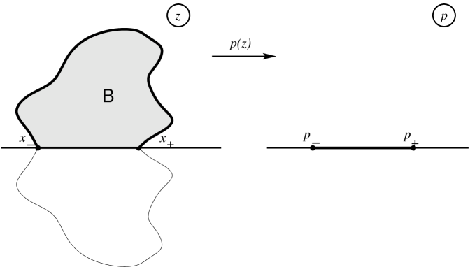
Figure 1: The conformal map $p(z)$. The mirror image of the domain ${\sf B}$ in the lower half-plane is also shown.

The upper half plane.

This choice is natural when one deals with the original formulation of the problem in the upper half plane not extending it to the lower one by reflection. Let $p(z)$ be a conformal map from $\mbox{\Bbb H}\setminus{\sf B}$ (in the “physical” $z$-plane) onto ℍ (in the “mathematical” $p$-plane) shown schematically in Fig. 1. We normalize it by the condition that the expansion of $p(z)$ in a Laurent series at infinity is of the form

$$p(z)=z+\frac{u_{1}}{z}+\sum_{k\geq 2}u_{k}z^{-k}\,,\quad|z|\to\infty$$ (2)

(a “hydrodynamic” normalization). Assuming this normalization, the map is unique. The upper part of the boundary, $\gamma$, is mapped to a segment of the real axis $[p_{-},\,p_{+}]$, while the rays of the real axis outside ${\sf B}$ are mapped to the real rays $[-\infty,\,p_{-}]$ and $[p_{+},\,\infty]$. From this it follows that the coefficients $u_{k}$ are all real numbers. The first coefficient, $u_{1}$, is called a capacity of ${\sf B}$. It is known to be positive. We also need the inverse map, $z(p)$, which can be expanded into the inverse Laurent series

$$z(p)=p-\frac{u_{1}}{p}+\sum_{k=2}^{\infty}a_{k}p^{-k}\,,\quad|p|\to\infty$$ (3)

with real coefficients $a_{k}$ connected with $u_{k}$ by polynomial relations. The series converges for large enough $|p|$.

Clearly, the harmonic function ${\cal I}m\,p(z)$ obeys all the conditions required from the $\phi(z)$, so $\phi(z)={\cal I}m\,p(z)$. It is easy to see that $\partial_{n}{\cal I}m\,p(z)=|p^{\prime}(z)|$ on $\gamma$, so one can write the Darcy law as $V_{n}(z)=\frac{1}{2}|p^{\prime}(z)|$.

The Schwarz symmetry principle allows one to extend this reformulation to the whole plane as follows. The function $z(p)$ admits an analytic continuation to the lower half plane as $\overline{z(\bar{p})}$. The analytically continued function performs a conformal map from the whole complex plane with a cut on the real axis between $p_{-}$ and $p_{+}$ onto the exterior of the symmetric domain ${\sf D}={\sf B}\cup\bar{\sf B}$. Correspondingly, the inverse function, $p(z)$, obeys $p(\bar{z})=\overline{p(z)}$ and $\partial_{n}{\cal I}m\,p(z)=-|p^{\prime}(z)|$ on $\bar{\gamma}$. The evolution of the whole closed contour $\Gamma=\gamma\cup\bar{\gamma}$ can then be written in a unified way as $V_{n}(z)=\frac{1}{2}|p^{\prime}(z)|$ for any $z\in\Gamma$.

The map $z(p)$ plays a crucial role in the embedding of the problem into the dispersionless KP hierarchy found in [1] but appears to be rather inconvenient for constructing explicit solutions. This is certainly related to the fact that the symmetrically extended reference domain in the mathematical plane is singular (plane with a cut) and, moreover, depends on time. There is another choice of reference domain which seems to be less natural from the point of view of integrable hierarchies but is more suitable for finding explicit solutions.

The exterior of the unit circle.

In this case it is convenient to work with symmetrically extended domains from the very beginning. Let $f(w)$ be the conformal map from the exterior of the unit circle onto the exterior of the symmetric domain ${\sf D}$ such that $f(\infty)=\infty$ and $f^{\prime}(\infty)=r>0$, so that the Laurent expansion at $\infty$ has the form $f(w)=rw+u_{0}+O(w^{-1})$ with real coefficients. The coefficient $r$ is called the (external) conformal radius of the domain ${\sf D}$. The connection with the previously considered map is as follows: let $w(z)$ be the inverse function, then $p(z)=r(w(z)+w^{-1}(z))+u_{0}$ with $r=\frac{1}{4}(p_{+}-p_{-})$ and $u_{0}=\frac{1}{2}(p_{+}+p_{-})$.

Let us rewrite the Darcy law as a dynamical equation for the function $f(w)=f(w,T)$. To do that, we need the following simple kinematical relation which can be derived in a direct way. Let $z(\sigma,T)=x(\sigma,T)+iy(\sigma,T)$ be any parametrization of the contour such that $\sigma$ is a steadily increasing function of the arc length, then

$$V_{n}=\frac{d\sigma}{dl}(\partial_{T}x\partial_{\sigma}y-\partial_{T}y\partial_{\sigma}x)=\frac{d\sigma}{2idl}(\partial_{T}\bar{z}\partial_{\sigma}z-\partial_{T}z\partial_{\sigma}\bar{z})\,,$$ (4)

where $dl=|dz|=\sqrt{(dx)^{2}+(dy)^{2}}$ is the line element along the contour. According to our convention, $V_{n}(z)$ is positive when the contour, in a neighborhood of the point $z$, moves to the right of the increasing $\sigma$ direction. Set $\sigma=-i\log w$, $z=f(w,T)$, $\bar{z}=f(1/w,T)$, then the kinematical formula gives

$$V_{n}(f(w))=\frac{dw}{2i|df(w)|}\Bigl{(}\partial_{T}f(1/w)\partial_{w}f(w)-\partial_{T}f(w)\partial_{w}f(1/w)\Bigr{)}\,,\quad|w|=1$$

On the other hand, the Darcy law reads

$$V_{n}(f(w))=\frac{1}{2}\,\frac{|dp/dw|}{|df/dw|}\,,\quad\quad|w|=1$$

Equating the right hand sides and using the relation $dp/dw=r(1-w^{-2})$, we get the equation

$$w\partial_{w}f(w)\partial_{T}f(1/w)-w\partial_{w}f(1/w)\partial_{T}f(w)=r\left|w\!-\!w^{-1}\right|\,,\quad|w|=1$$ (5)

which is the main dynamical equation of the problem in terms of the conformal map.

It is instructive to compare it with the similar equation for the Laplacian growth process in the whole plane (i.e., without the condition that $\phi$ vanishes on the the real axis) and with the same type of source at infinity. In the latter case the evolution necessarily destroys the reflection symmetry, so the function $f(1/w)$ should be replaced by $\bar{f}(1/w)\equiv\overline{f(1/\bar{w})}$ while the form of the r.h.s. should be also changed to $-ir(w-w^{-1})$.

For finding explicit solutions of prime importance is the case when the function $f(w,T)$ admits an analytic continuation across the unit circle for all $T$ in some time interval, so that $f(w,T)$ is actually analytic not only in its exterior but in some larger domain containing it. However, one should take into account that such a continuation is impossible through the points $w=\pm 1$ which are pre-images of the two corner points and so $f(w)$ is not analytic there. Assuming that it is analytic everywhere else on the unit circle, one can analytically continue equation (5) as follows:

$$w\partial_{w}f(w)\partial_{T}f(1/w)-w\partial_{w}f(1/w)\partial_{T}f(w)=\left\{\begin{array}[]{l}-ir(w-w^{-1})\,,\quad{\cal I}m\,w>0\\ \\ \,\,\,ir(w-w^{-1})\,,\quad{\cal I}m\,w<0\end{array}\right.$$ (6)

Note that the analytic continuations to the upper and lower half planes are different.

3 Formulation in terms of Schwarz function

It is known [2] that the standard Laplacian growth problem in the whole plane can be integrated in terms of the Schwarz function. For analytic contours, the Schwarz function $S(z)$ is defined as the analytic continuation of the function $\bar{z}$ away from the contour. In other words, the Schwarz function for a curve $\Gamma$ is an analytic function $S(z)$ such that $\bar{z}=S(z)$ for $z\in\Gamma$ (see [3] for details). If the curve depends on time, so does its Schwarz function, $S=S(z,T)$.

In our problem the contour $\Gamma$ is not analytic because it always contains the two corner points. However, if the curve $\gamma$ is analytic, its Schwarz function, which we still denote by $S(z)$, is well defined in a strip-like neighborhood of the curve, with the width of the strip tending to zero around the endpoints $x_{\pm}$. We thus have $\bar{z}=S(z)$ for $z\in\gamma$ or, equivalently, $\bar{z}=\overline{S(\bar{z})}$ for $z\in\bar{\gamma}$. The latter formula just means that $\bar{S}(z)=\overline{S(\bar{z})}$ is the Schwarz function for the complex conjugate curve $\bar{\gamma}$. Therefore, we can expect that our problem can be integrated in terms of two Schwarz functions, $S(z)$ and $\bar{S}(z)$, enjoying equal rights. Below, just for brevity, the pair $(S(z),\bar{S}(z))$ is referred to as the Schwarz function of the piecewise analytic contour $\Gamma=\gamma\cup\bar{\gamma}$. In the mathematical $w$-plane, the role of the Schwarz function is to connect $f(w)$ and $f(1/w)$ in their common domains of analyticity:

$$f(w)=\left\{\begin{array}[]{l}\bar{S}(f(1/w))\,,\quad{\cal I}m\,w>0\\ \\ S(f(1/w))\,,\quad{\cal I}m\,w<0\end{array}\right.$$ (7)

Note that the second equality (at ${\cal I}m\,w<0$) is obtained from the first one by complex conjugation.

In complete analogy with the Laplacian growth problem in the whole plane, the growth process (1) is encoded in the equation $i\partial_{T}S=\partial_{z}p$ in the upper half plane. Extending it to the lower half plane by reflection (i.e., complex conjugation), we have, for all $z\in\mbox{\Bbb C}\setminus{\sf D}(T)$:

$$\left\{\begin{array}[]{l}i\partial_{T}S(z,T)\,=\,\partial_{z}p(z,T)\,,\quad{\cal}Im\,z>0\\ \\ i\partial_{T}\bar{S}(z,T)=-\partial_{z}p(z,T)\,,\quad{\cal}Im\,z<0\end{array}\right.$$ (8)

It is convenient to rewrite the above relations in terms of the piecewise analytic function

$$M(z)=\left\{\begin{array}[]{l}\,\,i(S(z)\,-\,z),\quad{\cal}Im\,z>0\\ \\ -i(\bar{S}(z)-z),\quad{\cal}Im\,z<0\end{array}\right.$$ (9)

introduced in [1]. By construction, it provides the analytic continuation of the function $2|{\cal I}m\,z|$ away from the contour $\Gamma$. Equivalently, we write $S(z)=z-iM(z)$ for ${\cal}Im\,z>0$ and $\bar{S}(z)=z+iM(z)$ for ${\cal}Im\,z<0$ or, passing to the mathematical $w$-plane,

$$f(w)=\left\{\begin{array}[]{l}f(1/w)+iM(f(1/w))\,,\quad{\cal I}m\,w>0\\ \\ f(1/w)-iM(f(1/w))\,,\quad{\cal I}m\,w<0\end{array}\right.$$ (10)

In terms of the function $M=M(z,T)$ the dynamical equation (8) acquires the form

$$\partial_{T}M(z,T)=\partial_{z}p(z,T)$$ (11)

Note that the function $\partial_{z}p(z,T)$ is holomorphic in $\mbox{\Bbb C}\setminus{\sf D}(T)$ with the expansion $\partial_{z}p(z,T)=1+O(1/z^{2})$ at infinity.

The function $M(z)$ can be uniquely decomposed as $M(z)=M_{+}(z)-M_{-}(z)$, where $M_{+}$ is analytic in ${\sf D}$ and $M_{-}$ is analytic in $\mbox{\Bbb C}\setminus{\sf D}$ with zero at infinity. This decomposition is given by the integral of Cauchy type

$$M_{+}(z)=\frac{1}{2\pi i}\oint_{\partial{\sf D}}\frac{M(z^{\prime})\,dz^{\prime}}{z^{\prime}-z}=\frac{1}{\pi i}\oint_{\partial{\sf D}}\frac{|{\cal I}m\,z^{\prime}|\,dz^{\prime}}{z^{\prime}-z}\,,\quad z\in{\sf D}$$ (12)

(and the same integral for $M_{-}(z)$ with $z$ outside ${\sf D}$). The function $M_{+}$ is analytic everywhere in ${\sf D}$ and, by our assumption, can be analytically continued across the arcs $\gamma$ and $\bar{\gamma}$ everywhere except for their endpoints on the real axis, where it has a singularity. One can see that the function $M_{+}(z)$ is the generating function of integrals of motion for our problem. Indeed, it is straightforward to calculate its time derivative:

$$\partial_{T}M_{+}(z)=\frac{1}{\pi i}\oint_{\partial{\sf D}}\frac{\mbox{sign}({\cal I}m\,z^{\prime})V_{n}(z^{\prime})}{z-z^{\prime}}\,|dz^{\prime}|\,,$$ (13)

(see [1] for details). Plugging here $V_{n}(z)=\frac{1}{2}|p^{\prime}(z)|$ and recalling that $dp(z)$ is purely real on $\Gamma$, we obtain

$$\partial_{T}M_{+}(z)=\frac{1}{2\pi i}\oint_{\partial{\sf D}}\frac{dp(z^{\prime})}{z^{\prime}-z}=1$$

where only the residue at infinity contributes because $p^{\prime}(z)$ is holomorphic in the exterior of ${\sf D}$ and $z$ is inside. Therefore, we have obtained the important equation

$$\partial_{T}M_{+}(z,T)=1$$ (14)

which allows one to construct an infinite series of integrals of motion by expanding $M_{+}(z)$ into a series in $z$.

In the case of general position, when $x_{-}\neq x_{+}$, one may expand $M_{+}(z)$ in a Taylor series around a point on the real axis lying inside ${\sf D}$ on the segment $[x_{-},x_{+}]$. Choosing the coordinate in such a way that $x_{-}<0<x_{+}$, one can expand around the origin:

$$M_{+}(z)=T+\sum_{k=2}^{\infty}kT_{k}z^{k-1}.$$ (15)

Equation (14) shows that the coefficients $T_{k}$, $k\geq 2$, are conserved: $\partial_{T}T_{k}=0$. They are the following harmonic moments of the domain $\mbox{\Bbb H}\setminus{\sf B}$:

$$T_{k}=\frac{1}{\pi ik}\oint_{{\sf D}}|{\cal I}m\,z|z^{-k}dz=\frac{2}{\pi k}\int_{\mbox{\Bbbb H}\setminus{\sf B}}\!{\cal I}m\left(z^{-k}\right)d^{2}z\,,\quad k\geq 2$$ (16)

One may also consider degenerate configurations with $x_{-}=x_{+}=0$. In this case the function $M_{+}(z)-T$ is still conserved but can not be represented by a Taylor series around the origin, and so the moments (16) are ill-defined.

4 Self-similar solutions

Self-similar solutions are characterized by the property

$$f(w,T)=r(T)f(w)$$ (17)

which means that the time evolution is equivalent to a dilatation in the $z$-plane. Because the time evolution is always such that the points $x_{\pm}$ stay fixed, self-similar solutions have chance to exist only when $x_{-}=x_{+}=0$ which is just the degenerate case mentioned at the end of the previous section. Exact self-similar solutions of Laplacian growth in radial and wedge geometries were studied in [4]-[9].

4.1 General relations

Differential equation for $f(w)$.

Substituting the self-similar ansatz (17) into (6), we see that the variables separate: $r(T)=T/A$ and

$$w\partial_{w}f(w)f(1/w)-w\partial_{w}f(1/w)f(w)=A\left\{\begin{array}[]{l}-i(w-w^{-1})\,,\quad{\cal I}m\,w>0\\ \\ \,\,\,i(w-w^{-1})\,,\quad{\cal I}m\,w<0\end{array}\right.$$

where $A$ is a constant. This latter equation can be treated as the Wronskian relation for a second order differential equation of the form

$$A_{2}(w)\psi^{\prime\prime}+A_{1}(w)\psi^{\prime}+A_{0}(w)\psi=0$$

Namely, let $\psi_{1}$, $\psi_{2}$ be two linearly independent solutions, then their Wronsky determinant, $W=\psi_{1}\psi_{2}^{\prime}-\psi_{2}\psi_{1}^{\prime}$ obeys the relation

$$\partial_{w}\log W(w)=-\,\frac{A_{1}(w)}{A_{2}(w)}$$

In our case $W=\pm iA(1-w^{-2})$, so $\displaystyle{\partial_{w}\log W=\frac{1}{w+1}+\frac{1}{w-1}-\frac{2}{w}}$ (note that this expression is the same in the both half planes) and the functions $f(w)$ and $f(1/w)$ are two solutions of the ordinary differential equation

$$\partial_{w}^{2}f-\left(\frac{1}{w+1}+\frac{1}{w-1}-\frac{2}{w}\right)\partial_{w}f+\tilde{V}(w)f=0$$ (18)

with yet unknown function $\tilde{V}(w)$, or

$$w^{2}\partial^{2}_{w}f-\frac{2w}{w^{2}-1}\,\partial_{w}f+V(w)f=0$$ (19)

(here $V(w)=w^{2}\tilde{V}(w)$).

From the requirement that $f(1/w)$ is the second solution of equation (19) it follows that $V(w^{-1})=V(w)$ and from the behavior at infinity $f(w)=w+O(1)$ that $V(w)=O(w^{-2})$. More precisely, if $f(w)=w+a_{0}+a_{1}w^{-1}+O(w^{-2})$, then a simple calculation shows that $V(w)=2(1-a_{1})/w^{2}+O(w^{-3})$. Further, from the fact that $f(w)$ is regular outside the unit circle (except for the simple pole at infinity) and $V(w^{-1})=V(w)$ it also follows that $V(w)$ may have singularities only on the unit circle. The argument is the same as for self-similar Laplacian growth in the wedge [6]. Suppose, for example, that $V$ has a pole at some point $\xi$ outside the unit circle. Then the only way to compensate it is to impose the condition $f(\xi)=0$ which means that the point $\xi$ actually lies on the unit circle because the only possibility for the point $0$ to be the image of any point $w$ such that $|w|\geq 1$ is to be a singular boundary point in which case its pre-image must belong to the unit circle.

Figure 2: A corner point at the origin.

Here we do not address the question what is the most general type of singularities allowed for the function $V(w)$ on the unit circle and will restrict ourselves by the case when $V(w)$ is a rational function. Suppose the boundary has a corner with an angle $\theta$ when $w$ moving along the unit circle passes through a point $\xi\neq\pm 1$ (Fig. 2), then in a vicinity of $\xi$ the conformal map has the form $f(w)\propto(w-\xi)^{\theta/\pi}$. (We assume that the boundary can be non-smooth only when it crosses the origin, then $f(\xi)=0$.) Substituting it to equation (19), we get

$$V(w)=\frac{\frac{\theta}{\pi}\left(1-\frac{\theta}{\pi}\right)\xi^{2}}{(w-\xi)^{2}}\,\Bigl{(}1+O(w-\xi)\Bigr{)},\quad w\to\xi$$ (20)

Note that the main part is the same for the angles $\theta$ and $\pi-\theta$. Clearly, a similar pole with the same $\theta$ is at the complex conjugate point $\bar{\xi}$. Poles at $\xi=\pm 1$ should be considered separately. In this case we get

$$V(w)=\frac{\frac{4\theta}{\pi}\left(1-\frac{\theta}{\pi}\right)}{(w\mp 1)^{2}}\,\Bigl{(}1+O(w\mp 1)\Bigr{)},\quad w\to\pm 1$$ (21)

where $\theta$ is now the angle between the real axis and the nearest piece of the boundary curve emanating from the origin.

Let us summarize the properties of the function $V(w)$:

• $V(w)$ a rational function of $w$ such that $V(w)=V(w^{-1})$;

• The only singularities of $V(w)$ are second order poles on the unit circle with the principal part given by (20), (21);

• $V(w)=O(w^{-2})$ as $w\to\infty$.

In some cases these conditions allow one to fix $V(w)$ uniquely (see the examples below). In order to find the conformal map $f(w)$ one should solve equation (19), choose a solution such that $f(w)=w+O(1)$ as $w\to\infty$ and check that the map is indeed conformal, i.e., that $f^{\prime}(w)\neq 0$ for all $w$ outside the unit circle.

In fact, it is enough to check that $f(e^{i\varphi})$ makes just one complete turn along the boundary of ${\sf D}$ in the counterclockwise direction as $\varphi$ runs from $0$ to $2\pi$ (the argument principle, see, e.g., [10]). Indeed, the number of zeros of the analytic function $f^{\prime}(w)$ outside the unit circle is given by the integral $-\frac{1}{2\pi}\oint_{|w|=1}d\,\mbox{arg}\,f^{\prime}(w)$. (More precisely, to regularize possible singularities in pre-images of the corner points one should consider the integral $-\frac{1}{2\pi}\oint_{|w|=e^{\epsilon}}d\,\mbox{arg}\,f^{\prime}(w)$ with a positive $\epsilon\to 0$.) On the other hand, since $f$ is conformal in a vicinity of the unit circle, the normal vector to the boundary swings through the angle $\mbox{arg}\,f^{\prime}(w)$ under the map, i.e., $\mbox{arg}\,f^{\prime}(w)=\phi(f(w))-\mbox{arg}\,w$, where $\phi$ is the angle between the outward pointing normal vector to the boundary of ${\sf D}$ and the real axis. From this it is clear that $\mbox{arg}\,f^{\prime}(w)$ does not change when $w$ makes a round trip along the unit circle and thus $f^{\prime}(w)$ can not vanish outside it.

The form of $M_{+}(z)$.

For the conformal map $p(z,T)$ self-similarity means $p(z,T)=r(T)p(z/r(T))$ and analogously for the $M$-function: $M(z,T)=r(T)M(z/r(T))$. Plugging this into (11), we get $\dot{r}=1/A$, i.e., $r=T/A$ and

$$M(z)-zM^{\prime}(z)=Ap^{\prime}(z)$$

The function $M(z)$ here has the meaning of the $M$-function for the domain with conformal radius $r=1$, i.e., at $T=A$. Integrating both sides along the boundary with the Cauchy kernel, we get the following condition for $M_{+}$:

$$M_{+}(z)-zM^{\prime}_{+}(z)=A$$

with general solution $M_{+}(z)=cz+A$, or

$$M_{+}(z,T)=cz+T$$ (22)

where $c$ is an arbitrary real number. It is important to note that in the case under discussion the domain ${\sf D}$ consists of at least two disconnected pieces whose boundaries intersect just at the origin, and the constant $c$ can be different in the different pieces.

4.2 Examples

One-petal solution.

The simplest example is the one-petal pattern growing in the upper half-plane and symmetric w.r.t. the imaginary axis (Fig. 3). Let $\alpha$ be the angle between the tangential lines at the origin and the real axis, then the conditions a), b), c) above fix the function $V(w)$ uniquely:

$$V(w)=\frac{16\alpha}{\pi}\left(1-\frac{\alpha}{\pi}\right)\frac{w^{2}}{(w^{2}-1)^{2}}$$ (23)

After the substitutions $w=e^{x}$, $f(w)=(\mbox{sinh}\,x)^{1/2}\psi(x)$ equation (19) takes the form

$$\psi^{\prime\prime}+\frac{\gamma(1-\gamma)}{\mbox{sinh}^{2}x}\,\psi=\frac{1}{4}\,\psi$$ (24)

where

$$\gamma=\frac{2\alpha}{\pi}-\frac{1}{2}\,,\quad\quad-\frac{1}{2}<\gamma<\frac{1}{2}\,.$$ (25)

Its solution having the required properties at infinity is

$$\psi(x)=e^{x/2}(1-e^{-2x})^{\gamma}\,_{2}F_{1}\left(\begin{array}[]{l}\gamma,\gamma-1/2\\ \phantom{aa}1/2\end{array};\,e^{-2x}\right).$$

The hypergeometric function with these parameters can be expressed through elementary functions:

$$_{2}F_{1}\left(\begin{array}[]{l}\gamma,\gamma-1/2\\ \phantom{aa}1/2\end{array};\,z^{2}\right)=\frac{1}{2}\left[(1+z)^{-2\gamma}+(1-z)^{-2\gamma}\right]$$ (26)

For $f(w)$ we thus obtain:

$$f(w)=\frac{1}{2}\sqrt{w^{2}-1}\left[(1-w^{-1})^{\gamma}(1+w^{-1})^{1-\gamma}+(1+w^{-1})^{\gamma}(1-w^{-1})^{1-\gamma}\right]$$ (27)

At $\gamma=0$ ($\alpha=\pi/4$) this gives the solution $f(w)=\sqrt{w^{2}-1}$ mentioned in [1]. It is the Bernoulli lemniscate given by

$$(x^{2}+y^{2})^{2}=2(y^{2}-x^{2})$$ (28)

in Cartesian coordinates or $r^{2}=-2\cos(2\theta)$ in polar ones (Fig. 4, dotted line). Using the argument principle, one can show that $f^{\prime}(w)\neq 0$ at $|w|\geq 1$ for all $\gamma$ between $-1/2$ and $1/2$, i.e., we obtain a continuous family of one-petal self-similar solutions for all angles $0\leq\alpha<\pi/2$. The examples for $\alpha=\pi/8$ and $\alpha=3\pi/8$ are shown in Fig. 4.

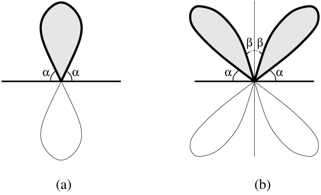
Figure 3: (a) One-petal solution, (b) two-petal solution. The mirror images in the lower half-plane is also shown.

Figure 4: One-petal solutions: $\alpha=\frac{\pi}{8}$ (dashed line), $\alpha=\frac{\pi}{4}$ (dotted line) and $\alpha=\frac{3\pi}{8}$ (solid line).

One-petal solution via integral equation.

The same results can be obtained in a different way, using an integral equation for the conformal map $f(w)$ which follows from the properties of the $M$-function. The function $M_{+}$ for the one-petal solution has only one cut which is the whole real axis and by virtue of (22) the jump across the cut must be a linear function. The coefficient can be fixed by analyzing the local behavior around the origin. Indeed, let $e^{i\theta(z)}=dz/|dz|$ be the unit tangent vector to the curve (represented as complex number) at a point $z$, then, by definition of the Schwarz function, $S^{\prime}(z)=e^{-2i\theta(z)}$ for $z$ on the curve in the upper half plane and $\bar{S}^{\prime}(z)=e^{-2i\theta(z)}$ for $z$ on the curve in the lower half plane. These formulas allow us to calculate discontinuity of the function $M^{\prime}$ (which obviously equals the discontinuity of $M^{\prime}_{+}$) across the real axis. Using (9) we find:

$$[M^{\prime}]:=M^{\prime}_{up}-M^{\prime}_{down}=\frac{1}{i}(2-S^{\prime}_{up}-\bar{S}^{\prime}_{down})=\frac{1}{i}(2-e^{-2i\alpha}-e^{2i\alpha})=-4i\sin^{2}\alpha$$ (29)

Thus in the upper half-plane

$$M_{+}=-2i\sin^{2}\alpha z+A,$$ (30)

and in the lower one

$$M_{+}=2i\sin^{2}\alpha z+A,$$ (31)

Using (7) we can express the sum of the values of $f(w)$ on the opposite sides of the cut from $-1$ to $1$ in the $w$-plane. Set $\{f(w)\}=f(w+i0)+f(w-i0)$, then

$$\{f(w)\}=2f(1/w)+i[M_{+}(f(1/w))]=(2-4\sin^{2}\alpha)f(1/w)=2\cos 2\alpha\,f(1/w)$$

where it is taken into account that

$$[M_{+}(f(w))]=M_{+}(f(w+i0))-M_{+}(f(w-i0))=-4i\sin^{2}\alpha f(w).$$

We have obtained the equation

$$\{f(w)\}=2\cos 2\alpha\,f(1/w),\quad\quad w\in[-1,\,1]$$ (32)

which determines the conformal map.

It can be transformed to an integral equation by means of the substitution

$$g(w)=\frac{f(w)}{\sqrt{w^{2}-1}}$$

which allows one to transform the mean value of the function $f$ on the cut to the jump of the function $g$. Note that the branch of the square root should be chosen such that $\sqrt{w^{2}\!-\!1}=w\sqrt{1\!-\!w^{-2}}$ be an odd function outside the unit circle. The symmetry of the petal implies that $f(-w)=-f(w)$, thus $g(-w)=g(w)$. In terms of the function $g$ equation (32) acquires the form

$$[g(w)]=-2i\cos 2\alpha\,\frac{g(1/w)}{w},\quad\quad w\in[-1,\,1]$$ (33)

The function $g$ is analytic everywhere in the $w$-plane except for the two branch points at $w=\pm 1$, with the jump across the cut $[-1,1]$ being given by (33). Taking into account that $g(\infty)=1$, we can represent it by an integral of the Cauchy type along the cut:

$$g(w)=1-\frac{2i\cos 2\alpha}{2\pi i}\int^{1}_{-1}\frac{g(1/x)dx}{x(x-w)}$$

Finally, using the fact that $g$ is an even function, we arrive at the integral equation

$$g(w)=1-\frac{2\cos 2\alpha}{\pi}\int^{1}_{0}\frac{g(1/x)dx}{x^{2}-w^{2}}$$ (34)

We know that $f(w)\propto(w-1)^{\frac{2\alpha}{\pi}}$ in a vicinity of $w=1$, so we need a solution such that $g(w)\propto(w-1)^{\frac{2\alpha}{\pi}-\frac{1}{2}}$ near $w=1$, and similarly for a vicinity of $w=-1$. Note that the exponent is the same $\gamma$ as in (25). Consider first the case of positive $\gamma$. After a further substitution $g(w)=(1-w^{-2})^{\gamma}G(w^{-2}),$ using the fact that $g(\pm 1)=0$ (valid for positive $\gamma$), we arrive at the equation

$$(1-x)^{\gamma-1}G(x)=\frac{\sin\pi\gamma}{\pi}\int^{1}_{0}\frac{t^{-1/2}(1-t)^{\gamma-1}G(t)dt}{1-xt}.$$ (35)

Comparing it with equation (42) from [9], we can immediately write down the solution:

$$G(t)=\,_{2}F_{1}\left(\begin{array}[]{c}\gamma,\gamma-1/2\\ {1/2}\end{array};t\right),$$

which is the same function as in (26). The map $f(w)$ is then given by the explicit formula (27). A direct substitution shows that the function $g(w)=f(w)/\sqrt{w^{2}-1}$ obeys the integral equation (34) for both positive and negative $\gamma$, $|\gamma|<1/2$.

Two-petal solution.

Consider now a two-petal pattern growing in the upper half-plane and symmetric w.r.t. the imaginary axis (Fig. 3). Let the angle between the two petals be $2\beta$. Clearly, the angles satisfy the condition $0<\beta<\pi/2-\alpha$. Now $V(w)$ has $4$ double poles. Two of them are at $w=\pm 1$. The symmetry implies that the other two poles are at $w=\pm i$. The function $V(w)$ is again uniquely determined by the conditions a), b), c):

$$V(w)=\frac{16\alpha}{\pi}\left(1-\frac{\alpha}{\pi}\right)\frac{w^{2}}{(w^{2}-1)^{2}}-\frac{8\beta}{\pi}\left(1-\frac{2\beta}{\pi}\right)\frac{w^{2}}{(w^{2}+1)^{2}}$$ (36)

Note that the same function corresponds to the angle $\pi/2-\beta$. The same substitution as above, $w=e^{x}$, $f(w)=(\mbox{sinh}\,x)^{1/2}\psi(x)$, brings equation (19) to the form

$$\psi^{\prime\prime}+\frac{\gamma(1-\gamma)}{\mbox{sinh}^{2}x}\,\psi-\frac{\delta(1-\delta)}{\mbox{cosh}^{2}x}\,\psi=\frac{1}{4}\,\psi$$ (37)

where $\gamma$ is as in (25) and $\delta=2\beta/\pi$. A further change of variables,

$$\psi=2(\mbox{sinh}\,x)^{\gamma}(\mbox{cosh}\,x)^{\frac{1}{2}-\gamma}F(1/\mbox{cosh}^{2}x)\,,\quad t=\frac{1}{\mbox{cosh}^{2}x}$$

puts the equation in the canonical hypergeometric form

$$t(1-t)F_{tt}+\left(\frac{1}{2}-(1+\gamma)t\right)F_{t}-\frac{1}{16}\Bigl{(}(2\gamma\!+\!2\delta\!-\!1)(2\gamma\!-\!2\delta\!+\!1)\Bigr{)}F=0.$$ (38)

Two linear independent solutions are

$$F^{(1)}(t)=\,_{2}F_{1}\left(\begin{array}[]{l}(2\gamma\!+\!2\delta\!-\!1)/4,\,(2\gamma\!-\!2\delta\!+\!1)/4\\ \\ \phantom{aaaaaa}1/2\end{array};\,t\right)$$

and

$$F^{(2)}(t)=\,t^{1/2}\,_{2}F_{1}\left(\begin{array}[]{l}(2\gamma\!+\!2\delta\!+\!1)/4,\,(2\gamma\!-\!2\delta\!+\!3)/4\\ \\ \phantom{aaaaaa}3/2\end{array};\,t\right)$$

For the function $\psi$ the first solution gives

$$\psi(x)=(\mbox{sinh}\,x)^{\gamma}(\mbox{cosh}\,x)^{\frac{1}{2}-\gamma}\,_{2}F_{1}\left(\begin{array}[]{l}(2\gamma\!+\!2\delta\!-\!1)/4,\,(2\gamma\!-\!2\delta\!+\!1)/4\\ \\ \phantom{aaaaaa}1/2\end{array};\,\mbox{cosh}^{-2}x\right)$$

Passing to the function $f(w)$ and to the original angles $\alpha$, $\beta$, we have:

$$f(w)=w(1-w^{-2})^{\frac{2\alpha}{\pi}}(1+w^{-2})^{1-\frac{2\alpha}{\pi}}\,_{2}F_{1}\left(\begin{array}[]{l}\displaystyle{\frac{\alpha\!+\!\beta}{\pi}-1/2,\,\,\frac{\alpha\!-\!\beta}{\pi}}\\ \\ \phantom{aaaaa}1/2\end{array};\,\frac{4}{(w+w^{-1})^{2}}\right)$$ (39)

The symmetry implies that the conformal map must be an odd function of $w$. The function given by (39) is indeed odd while the second solution, $F^{(2)}$, leads to an even function of $w$. Using the argument principle, one can see that for $0<\beta<\alpha<\pi/2$ the derivative $f^{\prime}(w)$ has no zeros in the exterior of the unit circle. Therefore, $f(w)$ given by (39) is the conformal map for the two-petal solution.

Note that this function looks somewhat simpler in the variable $p=w+w^{-1}$ living in the upper half plane:

$$z(p)=p(1-4p^{-2})^{\alpha/\pi}\,_{2}F_{1}\left(\begin{array}[]{l}\displaystyle{\frac{\alpha\!+\!\beta}{\pi}-1/2,\,\,\frac{\alpha\!-\!\beta}{\pi}}\\ \\ \phantom{aaaaa}1/2\end{array};\,4p^{-2}\right)$$ (40)

The analytic continuation of the function (40) to the region $|p|<2$ reads:

$$\begin{array}[]{r}\displaystyle{z(p)=2(1\!-\!p^{2}/4)^{\alpha/\pi}\left[ie^{-i\beta}\frac{\Gamma(\frac{1}{2})\Gamma(\frac{1}{2}-\frac{2\beta}{\pi})}{\Gamma(\frac{\alpha-\beta}{\pi})\Gamma(1\!-\!\frac{\alpha+\beta}{\pi})}\left(\frac{p}{2}\right)^{2\beta/\pi}\!\!_{2}F_{1}\left(\begin{array}[]{l}\frac{\alpha\!+\!\beta}{\pi}\!-\!\frac{1}{2},\,\,\frac{\alpha\!+\!\beta}{\pi}\\ \\ \phantom{aa}\frac{2\beta}{\pi}\!+\!\frac{1}{2}\end{array};\,\frac{p^{2}}{4}\right)\right.}\\ \\ \displaystyle{\left.+\,e^{i\beta}\frac{\Gamma(\frac{1}{2})\Gamma(\frac{2\beta}{\pi}-\frac{1}{2})}{\Gamma(\frac{\alpha+\beta}{\pi}-\frac{1}{2})\Gamma(\frac{1}{2}\!-\!\frac{\alpha-\beta}{\pi})}\left(\frac{p}{2}\right)^{1-2\beta/\pi}\!\!_{2}F_{1}\left(\begin{array}[]{l}\frac{\alpha\!-\!\beta}{\pi}\!+\!\frac{1}{2},\,\,\frac{\alpha\!-\!\beta}{\pi}\\ \\ \phantom{aa}\frac{3}{2}\!-\!\frac{2\beta}{\pi}\end{array};\,\frac{p^{2}}{4}\right)\right]\phantom{aa}}\end{array}$$ (41)

The boundary of the two-petal pattern in the upper half plane is obtained as $z(p+i0)$ for $-2<p<2$.

In the case $\beta=\alpha$ the hypergeometric function in (40) becomes trivial (equal to $1$). The corresponding conformal map appears to be a map to a slit domain: the function $z(p)=p(1-4p^{-2})^{\alpha/\pi}$ takes the upper half plane to the upper half plane cut along two straight segments emanating from $0$ to the NE and NW quadrants at the angle $\alpha$ to the real axis. In fact this means that $\beta=\pi/2-\alpha$ rather than $\alpha$ but as it was already mentioned, the function (36) is the same in both cases.

(a) $\alpha=\frac{\pi}{8},~{}\beta=\frac{\pi}{16}$

(b) $\alpha=\frac{\pi}{8},~{}\beta=\frac{\pi}{8}$

(c) $\alpha=\frac{\pi}{4},~{}\beta=\frac{\pi}{16}$

(d) $\alpha=\frac{5\pi}{16},~{}\beta=\frac{\pi}{16}$

Figure 5: Two-petal solutions

Some typical two-petal solutions are shown in Fig. 5. The following cases are to be distinguished:

• $\alpha\in(0,\frac{\pi}{4})$

  • $\beta\in(0,\alpha)$ – the petals are shown in Fig. 5 (a), they become very thin as $\beta$ approaches $\alpha$ from below,

  • $\beta=\alpha$ – the petals degenerate to segments (Fig. 5 (b)),

  • $\beta\in(\alpha,\frac{\pi}{2}-\alpha)$ – the solution does not exist because the map is not conformal;

• $\alpha=\frac{\pi}{4}$, $\beta\in(0,\frac{\pi}{4})$ – the function $f(w)$ can be expressed through elementary functions:

  $$f(w)=\left(w+w^{-1}\right)\left(1-\frac{4}{\left(w+w^{-1}\right)^{2}}\right)^{1/4}\cos\left[2\left(\frac{1}{4}-\frac{\beta}{\pi}\right)\arcsin\left[\frac{2}{w+w^{-1}}\right]\right],$$ (42)

  a typical pattern is shown in (Fig. 5 (c)), the solution degenerates at $\beta=\frac{\pi}{4}$.

• $\alpha\in(\frac{\pi}{4},\frac{\pi}{2})$

  • $\beta\in(\alpha,\frac{\pi}{2})$ – the petals are shown in Fig. 5 (d),

  • $\beta=\frac{\pi}{2}-\alpha$ – the petals degenerate to segments,

  • $\beta\in(\frac{\pi}{2}-\alpha,\alpha)$ – the solution does not exist because the map is not conformal.

Let us also note that the shape of two-petal solutions at small $\beta$ becomes close to one-petal solutions with the same $\alpha$ (Fig. 6), as it could be expected from the differential equations.

Figure 6: One-petal solution at $\alpha=\frac{\pi}{4}$ and two-petal solution at $\alpha=\frac{\pi}{4}$ and $\beta=\frac{\pi}{50}$.

References

- [1] A. Zabrodin, Growth of fat slits and dispersionless KP hierarchy, J. Phys. A: Math. Theor. 42 (2009) 085206 (23pp).
- [2] S. D. Howison, Complex variable methods in Hele-Shaw moving boundary problems, Euro. J. Appl. Math. 3 (1992) 209-224.
- [3] P. J. Davis, The Schwarz function and its applications, The Carus Math. Monographs, No. 17, The Math. Assotiation of America, Buffalo, N.Y., 1974.
- [4] H.Thome, M.Rabaud, V.Hakim and Y.Couder, The Saffman-Taylor instability: From the linear to the circular geometry, Phys. Fluids A1 (1989) 224-240
- [5] M.Ben Amar, Exact self-similar shapes in viscous fingering, Phys. Rev. A43 (1991) 5724-5727; Viscous fingering in a wedge, Phys. Rev. A44 (1991) 3673-3685
- [6] Y. Tu, Saffman-Taylor problem in sector geometry: Solution and selection, Phys. Rev. A44 (1991) 1203-1210.
- [7] R.Combescot, Saffman-Taylor fingers in the sector geometry, Phys. Rev. A45 (1992) 873-884
- [8] I.Markina and A.Vasil’ev, Scientia 9 (2003) 33-43; Euro. J. Appl. Math. 15 (2004) 781-789.
- [9] Ar. Abanov, M. Mineev-Weinstein and A. Zabrodin, Self-similarity in Laplacian growth, Physica D 235 (2007) 62-71.
- [10] A.I.Markushevich, Theory of analytic functions. vol. 2, Moscow, Nauka, 1968.