Parametrization of the transfer matrix: for one-dimensional Anderson model with diagonal disorder

Abstract

In this paper, we developed a new parametrization method to calculate the localization length in one-dimensional Anderson model with diagonal disorder. This method can avoid the divergence difficulty encountered in the conventional methods and significantly save computing time as well.

I Introduction

The tight-binding Anderson model Anderson (1958) is a standard model for disordered systems. It predicted that with random on-site energies whose strength of disorder is above a critical value, the electrons are localized in a certain spatial region. The transition from metal to insulator by increasing the strength of disorder is called Anderson transition. According to the single-parameter scaling theory Abrahams et al. (1979), there is no metallic regime in the disordered system with dimension $d\leq 2$ Markos (2006); Evers and Mirlin (2008). With long-range correlated disorder, even in one-dimensional systems, there can exist extended electronic states and a true Anderson transition with mobility edges was observed De Moura and Lyra (1998).

One-dimensional systems are the simplest case to study. There were a number of review articles on the problem of localization in one-dimensional systems Ishii (1973); Abrikosov and Ryzhkin (1978); Erdos and Herndon (1982); Gogolin (1982). Recently, articles about the general analytical methods Rodriguez (2006), anomalous behaviors at band center Deych et al. (2003); Schomerus and Titov (2003), ensemble-averaged conductance fluctuations Hilke (2008), and discrete Anderson nonlinear Schrödinger equations Garcia-Mata and Shepelyansky (2009) were appeared in the major journals, indicating the topic is still a hot one.

One of the important one and quasi-one dimensional real systems is the DNA molecules. The topics of charge transport in DNA and the feasibility of constructing DNA-based devices, have kindled a heated debate within the scientific community Porath et al. (2005). Various theoretical models about charge transport in DNA were generalized from the original one-dimensional tight-binding model of Anderson Anderson (1958)

$$H=\sum_{i}\epsilon_{i}c^{\dagger}_{i}c_{i}+\sum_{j\neq i}t_{ji}c^{\dagger}_{j}c_{i},$$ (1)

where $\epsilon_{i}$ is the $i$th on-site energy given by a random distribution, and $t_{ji}$ is the hopping energy from the $i$th site to the $j$th site. The one-dimensional Anderson model with diagonal disorder (all $t_{ji}$ equal to $t$) expressed in terms of the Schrödinger equation is

$$\psi_{i-1}+\psi_{i+1}=(E-\epsilon_{i})\psi_{i},$$ (2)

where $\psi_{i}$ is the wave function on the $i$th site, $E$ is the eigenenergy. The hopping energy $t$ has been set as energy unit. Generalizations to more realistic models of DNA molecules take into account of correlations, random hopping energies, coupled multichains, and so on Bagci and Krokhin (2007); Guo and Xu (2007); Liu et al. (2007); Rodriguez (2006); Xiong and Wang (2005); Ndawana et al. (2004); Zhang and Ulloa (2004); Heinrichs (2002); Eilmes et al. (1998).

Of the many approaches which have been developed for numerical simulations of disordered systems, the transfer matrix method has proved the most productive MacKinnon (2003); Pendry (1994). Introducing a two component vector $\Psi_{i}=(\psi_{i}\;\;\psi_{i-1})^{t}$, Eq. (2) can be written as

$$\Psi_{i+1}=\left(\begin{array}[]{c}\psi_{i+1}\\ \psi_{i}\end{array}\right)=\left(\begin{array}[]{cc}E-\epsilon_{i}&-1\\ 1&0\end{array}\right)\left(\begin{array}[]{c}\psi_{i}\\ \psi_{i-1}\end{array}\right)=\mathbf{T}_{i}\Psi_{i},$$ (3)

where $\mathbf{T}_{i}$ is the so-called transfer matrix. Here only the diagonal disorder is considered, in which case the transfer matrix is symplectic. With transfer matrix we can get the wavefunction $\psi_{L}$ on site-$L$ propagating from site-1 with wavefunction $\psi_{1}$ for arbitrary $L$ in principle by $\Psi_{L}=\mathbf{T}_{L}\mathbf{T}_{L-1}\cdots\mathbf{T}_{1}\Psi_{1}$.

Traditional transfer matrix method has to calculate detailed physical properties for a long chain, then to use scaling technique to reveal the properties under the thermodynamic limit; and it requires a stabilization procedure to overcome the overflow problem, typically about every twelve iteration MacKinnon (2003). In this paper we propose a parametrization method to deal with the transfer matrix of one-dimensional Anderson model with uncorrelated diagonal disorder. With this method, we directly calculate in the localization regime under the thermodynamic limit; and it is easy to calculate the localization length for arbitrary strength of disorder. Particularly, it is easier to calculate moderate disorder than both weak and strong disorder, in which cases it needs more numerical techniques to obtain the results in our method.

II Parametrization of the transfer matrix

The transfer matrix $\mathbf{T}_{i}$ in Eq. (3) is a symplectic matrix, which satisfies the condition $\mathbf{A}^{t}\mathbf{\Omega}\mathbf{A}=\mathbf{\Omega}$, where $\mathbf{A}^{t}$ is the transpose of a $2n\times 2n$ matrix $\mathbf{A}$, and $\mathbf{\Omega}$ is a fixed nonsingular, skew-symmetric matrix. Typically $\mathbf{\Omega}$ is chosen to be a block matrix

$$\mathbf{\Omega}=\left[\begin{array}[]{cc}\mathbbold{0}&\mathbbold{1}\\ -\mathbbold{1}&\mathbbold{0}\end{array}\right],$$ (4)

where $\mathbbold{0}$ and $\mathbbold{1}$ are $n\times n$ zero matrix and unit matrix respectively. It is easily shown from the definition that the transpose of a symplectic matrix is also a symplectic matrix.

Let $\mathbf{M}_{L}=\mathbf{T}_{1}\mathbf{T}_{2}\cdots\mathbf{T}_{L}$ and $v_{i}=E-\epsilon_{i}$. Since the symplectic matrices form a group, the product of $\mathbf{M}^{t}_{L}$ and $\mathbf{M}_{L}$ is symplectic and real symmetric. Thus, it can be diagonalized by an orthogonal matrix $\mathbf{U}(\theta_{L})$,

$$\mathbf{U}(\theta_{L})\mathbf{M}^{t}_{L}\mathbf{M}_{L}\mathbf{U}(-\theta_{L})=\left(\begin{array}[]{cc}e^{\lambda_{L}}&\\ &e^{-\lambda_{L}}\end{array}\right),$$ (5)

where

$$\mathbf{U}(\theta_{L})=\left(\begin{array}[]{cc}\cos\theta_{L}&-\sin\theta_{L}\\ \sin\theta_{L}&\cos\theta_{L}\end{array}\right).$$ (6)

The $2\times 2$ symplectic matrix has a property that the two eigenvalues are reciprocal to each other. Hence, $\mathbf{M}^{t}_{L}\mathbf{M}_{L}$ can be expressed in terms of $\lambda_{L}$ and $\theta_{L}$,

$$\mathbf{M}^{t}_{L}\mathbf{M}_{L}=\cosh\lambda_{L}\mathbbold{1}+\sinh\lambda_{L}\left(\begin{array}[]{cc}\cos 2\theta_{L}&-\sin 2\theta_{L}\\ -\sin 2\theta_{L}&-\cos 2\theta_{L}\end{array}\right),$$ (7)

here $\mathbbold{1}$ is a $2\times 2$ unit matrix and the two parameters $\lambda_{L}$ and $\theta_{L}$ play important roles to parameterize the transfer matrices.

Making use of the definition of $\mathbf{M}_{L}$,

$$\mathbf{M}^{t}_{L+1}\mathbf{M}_{L+1}=\left(\begin{array}[]{cc}v_{L+1}&1\\ -1&0\end{array}\right)\mathbf{M}^{t}_{L}\mathbf{M}_{L}\left(\begin{array}[]{cc}v_{L+1}&-1\\ 1&0\end{array}\right),$$ (8)

and substituting the expression for $\mathbf{M}^{t}_{L}\mathbf{M}_{L}$ in Eq. (7), we can easily obtain the recursion relations for $\lambda$ and $\theta$,

$$\cosh\lambda_{L+1}=(1+\frac{v_{L+1}^{2}}{2})\cosh\lambda_{L}+(\frac{v_{L+1}^{2}}{2}\cos 2\theta_{L}-v_{L+1}\sin 2\theta_{L})\sinh\lambda_{L}$$ (9)

$$\sinh\lambda_{L+1}\cos 2\theta_{L+1}=[(\frac{v_{L+1}^{2}}{2}-1)\cos 2\theta_{L}-v_{L+1}\sin 2\theta_{L}]\sinh\lambda_{L}+\frac{v_{L+1}^{2}}{2}\cosh\lambda_{L}$$ (10)

$$\sinh\lambda_{L+1}\sin 2\theta_{L+1}=v_{L+1}\cosh\lambda_{L}+(v_{L+1}\cos 2\theta_{L}-\sin 2\theta_{L})\sinh\lambda_{L}.$$ (11)

In the localization regime, the localization length is finite. For sufficiently long chains (depending on the strength of localization), the exponent $\lambda$ of the eigenvalue will be approaching to infinity. Hence after dividing Eq. (11) by Eq. (10) and taking the limit $\lambda\rightarrow\infty$ or $\tanh\lambda_{L}\rightarrow 1$, we get the recursion relation of $2\theta$ in the localization regime,

$$\tan 2\theta_{L+1}=\frac{v_{L+1}(1+\cos 2\theta_{L})-\sin 2\theta_{L}}{v_{L+1}^{2}(1+\cos 2\theta_{L})/2-v_{L+1}\sin 2\theta_{L}-\cos 2\theta_{L}}.$$ (12)

Using the basic relations of trigonometric functions, it is easy to derive a much simpler recursion relation of $\theta$, Eq. (13), from Eq. (12),

$$\tan\theta_{L+1}=\frac{1}{v_{L+1}-\tan\theta_{L}}.$$ (13)

From Eq. (13) it is apparent that if $v_{L+1}=0$, $\theta_{L+1}=\theta_{L}\pm\pi/2$, which is also indicated in Eq. (12). Eq. (13) can also be written as a continued fraction

$$\tan\theta_{L}=\frac{1}{\displaystyle v_{L}-\frac{1}{\displaystyle v_{L-1}-\cdots-\frac{1}{\displaystyle v_{2}-\tan\theta_{1}}}}.$$ (14)

In this form we can see that, for each specified chain, $\theta_{L}$ is completely determined by the sequence of random on-site energies and the eigenenergy $E$ in the Schrödinger equation. We should bear in mind that all the results we have in this paper are in the localization regime under the thermodynamic limit. Therefore, although we label the first site as site 1, it does not mean that site 1 starts from the very beginning, there are sufficiently many sites before it. Furthermore, as an initial input, the effect of $\theta_{1}$ will vanish for sufficiently large $L$.

Now we derive the probability density of $\theta$ from the known random distribution of $\epsilon$ (or $v=E-\epsilon$). And we can calculate the localization length directly through the probability density of $\theta$. Define $t\equiv\tan\theta$. From Eq. (13), we have an integral equation for the probability density function of $t$

$$p_{c}(\frac{1}{t}) = \int_{-\infty}^{\infty}\int_{-\infty}^{\infty}p_{t}(t^{\prime})p_{v}(v)\delta[\frac{1}{t}-(v-t^{\prime})]\mathrm{d}t^{\prime}\mathrm{d}v$$ (15)

$$= \int_{-\infty}^{\infty}p_{t}(t^{\prime})p_{v}(\frac{1}{t}+t^{\prime})\mathrm{d}t^{\prime},$$

where $p_{t}(t)$, $p_{c}(\displaystyle\frac{1}{t})$, and $p_{v}(v)$ are the probability density functions for $\tan\theta$, $\cot\theta$, and $v$ respectively. With the relations of the probability density functions,

$$p(\theta)={1\over\cos^{2}\theta}p_{t}(t)={1\over\sin^{2}\theta}p_{c}(\frac{1}{t}),$$ (16)

the integral equation of the probability density function $p(\theta)$ becomes

$$p(\theta)=\frac{1}{\sin^{2}\theta}\int_{-\pi/2}^{\pi/2}p(\theta^{\prime})p_{v}(\frac{1}{\tan\theta}+\tan\theta^{\prime})\mathrm{d}\theta^{\prime}.$$ (17)

If we can obtain the solution of $p(\theta)$ from Eq. (17), the inverse localization length is given by Eq. (9)

$$\frac{1}{\xi} = \gamma=\frac{1}{2}\langle\lambda_{L+1}-\lambda_{L}\rangle$$ (18)

$$= \frac{1}{2}\int_{-\pi/2}^{\pi/2}\int_{-\infty}^{\infty}p(\theta)p_{v}(v)\ln(1+v^{2}\cos^{2}\theta-v\sin 2\theta)\mathrm{d}v\mathrm{d}\theta,$$

where $\gamma$ is the so-called Lyapunov exponent. The second line is obtained when $\lambda\rightarrow\infty$, hence $\cosh\lambda_{L+1}/\cosh\lambda_{L}\rightarrow\exp(\lambda_{L+1}-\lambda_{L})$ and $\tanh\lambda_{L}\rightarrow 1$. For uncorrelated disorder considered in this paper, $p(\theta)$ and $p_{v}(v)$ are independent of each other, thus the above equation is correct for sufficiently long chains in the localization regime. In Rodriguez (2006), a similar expression was obtained from a different starting point for $p_{v}(v)$ as a discrete distribution and the parameter $\theta$ was chosen to be real at the beginning.

It should be mentioned that from the original Schrödinger equation we have

$$z_{L+1}=\frac{1}{v_{L+1}-z_{L}},$$ (19)

where $z_{L}=\psi_{L}/\psi_{L+1}$. This is exactly the form of Eq. (13). The difference is that $z$ is a complex number while $\tan\theta$ is real. We found that for sufficiently large $L$ with the same random sequence, the real part of $z_{L}$ is the same as $\tan\theta_{L}$ and its imaginary part goes to zero in the localization regime. $z_{L}$ and $\tan\theta_{L}$ are essentially the same quantity when $L$ is sufficiently large in the localization regime. Thus the phase difference between $\psi_{L}$ and $\psi_{L+1}$ is 0 or $\pi$ and the ratio of their amplitudes is $\mathrm{Re}(\psi_{L}/\psi_{L+1})\rightarrow\tan\theta_{L}$ for sufficiently large $L$ in the localization regime. And the expression for the localization length of $z$ in Ishii (1973) can be rewritten in our symbols as the following,

$$\gamma(E)=-\int_{-\pi/2}^{\pi/2}\mathrm{d}\theta p(\theta)\ln\left|\tan\theta\right|,$$ (20)

once we solve the probability density $p(\theta)$ from Eq. (17), where the dependence on the eigenenergy $E$ is implicitly included in $p(\theta)$. The $z$ defined in Ishii (1973) is the inverse of ours, thus we have a minus sign in our equation. Eq. (18) and Eq. (20) are equivalent

$$\frac{1}{2}\iint p(\theta)p_{v}(v)\ln(1+v^{2}\cos^{2}\theta-v\sin 2\theta)\mathrm{d}v\mathrm{d}\theta$$

$$= \frac{1}{2}\left\{\int p(\theta)\ln\cos^{2}\theta\mathrm{d}\theta+\iiint\mathrm{d}\theta\mathrm{d}v\mathrm{d}\cot\theta^{\prime}p(\theta)p_{v}(v)\ln[1+(v-\tan\theta)^{2}]\delta[\cot\theta^{\prime}-(v-\tan\theta)]\right\}$$

$$= -\int p(\theta)\ln|\tan\theta|\mathrm{d}\theta.$$

However, Eq. (18) is more appropriate for numerical calculation because it requires less accurate $p(\theta)$ than Eq. (20).

From the above description, we can experience benefits of our method. We do not have to use the recursive relation Eq. (13) to calculate the sequence $\theta_{L}$, nor $\lambda_{L}$. Although the recursive relation is very simple, the time consumption of the computation of $\theta_{L}$ is still the same as in the conventional transfer matrix method within the same accuracy. Moreover, the conventional transfer matrix method has a problem that it has to care about the overflow problem especially for strong disorder. This is not a problem in our method. We can calculate arbitrary strength disorder. More importantly, we can easily calculate moderate strength disorder, which is difficult for analytical methods.

III Numerical technique

Eq. (17) shall be solved numerically in a discrete matrix form by using self-consistent iterative procedure. In principle, we can get the probability density $p(\theta)$ for any known random distribution $p_{v}(v)$. In this paper we only considered two distributions: Lorentzian and Gaussian. For the Lorentzian distribution, there are exact analytical results Ishii (1973) and for the Gaussian distribution, there are analytical results in the weak and strong disorder limits Izrailev et al. (1998). We will compare our numerical results with theirs.

From the r.h.s of Eq. (17), we can see that there is a removable singularity at $\theta=0$ in both of the Lorentzian and Gaussian distributions in the numerical computation. Thus we need to use interpolation to obtain $p(\theta)$ near $\theta=0$. For the Lorentzian distribution we use six-points interpolation and for the Gaussian distribution we use seven-points interpolation with a condition $p(0)=[p(\pi/2)+p(-\pi/2)]/2$. This condition can be easily derived from Eq. (15). Let $t^{\prime\prime}=t^{\prime}+\displaystyle{\frac{1}{t}}$, then Eq. (15) becomes,

$$p_{c}(\frac{1}{t})=\int_{-\infty}^{\infty}p_{t}(t^{\prime\prime}-\frac{1}{t})p_{v}(t^{\prime\prime})\mathrm{d}t^{\prime\prime}.$$ (21)

For $|t^{\prime\prime}|\ll|1/t|$, $p_{t}(t^{\prime\prime}-1/t)\approx p_{t}(-1/t)$, so Eq. (21) can become approximately,

$$p_{c}(\frac{1}{t})\approx p_{t}(-\frac{1}{t})\int_{-\infty}^{\infty}p_{v}(t^{\prime\prime})\mathrm{d}t^{\prime\prime},$$ (22)

and we have $\displaystyle\lim_{t\rightarrow 0^{\pm}}p_{c}(\frac{1}{t})=\lim_{t\rightarrow 0^{\pm}}p_{t}(-\frac{1}{t})$. This relation can be rewritten in terms of the probability density of $\theta$ as $p(\theta\rightarrow 0^{\pm})=p(\mp\pi/2)$ by using Eq. (16). We should emphasize that for the Lorentzian distribution this relation is not valid. The range of $\theta$ need to use interpolation is determined by $|\theta|<\sqrt{m\pi/N\sigma}$, where $m$ is a number we choose to ensure that the profile of $p(\theta)$ near $\theta=0$ is smooth (we assume this is true for nonsingular distributions $p_{v}(v)$), $N$ is the number of equally spaced abscissas points where the integrands are evaluated and $\sigma$ is the parameter of the distributions, $p_{v}(v)=\displaystyle\frac{1}{\sigma\sqrt{\pi}}\exp[-(v-E)^{2}/\sigma^{2}]$ and $p_{v}(v)=\displaystyle\frac{1}{\pi}\frac{\sigma}{\sigma^{2}+(v-E)^{2}}$, respectively. The magnitude of $\sigma$ in the distribution function represents the strength of disorder. With $p(\theta)$ in the hand, we can use Eq. (18) to calculate the localization length numerically for cases of uncorrelated disorder.

In our method, errors come from the value $N$ we choose as the number of discrete components of $p(\theta)$ and where the cut-off is in the infinite range of the integration with respect to $v$. Basically, large $E$ or small $\sigma$ need large $N$, and large $\sigma$ needs a large range of integration and a correction to remedy the effect of finite integration range. When $N$ is large, it spends a long time on the computation of $p(\theta)$. In fact, this is always the main part of the computation time no matter how large $N$ is. When the range of integration for $v$ is large, more CPU time is consumed to compute the integration of $v$; increasing $N$ does not improve the result when the range of integration remain unchanged; the result is sensitive to the range of integration of $v$ for the Gaussian distribution, while for the Lorentzian distribution it is not. The reason should be that the Gaussian distribution varies more dramatically than the Lorentzian distribution.

IV Results and discussions

As mentioned in the previous section, we obtained $p(\theta)$ numerically from Eq. (17) first. We performed the integral with respect to $v$ by using Romberg’s method, and solved the integral equation by using a discrete matrix form, where $p(\theta)$ was written in a vector form with $N$ components. Figure 1 shows the solutions of $p(\theta)$ for the Lorentzian and Gaussian distributions respectively. When $E=0$, $p(\theta)$ is symmetric respected to $\theta=0$. As $E$ becomes large, $p(\theta)$ becomes a Dirac $\delta$-function. The position of the peak does not change monotonically with the increase of $E$. The salient difference of $p(\theta)$ between the two distributions is, when $E$ is small, the Lorentzian distribution has only one peak, while the Gaussian distribution has two.

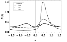
Figure 1: Probability density $p(\theta)$ obtained numerically from Eq. (17) with $E$ = 0 (solid), 1 (dashed), 2 (dotted) when $\sigma=1$ for (a) the Lorentzian distribution $p_{v}(v)=\displaystyle\frac{1}{\pi}\frac{1}{1+(v-E)^{2}}$, (b) the Gaussian distribution $p_{v}(v)=\displaystyle\frac{1}{\sqrt{\pi}}\exp[-(v-E)^{2}]$.

After we had the probability density $p(\theta)$, the inverse localization length $\gamma$ was calculated from Eq. (18) numerically. For the Lorentzian distribution, the analytical results were already available in Ishii (1973),

$$\gamma(E,\sigma)=\mathrm{arccosh}\frac{\sqrt{(2+E)^{2}+\sigma^{2}}+\sqrt{(2-E)^{2}+\sigma^{2}}}{4}.$$ (23)

Our numerical results for the Lorentzian distribution are shown in Figure 2, where we plot $\gamma$ versus $E$ with $\sigma=0.1,~{}1,~{}10$ respectively with the comparison between our results and the analytical results. We found that they all coincide in excellence, and we can not see the difference from the figure. We used the Romberg integration method to perform a numerical integral with respect to $v$, and we made a cut-off to the infinity range of integration, so the real range is finite from $E-10^{3}\sigma$ to $E+10^{3}\sigma$. Because the Lorentzian distribution does not decay rapidly to zero when $\sigma$ was large, we need to consider the compensation of the contribution from the cut-out range. In fact, the integral of the cut-out range can be approximately integrated analytically, and the correction was $4\ln|10^{3}\sigma\cos\theta|/10^{3}\pi$. This correction would eliminate a constant difference between the numerical result and the analytical result. For weak disorder $\sigma=0.1$ shown in Figure 2, with increasing $E$, the number of mesh points $N$ should go from 2000 to 9000 in order to obtain the right result, otherwise the result $\gamma$ will be much smaller than the analytical result. For strong disorder $\sigma=10$ shown in Figure 2, the number of mesh points $N=2000$ with the correction is good enough to reach the desired accuracy, no matter how large $E$ is.

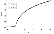
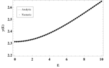
Figure 2: Comparison between the analytical and our numerical results for the Lorentzian distribution with $\sigma$ = (a) 0.1, (b) 1, and (c) 10, respectively.

Numerical calculation of Eq. (20) and Eq. (18) gave the same result in Figure 3. This is one evidence of the conclusion that $z$ and $\tan\theta$ are the same quantity when the chain is long enough in the localization regime.

Figure 3: Inverse of the localization length $\gamma(E)$ obtained from Eq. (20) and Eq. (18) for the Gaussian (solid) and the Lorentzian (dashed) distributions.

From Figure 3, it can be seen that when in the band $E=0$ to 2, the difference of $\gamma$ between the Lorentzian and the Gaussian distributions is nearly a constant. It seems that they have the same behavior in the band. When $E$ becomes large, the $\gamma$ of the two distributions increase and go to the same value. The reason is that when $E\rightarrow\infty$, both the Lorentzian and Gaussian distributions become a $\delta$-function. For example, for the Lorentzian distribution, let $y=v/E-1$,

$$\lim_{E\rightarrow\infty}\frac{1}{\pi}\frac{\sigma}{(v-E)^{2}+\sigma^{2}}\mathrm{d}v=\delta(y)\mathrm{d}y,$$ (24)

then

$$\int_{-\infty}^{\infty}f(v)p_{v}(v)\mathrm{d}v = \int_{-\infty}^{\infty}f(Ey+E)\delta(y)\mathrm{d}y$$ (25)

$$= f(E).$$

Thus if $p(\theta)$ at large $E$ are the same for different $p_{v}(v)$, $\gamma(E)$ will be the same. We have checked that this is true for the two distributions.

In Figure 4 we plot $\gamma$ versus $\sigma$. For the Lorentzian distribution, the results also coincide well with Eq. (23). And we found that all the five lines can be fitted well by $\gamma(\sigma)=a+b\sqrt{\sigma}+c\sigma+d\sigma^{2}$. For all the five lines, $d$ is always at least one order smaller than $b$ and $c$. For the Gaussian distribution, this is also true when $E$ is in the band. When $E>2$ out of the band, the behavior of the Gaussian distribution is very different and it can not be fitted by the above formula. When $\sigma$ becomes large, $\gamma(\sigma)$ becomes the same for different $E$. This is apparent in Figure 4 for the Lorentzian distribution. Similar to the derivation of large $E$, when $\sigma$ grows large, the difference between $p_{v}(v)$ with different $E$ vanishes. And this can be understood that when the width of the distribution becomes large, the position of the peak is irrelevant.

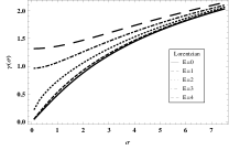
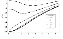
Figure 4: Inverse of the localization length $\gamma(\sigma)$ from Eq. (18) for (a) the Lorentzian distribution and (b) the Gaussian distribution with $E=0,1,2,3,4$ (from bottom to top).

In Izrailev et al. (1998) the authors provided analytical results for the Gaussian distribution with weak and strong disorder, which are summarized as follows,

$$\gamma(E,\sigma)=\left\{\begin{array}[]{r@{\quad,\quad}l}W^{2}/105.045\cdots&E=0\\ W^{2}/24(4-E^{2})&0<E<2\\ 0.289\cdots(\delta^{2})^{1/3}&E=2\end{array}\right..$$ (26)

In Izrailev et al. (1998), the strength of disorder are represented by parameters $W$ or $\delta$, which can be expressed in terms of $\sigma$ in our paper by $W^{2}=6\sigma^{2}$ and $\delta^{2}=\sigma^{2}/2$.

For the purpose of comparison, we showed the fitting formulae of our numerical data at weak disorder $0<\sigma<1$ in Table 1.

$E$	Lorentzian	Gaussian
0	$0.49\sigma$	$0.056\sigma^{2}$
1	$0.55\sigma$	$0.081\sigma^{2}$
2	$0.72\sqrt{\sigma}$	$0.24\sigma^{2/3}$
3	$0.96+0.11\sigma^{2}$	$0.96-0.063\sigma^{2}$
4	$1.32+0.045\sigma^{2}$	$1.32-0.022\sigma^{2}$

Table 1: Fit for weak disorder $0<\sigma<1$

The ratio of the coefficients of $E=1$ and $E=0$ derived from Eq. (26) is approximately 1.46 and the ratio of our numerical results calculated from Table 1 is approximately 1.45. At the band edge $E=2$, our result is $\gamma(2)\approx 0.24\sigma^{2/3}$, i.e. approximately $0.30\delta^{2/3}$. Therefore, our results confirmed the anomalous behavior of weak disorder at the band center $E=0$ Kappus and Wegner (1981); Derrida and Gardner (1984); Czycholl et al. (1981) and the band edge $E=2$ Derrida and Gardner (1984). Furthermore, our numerical result gave an expression for strong disorder at $E=1$, $\gamma(\sigma)=-0.80+1.00\ln\sigma$, which is in excellent agreement with the result of Izrailev et al. (1998), where $\gamma(\sigma)=-0.797\cdots+\ln\sigma$ when $E$ is in the band.

We noticed that for the Lorentzian distribution, the results can be obtained from the exact expression Eq. (23) for small and large $\sigma$ limits respectively. For strong disorder, $\gamma(\sigma)=\ln\sigma$ and our fitting formulae is $\gamma(\sigma)=1.00\ln\sigma$. It seems that the Lorentzian distribution should not have the anomalous behavior at the band center or band edge. However, it is apparent from Table 1 that at $E=2$, the Lorentzian distribution also has an anomalous behavior similar to that of the Gaussian distribution. On the other hand, it should be mentioned that $E=0$ may should be seen as a boundary of two bands rather than the center of one band Deych et al. (2003). As shown in Figure 1, the Lorentzian distribution has only one peak, while the Gaussian distribution has two when $E$ is small.

V Conclusions

In this paper, we derived a parametrization method to deal with the transfer matrix of the one-dimensional Anderson model with diagonal uncorrelated disorder. With this method, we directly calculated the localization length under the thermodynamic limit in the localization regime. It avoids the difficulties faced by the traditional transfer matrix method; and without the sampling process, the accuracy can be improved easily. As we showed, the results of our method coincide very well with the known analytical results of the Lorentzian and the Gaussian distributions, including the anomalous behaviors at the band center and the band edge. It is quite efficient when the distribution of diagonal disorder is nonsingular, especially for moderate disorder. Furthermore, we found that the Lorentzian distribution should give clues to the anomalies in the Gaussian distribution. Although it faces some difficulties for the cases like off-diagonal disorder or correlated disorder, this method can be generalized to the coupled multichain system with diagonal uncorrelated disorder.