Phase Shift in the Whitham Zone for the Gurevich-Pitaevskii Special Solution of the Korteweg-de Vries Equation

Abstract

We get the leading term of the Gurevich-Pitaevskii special solution of the KdV equation in the oscillation zone without using averaging methods.

1 Introduction

The Gurevich-Pitaevskii (GP) special universal solution of the Korteweg-de Vries (KdV) equation

$$u_{t}+u\,u_{x}+u_{xxx}=0$$ (1.1)

was introduced in [1] in connection with the problem of description of collisionless shock waves (Sagdeev showed in [2] that such waves are of oscillating character). The behaviour of the GP special solution for $t\to-\infty$ and $x\to\pm\infty$ is determined in the main from the cubic canonical equation of the cusp catastrophe

$$x-tu+u^{3}=0.$$ (1.2)

The GP solution to the KdV equation is one of the most interesting special functions of the modern nonlinear mathematical physics.

In [1] it is shown that in problems of dispersion hydrodynamics (in particular, in problems of plasma theory) the GP special solution appears near the points of overturning of simple waves. From the results of [3], [4], [5] one actually sees that the same universal special function appears near the points of overturning of the generic state solutions to diverse dispersion perturbations of the equations of one-dimensional motion of ideal incompressible liquid

$$\begin{array}[]{rcl}\rho^{\prime}_{t}+(v\rho)^{\prime}_{x}&=&0,\\ v^{\prime}_{t}+v\,v^{\prime}_{x}+\alpha(\rho)\,\rho^{\prime}_{x}&=&0.\end{array}$$

Here, $\rho$ is the density of the liquid, $v$ the velocity and $\alpha(\rho)=(c(\rho))^{2}/\rho$, where $c(\rho)=\sqrt{p^{\prime}(\rho)}$ is the speed of sound and $p(\rho)$ the pressure. In particular, this is the case for solutions of the shallow water equations

$$\begin{array}[]{rcl}h^{\prime}_{t}+(hA^{\prime}_{x})^{\prime}_{x}&=&\varepsilon^{2}\,(h^{3}A^{\prime\prime}_{xx})^{\prime\prime}_{xx}+O(\varepsilon^{4}),\\ \displaystyle A^{\prime}_{t}+\frac{1}{2}\,(A^{\prime}_{x})^{2}+g\,h&=&\displaystyle\frac{1}{2}\,\varepsilon^{2}(A^{\prime\prime\prime}_{xxt}+A^{\prime}_{x}A^{\prime\prime\prime}_{xxx}-(A^{\prime\prime}_{xx})^{2})+O(\varepsilon^{4}),\end{array}$$

where $h$ is the free boundary, $A$ the potential of bottom velocity and $g$ the acceleration of gravity. The right-hand sides can actually be written as complete series in powers of the parameter $\varepsilon$ by the procedure given for instance in [6, Ch. 1, §4] (and not only as the so-called second approximations, as stated in [4]).

In the 1990s there were discovered surprising connections of the GP special solutions with some problems of quantum gravity. In [7] this solution was showed to simultaneously satisfy the fourth order ordinary differential equation

$$u_{xxxx}+\frac{5}{3}uu_{xx}+\frac{5}{6}(u_{x})^{2}+\frac{5}{18}\,(x-tu+u^{3})=0,$$ (1.3)

which had been studied for $t=0$ in [8] and [9] in connection with evaluating nonperturbative string effects in two-dimensional quantum gravity (the equation (1.3) belongs to a class of massive string equations). In [10] the solution of

$$\Big{(}W^{3}-WW_{XX}-\frac{1}{2}(W_{X})^{2}+\frac{1}{10}W_{XXXX}\Big{)}+\frac{15}{32}T\Big{(}W^{2}-\frac{1}{3}W_{XX}\Big{)}=X$$

with asymptotics $\sqrt[3]{X}$ as $X\to\pm\infty$ was treated numerically in connection with problems of quantum gravity. One can show that this solution $U(t,X)$ is also equivalent to the GP special solution of (1.1) for $t\geq 0$ (but not for $t<0$).

Dubrovin showed in [11] and [12] directly by means of the theory of approximate symmetries [13] that it is the solution of (1.3) with asymptotics (1.2) that appears near the points of wave overturning for the very diverse singular dispersion perturbations of the equations of one-dimensional hydrodynamics.

The results of numerical simulations presented in [10] demonstrate rather strikingly that the GP special solution of the KdV equation possesses a domain of undamped oscillations for $t$ large enough. The authors of [10] did not conjecture any relation of their paper to the GP special solution and raised the problem of describing this domain of oscillations. Meanwhile Gurevich and Pitaevskii [14] had used successfully the self-similar solutions of the averaged Whitham equations [15] to solve the problem.

The self-similar solutions in question were constructed in explicit form by Potemin [16]. However, the problem on the leading term of asymptotics of the GP special solution in the domain of Whitham oscillations has been open up to now. One not simple question still unanswered has been that on the phase shift.

Our purpose is to show how it is possible to construct the leading term of the GP special solution in the zone of oscillations without using any averaging methods. To this end we derive certain algebraic equations for the slowly varying amplitude and the leading term of the phase, which are actually equivalent to those of [16]. Moreover, we determine the phase shift of the solution in the oscillation zone.

Our approach may also be of use for the study of undamped oscillations of other common solutions to integrable partial and ordinary differential equations which are of importance in physics. In particular, it applies to two universal solutions of the KdV equation treated in the recent article [17]. Almost one problem in the approach is some awkwardness of analytical calculations. However, invoking modern programs for symbol calculations (in this paper we use Maple) often allows one to get rid of such problems without particular difficulties.

2 Evaluation of phase shift

Consider the solution of the KdV equation that, for $t\!\to\!-\infty$ and $x\!\to\!\pm\infty$, is determined in the main from the cubic equation (1.2). It is known that for this solution for positive $t$ there is a domain where dissipationless shock waves appear.

We are aimed at constructing asymptotics of the solution in this domain, when $t\to\infty$. Following familiar techniques, we change the variables by

$$u = \sqrt{|t|}\,U(t,z),$$

$$z = \frac{x}{|t|^{3/2}}.$$

Then equations (1.1) and (1.3) take the form

$$\begin{array}[]{rcl}\displaystyle tU_{t}+\frac{1}{2}\,(U-3zU_{z})+UU_{z}+t^{-7/2}U_{zzz}&=&0,\\ \displaystyle t^{-7}U_{zzzz}+\frac{5}{18}\,t^{-7/2}(6UU_{zz}+3(U_{z})^{2})+\frac{5}{18}\,(z-U+U^{3})&=&0.\end{array}$$ (2.1)

We now look for a solution $U$ of the system in the form of asymptotic series

$$U=U_{0}(\varphi,z)+t^{-7/4}U_{1}(\varphi,z)+t^{-7/2}U_{2}(\varphi,z)+\ldots,$$ (2.2)

where $U_{0}$, $U_{1}$ and $U_{2}$ are $2\pi\,$-periodic in the fast variable $\varphi$. This latter is assumed to be of the form

$$\varphi=t^{-7/4}f(z)+s(z),$$

where by $s(z)$ is meant precisely the phase shift.

For the unknown function $U_{0}$ we get the nonlinear system

$$\begin{array}[]{rcl}Q^{3}\partial_{\varphi}^{3}U_{0}+QR\partial_{\varphi}U_{0}+QU_{0}\partial_{\varphi}U_{0}&=&0,\\ \displaystyle Q^{4}\partial_{\varphi}^{4}U_{0}+\frac{5}{6}\,Q^{2}(2U_{0}\partial_{\varphi}^{2}U_{0}+(\partial_{\varphi}U_{0})^{2})+\frac{5}{18}\,(z-U_{0}+U_{0}^{3})&=&0,\end{array}$$

while the systems for $U_{1}$

$$\begin{array}[]{rcl}Q^{3}\partial_{\varphi}^{3}U_{1}+Q(R+U_{0})\partial_{\varphi}U_{1}+Q\partial_{\varphi}U_{0}\,U_{1}&\!\!=\!\!&F_{1},\\ \displaystyle Q^{4}\partial_{\varphi}^{4}U_{1}+\frac{5}{3}\,Q^{2}(U_{0}\partial_{\varphi}^{2}U_{1}+\partial_{\varphi}U_{0}\partial_{\varphi}U_{1})+\frac{5}{18}\,(3U_{0}^{2}+3Q^{2}\partial_{\varphi}^{2}U_{0}-1)U_{1}&\!\!=\!\!&F_{2},\end{array}$$

and for $U_{2}$

$$\begin{array}[]{rcl}Q^{3}\partial_{\varphi}^{3}U_{2}+Q(R+U_{0})\partial_{\varphi}U_{2}+Q\partial_{\varphi}U_{0}\,U_{2}&\!\!=\!\!&G_{1},\\ \displaystyle Q^{4}\partial_{\varphi}^{4}U_{2}+\frac{5}{3}\,Q^{2}(U_{0}\partial_{\varphi}^{2}U_{2}+\partial_{\varphi}U_{0}\partial_{\varphi}U_{2})+\frac{5}{18}\,(3U_{0}^{2}+3Q^{2}\partial_{\varphi}^{2}U_{0}-1)U_{2}&\!\!=\!\!&G_{2}\end{array}$$

proves to be linear. Here, $F_{1}$ and $F_{2}$ are explicit functions depending on $z$ and $U_{0}$, and $G_{1}$ and $G_{2}$ are explicit functions depending on $z$ and $U_{0}$, $U_{1}$, i.e., the right-hand sides are explicit functions depending on $z$ and on the preceding corrections. We write

$$\begin{array}[]{rcl}Q&=&f^{\prime},\\ R&=&\displaystyle\frac{7}{4}\,\frac{f}{f^{\prime}}-\frac{3}{2}z\end{array}$$ (2.3)

for short.

From the compatibility condition of the equations for $U_{0}$ we obtain a first order equation

$$Q^{2}(\partial_{\varphi}U_{0})^{2}+\frac{1}{3}\,U_{0}^{3}+R\,U_{0}^{2}+\frac{1}{3}\,(18R^{2}-5)U_{0}+\frac{1}{3}\,(15R-54R^{3}-5z)=0.$$ (2.4)

From the compatibility condition of the equations for $U_{1}$ we derive a nonlinear equation

$$\frac{d}{dz}R=\frac{1}{9}\,\frac{486\,R^{4}-171\,R^{2}+9zR+5}{(54\,R^{3}-9R+z)(2R+3z)}$$ (2.5)

for the unknown function $R=R(z)$. (In Section 4 we show that this equation agrees with results obtained earlier.) When requiring the compatibility of the equations for $U_{2}$, we deduce that the function $U_{0}(\varphi,z)$ should satisfy, together with (2.4), a nonlinear ordinary differential equation in the variable $z$ of the form

$$\partial_{z}^{2}U_{0}-\frac{\partial_{\varphi}^{2}U_{0}}{(\partial_{\varphi}U_{0})^{2}}\,(\partial_{z}U_{0})^{2}+\frac{P_{3}(U_{0})}{(\partial_{\varphi}U_{0})^{2}}\,\partial_{z}U_{0}+\partial_{\varphi}U_{0}\,(s^{\prime\prime}+Hs^{\prime})+\frac{P_{4}(U_{0})}{(\partial_{\varphi}U_{0})^{2}}=0.$$ (2.6)

Here, $P_{3}(U_{0})$ and $P_{4}(U_{0})$ are polynomials in $U_{0}$ of degrees $3$ and $4$, respectively, with coefficients depending on $z$ and $R$. The function $H=H(z,R)$ is given by

$$H(z,R)=\frac{1}{3}\,\frac{N(z,R)}{(54\,R^{3}-9R+z)^{2}(2R+3z)^{2}}$$

where

$$\begin{array}[]{rcl}N(z,R)\!&\!=\!&\!45z^{3}+(4860R^{3}\!-\!582R)z^{2}+(131220R^{6}\!-\!43416R^{4}\!+\!2721R^{2}\!-\!35)z\\ \!&\!+\!&\!139968R^{7}\!-\!59616R^{5}\!+\!6048R^{3}\!-\!120R.\end{array}$$

Note that (2.6) is a Hamiltonian equation with Hamiltonian quadratic relative to the impulse, i.e. $a(\partial_{z}U_{0})^{2}+b\partial_{z}U_{0}+c$ where $a$, $b$ and $c$ are functions of $z$ and $U_{0}$.

We proceed to study equations (2.4)-(2.6). Equation (2.4) is autonomous in the fast variable $\varphi$, hence the arbitrary constant of the general solution is contained in the phase shift which we take into account in the variable $s(z)$. The general solution of this equation is sought in the form

$$U_{0}=A\,\mathrm{dn}^{2}\Big{(}\frac{B}{Q}\varphi;k\Big{)}+C,$$

where $\mathrm{dn}$ is the elliptic function of Jacobi and $A$, $B$, $C$ and $k$ are to be defined. On substituting $U_{0}$ into equation (2.4) and equating the coefficients of different powers of the Jacobi function to zero we get the system of algebraic equations

$$\begin{array}[]{rcl}A^{2}(A-12B^{2})&=&0,\\ A^{2}((8-2k^{2})B^{2}+C+R)&=&0,\\ A\,((12k^{2}-12)AB^{2}+18A^{2}+6RC-5)&=&0,\\ C^{3}+3RC^{2}+(18R^{2}-5)C-54R^{3}+15R-5z&=&0.\end{array}$$ (2.7)

From the assumption on the $2\pi\,$-periodicity of $U_{0}$ it follows that

$$\frac{B}{Q}=\frac{K(k)}{\pi},$$ (2.8)

where $K(k)$ is the complete elliptic integral of first kind.

The system of equations (2.3), (2.5), (2.7) and (2.8) obtained in this way is overdetermined. It consists of 6 algebraic equations and 2 differential equations for the unknowns $f$, $Q$, $R$, $A$, $B$, $C$ and $k$. Our next concern will be to show that one can find all slowly varying unknowns without solving the differential equations.

The unknowns $f$, $Q$, $R$, $B$ and $C$ can be determined immediately from this system through $A$, $k$ and $z$. More precisely,

$$\begin{array}[]{rclrcl}B&\!\!\!=\!\!\!&\displaystyle\sqrt{\frac{A}{12}},&C&\!\!\!=\!\!\!&\displaystyle\frac{(k^{2}\!-\!2)(4k^{4}\!-\!5k^{2}\!+\!5)A^{3}\!-\!10(K(k)\!-\!2)A\!-\!45z}{14(k^{4}-k^{2}+1)A^{2}-30},\\ R&\!\!\!=\!\!\!&\displaystyle\frac{(k^{2}\!-\!2)A}{3}\!-\!C,&Q&\!\!\!=\!\!\!&\displaystyle\frac{\pi B}{K(k)},\\ f&\!\!\!=\!\!\!&\displaystyle\frac{Q(4R\!+\!6z)}{7}.&&&\end{array}$$ (2.9)

On substituting these expressions into (2.7) we arrive at one algebraic equation

$$\begin{array}[]{rcl}&\!\!\!\!\!\!&(8k^{12}\!-\!24k^{10}\!+\!43k^{8}\!-\!46k^{6}\!-\!43k^{4}\!+\!24k^{2}\!-\!8)\,A^{6}\!-\!140(k^{4}\!-\!k^{2}\!+\!1)^{2}\,A^{4}\\ &\!\!\!+\!\!\!&50z(k^{2}\!-\!2)(2k^{2}\!-\!1)(k^{2}\!+\!1)\,A^{3}\!+\!500(k^{4}\!-\!k^{2}\!+\!1)\,A^{2}\!+\!3375z^{2}\!=\!500\end{array}$$ (2.10)

for $A$ and $k$. Differentiating this equality in $z$ and substituting the resulting expression along with (2.9) into (2.3) and (2.5), we obtain 3 equations containing $A^{\prime}(z)$ and $k^{\prime}(z)$. On eliminating these derivatives, we get another algebraic equation for $A$ and $k$ which contains the quotient of two complete elliptic integrals

$$q=\frac{E(k)}{K(k)}.$$

Using (2.10) to eliminate the highest power of $z$ from the latter equation we bring it to the form

$$\begin{array}[]{rcl}&\!\!\!\!\!\!&21k^{4}(k^{2}\!-\!1)^{2}A^{3}\!+\!10\,((2q\!-\!1)k^{6}\!-\!(3q\!+\!1)k^{4}\!-\!(3q\!-\!4)k^{2}\!+\!(2q\!-\!2))A\\ &\!\!\!+\!\!\!&315z\,((2q\!-\!1)k^{4}\!-\!(2q\!-\!3)k^{2}\!+\!(2q\!-\!2))\,=\,0.\end{array}$$ (2.11)

When eliminating the variable $A$ from (2.10) and (2.11), one finds $k$ as an implicit function of $z$. The other functions can be expressed explicitly through $k$.

This method allows one to get the explicit formulas of [16] without using averaging procedure.

The domain of $z$ in which oscillations are possible is determined from the condition that $k\in[0,1]$. To the point $k=0$ there corresponds leading wave front set $z_{l}=-\sqrt{2}$ and to the point $k=1$ there corresponds trailing wave front set $z_{t}=\sqrt{10}/27$.

The second ordinary differential equation of (2.1) enables us also to determine the phase shift $s(z)$ of the solution. For this purpose we make use of equation (2.6). Note that $U_{0}$ is an even function of $\varphi$, hence $\partial_{\varphi}U_{0}$ is odd and $\partial_{z}U_{0}$, $\partial_{z}^{2}U_{0}$ are even in $\varphi$. Multiplying (2.6) by $(\partial_{\varphi}U_{0})^{3}$, integrating in $\varphi$ over the whole period $2\pi$ and taking into account that the mean value of an odd periodic function over the whole period vanishes, we get the equation

$$s^{\prime\prime}+H(z,R)s^{\prime}=0.$$ (2.12)

In order to choose a concrete solution to (2.12), one has to use the asymptotics of the solution for $z\to z_{l}$. Such an asymptotics is given in [3] and it shows in particular that the solution does not contain $\log(z-z_{l})$. In our case we get

$$k\! \!\!=\!\! \!\frac{2^{7/8}}{\sqrt{5}}(z\!\!-\!\!z_{l})^{1/4}\Big{(}1\!-\!\frac{2^{3/4}}{10}(z\!\!-\!\!z_{l})^{1/2}\!+\!\frac{131}{1280}\sqrt{2}\,(z\!\!-\!\!z_{l})\!+\!O((z\!\!-\!\!z_{l})^{3/2})\Big{)},$$

$$a\! \!\!=\!\! \!-\frac{\sqrt{2}}{6}+\frac{1}{40}\,(z\!\!-\!\!z_{l})+\frac{7}{2560}\sqrt{2}\,(z\!\!-\!\!z_{l})^{2}+O((z\!\!-\!\!z_{l})^{3}),$$

$$H\! \!\!=\!\! \!\frac{1}{z\!\!-\!\!z_{l}}-\frac{543}{1600}\sqrt{2}+O(z\!\!-\!\!z_{l}).$$

From the asymptotics of $H$ it follows that a solution of (2.12) contains terms of the form $\log(z+\sqrt{2})$ which are not permitted by [3]. Hence, this solution enters into the linear combination of solutions with coefficient $0$, and so

$$s(z)=s_{0}$$

is constant.

The hypothesis on the constancy of the phase shift $s(z)$ has been formulated in [3]. However, in [3] it was based solely on the asymptotics given there. It is clear that a priori one might not exclude the situation where the phase shift fails to be constant but tends exponentially fast to a constant as $z\to z_{l}$. From (2.12) and the asymptotics of $H(z,R)$ for $z\to z_{l}$ we see that such is not the case, and so $s(z)$ proves to be constant.

To evaluate the constant $s_{0}$ we invoke a numerical simulation. Namely, we compare a numerical solution with the solution constructed by using asymptotic formulas.

3 Numerical simulations

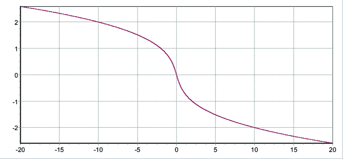
Figure 1: The numerical simulation for the function $U(t,z)$ corresponding to $t=-7$.

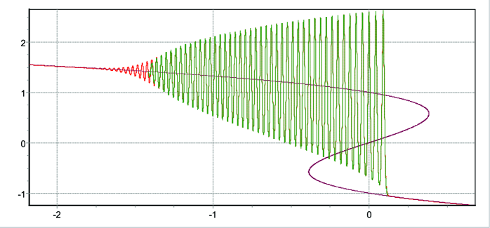
Figure 2: The numerical simulation for the function $U(t,z)$ corresponding to $t=20$ and root of equation $z-\Lambda+\Lambda^{3}=0$.

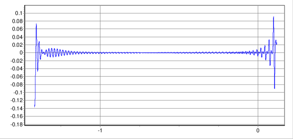
Figure 3: The difference between the numerical solutions and asymptotic for $U(t,z)$ for $t=20$.

To this end we have written a special program. The results of numerical simulations are presented in Figures 1 – 3.

In Figures 1-2 one can observe numerical solutions for function $U(t,z)$ for negative and positive value $t$. It can be shown that function $U(t,z)$ for negative value $t$ practically councide with the root of the equation $\Lambda^{3}+\Lambda=-z$.

In Figure 3 the difference between these solutions is shown. Both figures correspond to $t=20$. The constant $s_{0}$ has proved to be equal to $3.1254\approx\pi$. The difference between two solutions is a multiple of $t^{-1.77}\approx t^{-7/4}$ which agrees with the order of the first correction in formula (2.2).

We believe that the constant $s_{0}$ just amounts to $\pi$ and the small difference is caused by a computation error.

Figure 3 makes it evident that the error increases for $z$ close to $-\sqrt{2}$ and $\sqrt{10}/27$. This manifests the nonuniform character of the constructed asymptotic formula in the entire domain of the variable $z$. In neighbourhoods of the leading and trailing wave front sets one should construct other asymptotic formulas which can be made consistent with asymptotic expansion (2.2), as it is described in [18].

4 Reduction of equations to standard form

To start with, we bring the equations obtained in [16] to a simpler form. These are

$$z-Y_{j}+Z_{j}=0$$

for $j=1,2,3$, where

$$\begin{array}[]{rclrclrcl}Y_{1}&\!\!=\!\!&\displaystyle\frac{1}{3}S_{1}\!+\!\frac{2}{3}\frac{l_{1}\!-\!l_{2}}{1\!-\!q},&Y_{2}&\!\!=\!\!&\displaystyle\frac{1}{3}S_{1}\!-\!\frac{2}{3}\frac{(l_{1}\!-\!l_{2})(1\!-\!k^{2})}{1\!-\!q\!-\!k^{2}},&Y_{3}&\!\!=\!\!&\displaystyle\frac{1}{3}S_{1}\!+\!\frac{2}{3}\frac{l_{3}\!-\!l_{2}}{q},\\ S_{1}&\!\!=\!\!&l_{1}+l_{2}+l_{3},&S_{2}&\!\!=\!\!&l_{1}l_{2}+l_{2}l_{3}+l_{3}l_{2},&S_{3}&\!\!=\!\!&l_{1}l_{2}l_{3}\\ \end{array}$$

and

$$Z_{j}=\frac{1}{35}\Big{(}V+(3Y_{j}-S_{j})V^{\prime}_{l_{j}}\Big{)}$$

with $V=5S_{1}^{3}-12S_{1}S_{2}+8S_{3}$.

Obviously, one can eliminate two variables from three equations. On eliminating $z$ and $q$ we get an equation for $l_{1}$, $l_{2}$ and $l_{3}$, which does not contain $z$ and $q$. Namely,

$$3\,(l_{1}^{2}+l_{2}^{2}+l_{3}^{2})+2\,(l_{1}l_{2}+l_{2}l_{3}+l_{3}l_{1})-5=0.$$ (4.1)

We now eliminate either of the variables $z$ and $q$ in the equations and use (4.1) to eliminate all powers of $l_{1}$ greater than the first one. Then we get two more equations

$$z = \frac{2}{45}\Big{(}l_{1}(8l_{2}^{2}+4l_{2}l_{3}+8l_{3}^{2}-15)-(l_{2}+l_{3})(24l_{2}^{2}-8l_{2}l_{3}+24l_{3}^{2}-25)\Big{)},$$

$$q = \frac{1}{2}\,\frac{(l_{2}-l_{3})(3l_{2}l_{3}+3l_{3}l_{1}+9l_{3}^{2}-5)}{l_{1}(2l_{2}^{2}+l_{2}l_{3}+2l_{3}^{2}-5)-(l_{2}+l_{3})(6l_{2}^{2}-2l_{2}l_{3}+6l_{3}^{2}-5)}.$$

The system of equations (2.3), (2.7) and (2.8) is equivalent to the system of averaged equations (4.1) and (4) which was obtained in [16] by Whitham’s method. To prove this, we pass in the system of the equation for $C$ in (2.9) and equations (2.10), (2.11) to Whitham’s variables $l_{1}(z)$, $l_{2}(z)$ and $l_{3}(z)$ by

$$\begin{array}[]{rclrclrcl}A&\!\!=\!\!&2\,(l_{3}-l_{1}),&C&\!\!=\!\!&l_{1}+l_{2}-l_{3},&k^{2}&\!\!=\!\!&\displaystyle\frac{l_{2}-l_{1}}{l_{3}-l_{1}}.\end{array}$$

On eliminating $z$ and $q$ from the obtained equations we arrive precisely at (4.1). On eliminating either of $z$ and $q$ and all powers of $l_{1}$ greater than the first one, we get (4), as desired.

5 Conclusion

It should be noted that the value of the phase shift $s_{0}$ derived from the numerical simulation contradicts [3, 4]. From the results of the paper it follows that the function $s(z)$ tends to $\pi/2$, as $z\to z_{l}$. But there is an arithmetical error in formula (17)[3] and in formula (21)[4]. The right calculation with using monodromic date from [19] showed that $s(z)$ tends to $\pi$, and so

$$s(z)\equiv\pi.$$

Acknowledgements  The authors are greatly indepted to V. Adler for first numerical experiments in this problem. The derivation of equation (2.5) without using the averaging method is due to our colleague V. Kudashev. The research of the first author was supported by the DFG grant TA 289/4-1 and by the Program for Supporting Young Scientists, grant MK-2812.2010.1. The first and second authors were also supported by the RFBR 09-01-92436, 10-01-91222.

References

• Gurevich and Pitaevskii [1971] A. V. Gurevich, L. P. Pitaevskii, Breaking of a simple wave in the kinetics of a rarefied plasma, Zh. Eksp. Teor. Fiz. 60 (1971) 2155–2174, [Sov. Phys. JETP 33 (1971) 1159].
• Sagdeev [1964] R. Z. Sagdeev, Collective processes and shock waves in a rarefied plasma, vol. 4 of Problems in Plasma Theory, Atomizdat, Moscow, 20–88, 1964.
• Kudashev and Suleimanov [1996] V. Kudashev, B. Suleimanov, A soft mechanism for the generation of dissipationless shock waves, Phys. Lett. A 221 (1996) 204–208.
• Kudashev and Suleimanov [1964] V. Kudashev, B. Suleimanov, A soft mechanism for the generation of dissipationless shock waves, in: Complex Anal., Diff. Eq., and Appl., III: Diff. Eq., Inst. of Math., Ufa, 98–108, URL http://matem.anrb.ru/e_lib/preprints/BS/bs22.html, 1964.
• Kudashev and Suleimanov [2001] V. R. Kudashev, B. I. Suleimanov, The effect of small dissipation on the onset of one-dimensional shock waves, PMM 65 (2001) 456–466, [J. Appl. Maths Mechs 65 (2001) 441-451].
• Ovsyannikov [1985] L. V. Ovsyannikov, Lagrangian approximations in the theory of waves, Nonlinear Problems in the Theory of Surface and Internal Waves, Novosibirsk, Nauka, 10–77, 1985.
• Suleimanov [1994] B. I. Suleimanov, Generation of dissipationless shock waves and the non-perturbative quantum theory of gravitation, Zh. Eksp. Teor. Fix. 60 (1994) 1089–1097, [JETP 78 (1994) 583-587].
• Bresin et al. [1990] E. Bresin, R. Marinari, G. Parisi, A non-perturbative ambiguity free solution of a string model, Phys. Lett. B 242 (1990) 35–38.
• Moore [1990] G. Moore, Geometry of the string equations, Comm.Math. Phys. 133 (1990) 261–304.
• Douglas et al. [1990] M. Douglas, N. Seiberg, S. Shenker, Flow and instability in quantum gravity, Phys. Lett. B 244 (1990) 381–385.
• Dubrovin [2006] B. A. Dubrovin, On Hamiltonian perturbations of hyperbolic systems of conservation laws II: Universality of critical behaviour, Comm.Math. Phys. 267 (2006) 117–139.
• Dubrovin [1994] B. A. Dubrovin, Hamiltonian PDEs and Frobenius manifolds, UMN 63:6 (1994) 7–18, [Russian Math. Surveys 63 (2008) 999-1010].
• Baikov et al. [1989] V. A. Baikov, R. K. Gazizov, N. K. Ibragimov, Approximate symmetry and formal linearization, Zhurnal Prikladnoi Mekhaniki i Tekhnicheskoi Fiziki 30 (1989) 40–49, [J. Appl. Mech. Tech. Phys. 30 (1989) 204-212].
• Gurevich and Pitaevskii [1973] A. V. Gurevich, L. P. Pitaevskii, Nonstationary structure of a collisionless shock wave, Zhurnal Eksperimental’noi i Teoreticheskoi Fiziki 65 (1973) 590–604, [Sov. Phys. JETP 38 (1974) 291-297].
• Whitham [1965] G. B. Whitham, Non-linear dispersive waves, Proc. R. Soc. Ser. A 283 (1965) 238–261.
• Potemin [1988] G. V. Potemin, Algebro-geometric construction of self-similar solutions of the Whitham equations, UMN 43:5 (1988) 211–212, [Russian Math. Surveys 43 (1988) 252-253].
• Garifullin and Suleimanov [2010] R. N. Garifullin, B. I. Suleimanov, From weak discontinuities to dissipationless shock waves, Zh. Eksp. Teor. Fiz. 137 (2010) 149–165, [JETP 110 (2010) 135-148].
• Il’in [1978] A. M. Il’in, Matching of Asymptotic Expansions of Solutions of Boundary Value Problems, Nauka, Moskow, [Transl. of Math. Monographs, vol. 102, AMS, Providence, RI, 1992], 1978.
• Kapaev [1991] A. A. Kapaev, Weakly nonlinear solutions of the equation $P^{2}_{I}$, Zapiski LOMI 137 (1991) 88–109, [Journal of Mathematical Sciences 74 (1995) 468-481].