The Physics of turbulent and dynamically unstable Herbig-Haro jets

Abstract

The overall properties of the Herbig-Haro objects such as centerline velocity , transversal profile of velocity , flow of mass and energy are explained adopting two models for the turbulent jet. The complex shapes of the Herbig-Haro objects , such as the arc in HH34 can be explained introducing the combination of different kinematic effects such as velocity behavior along the main direction of the jet and the velocity of the star in the interstellar medium. The behavior of the intensity or brightness of the line of emission is explored in three different cases : transversal 1D cut , longitudinal 1D cut and 2D map. An analytical explanation for the enhancement in intensity or brightness such as usually modeled by the bow shock is given by a careful analysis of the geometrical properties of the torus.

Keywords  Pre-main sequence objects, young stellar objects (YSO’s) and protostars (T Tauri stars, Orion population, Herbig-Haro objects, Bok globules, bipolar outflows, cometary nebulae, etc.; Jets, outflows, and bipolar flows

1 Introduction

The Herbig-Haro objects , in the following HH , are on the short distances from the central source collimated patches of nebulosity associated with a central very young star; the name derives from the first two astronomer which studied them in details , see Herbig (1950); Haro (1952). The HH are observed in the various band of the electromagnetic spectrum : in the radio , see Rodríguez and Reipurth (1989); Curiel et al. (1989); Anglada et al. (1992); Curiel et al. (1993); Rodriguez and Reipurth (1994) ; in the infrared see Reipurth and Aspin (1997); Reipurth, Devine, and Bally (1998); Chrysostomou et al. (2000); Davis, Smith, and Eislöffel (2000); Davis et al. (2002); Takami et al. (2005, 2006); in the optical see Schwartz et al. (1988); Rolph, Scarrott, and Wolstencroft (1990); Scarrott et al. (1990); Bohm, Raga, and Binette (1991); Uchida et al. (1992); Gómez, Whitney, and Wood (1998); Masciadri and Raga (2001); in the ultraviolet Dopita, Binette, and Schwartz (1982); Cameron and Liseau (1990); Bohm, Raga, and Binette (1991); Boehm, Scott, and Solf (1991); Boehm, Noriega-Crespo, and Solf (1993) ; in the X-ray see Pravdo and Angelini (1993); Raga, Noriega-Crespo, and Velázquez (2002). The HH’s are also observed through emission-line spectra . We remember that the astronomers observe both the forbidden emission lines from low ionization species , $[SII]$ and $[OI]$ as well as ionization lines such as $[OIII]$ and $[NeIII]$, see Hartigan and Morse (2007).

On long distances from the central source the HH are curved, see Salas, Cruz-Gonzalez, and Porras (1998); Bally and Reipurth (2001); Bally et al. (2006). From a theoretical point of view the apparent deceleration of HH34 has been modeled by the interaction of a fragmented jet with the surrounding environment, see Cabrit and Raga (2000). The theoretical problem of the curvature of the HH objects has been attached adopting an HH jet/counterjet system that is immersed in an isotropic stellar wind ,Raga et al. (2009), or discussing the properties and similarities of the laboratory and astrophysical flows, see Ciardi et al. (2008) and Hartigan et al. (2009). The already cited models concerning the HHs leave a series of questions unanswered or partially answered:

• Which are the laws of motion that regulate the propagation of HHs in the Interstellar Medium  ?

• Is it possible to model the main physical properties of HHs such as matter entertainment or mechanical luminosity ?

• Can we model the bending of the HHs at the light of the known rules of the kinematics ?

• Can we model the intensity or brightness behavior along the HHs using different models ?

In order to answer these questions Section 2 reports the astronomical data of two HH objects. Section 3 reports two physical theories on turbulent jets which are converted in astrophysical equations in Section 3. Complex phenomena such as jet’s bending and train of knots are explained in Section 5 adopting the composition of different kinematic effects and the theory of the Kelvin-Helmholtz instabilities . A set of models for the intensity or brightness of HH’s which arise from geometrical arguments are explored in Section 6. Section 7 analyzes a model for the intensity or brightness of HHs as given by a linear and a non linear relationship between emission coefficient $j$ and turbulent power.

2 The astronomical observations

This section presents the astronomical data of HH1 and HH34.

2.1 The inner part of HH1

The collimated jet HH1 has been observed in different astronomical wavelengths such as $[FeII]$ by Reipurth et al. (2000) , near infrared by Davis et al. (2000) , far infrared by Molinari and Noriega-Crespo (2002) , optical/infrared by Nisini et al. (2005) , $H\alpha$ by Riera et al. (2005) , $UV$ by Li et al. (2007) and $FeII$/$H2$ by Garcia Lopez et al. (2008).

HH1 is part of the complex HH 1/2 that covers $3^{\prime}$ with its brightest components. The distance of this complex is $460~{}pc$, see Molinari and Noriega-Crespo (2002); Garcia Lopez et al. (2008).

The length of the jet , $L_{HH1}$ , measured from the central source , VLA1 , to the knot A is according to Nisini et al. (2005)

$$L_{HH1}=22^{\prime\prime}=0.049\;D_{460}\quad pc\quad,$$ (1)

where $D_{460}$ is the distance in units of 460 $pc$ , see Table 2 in Nisini et al. (2005). The initial diameter $d_{i}$ (measured at the knot L-I) and the final diameter $d_{f}$ (measured at the knot A ) are , according to Table 3 in Nisini et al. (2005)

$$d_{i}=2\times 0.1^{\prime\prime}=0.000446\;D_{460}\quad pc$$

$$d_{f}=2\times 0.5^{\prime\prime}=0.00223\;D_{460}\quad pc\quad.$$ (2)

The averaged radius of inner part HH1 is $\overline{r}=0.3^{\prime\prime}$ and 9 blobs characterize the structure. The half opening angle , $\alpha/2$ , is

$$\frac{\alpha}{2}=\arctan\frac{d_{f}/2-d_{i}/2}{L_{HH1}}=0.0181~{}rad=1.041~{}^{\circ}\quad.$$ (3)

With these data the laboratory parameter $x/d$ is is

$$\frac{x}{d}=\frac{L_{HH1}}{d_{i}}=110\quad,$$ (4)

where $x$ represents the jet’s length and $d$ the nozzle’s diameter .

2.2 HH34 the giant jet

HH34 constitutes the archetypal bipolar collimated jet from a young star and has been carefully studied in deep $H\alpha$ and $[SII]$ with the Wide Field Planetary Camera 2 on board of the Hubble Space Telescope and at the Gemini Observatory, see Reipurth et al. (2002); Beck et al. (2007).

According to the data on HH34 as suggested in Masciadri et al. (2002) and Reipurth and Raga (1999) the distance is $460~{}pc$, the length of the jet (arc comprised) , $L_{HH34}$ , is

$$L_{HH34}=1.5\,pc\quad or\quad 4.62\,10^{18}~{}cm\quad,$$ (5)

the initial jet’s diameter is

$$d_{i}=9.7\,10^{-4}pc\quad or\quad 6\times 10^{15}~{}cm\quad.$$ (6)

The ratio $x/d$, takes the value

$$\frac{x}{d}=\frac{L_{HH34}}{d_{i}}=773\quad.$$ (7)

A detailed study of the inner part of HH34 shows a well collimated jet , see Beck et al. (2007) , which means an opening angle of few degree , i.e. $\alpha=2.86^{\circ}$ (measure of the author). Making reference to Figure 3 in Reipurth et al. (2002) the inner part of HH34 has an averaged radius of $0.5^{\prime\prime}$, a length of $27^{\prime\prime}$ and twelve blobs .

3 The turbulent jet

This Section reports known and new formulas on turbulent jets. We selected the modern approach to turbulent round jets, see Pope (2000) and the classical approach of Landau (1987). These two approaches were already used to model the extragalactic jets , see Zaninetti (2007, 2009).

3.1 The exact solution

The theory of turbulent round jets can be found in different textbooks. The more important formulas are now reviewed as extracted from chapter V in Pope (2000) ; similar results can be found in Bird, Stewart, and Lightfoot (2002) and in Schlichting et al. (2004). We start with the centerline velocity $U_{0}(x)$ , equation (5.6) in Pope (2000) , as measured in the laboratory experiments :

$$\frac{U_{0}(x)}{U_{1}}=\frac{B}{x/d}\quad,$$ (8)

here $x$ denotes the main direction , $d$ is the diameter of the nozzle, $B$ is a constant derived in the laboratory that takes the value 5.8, and $U_{1}$ is the initial jet’s velocity. The solution of the mean velocity $<U>$ , equation (5.100) in Pope (2000) , along the main direction is

$$<U>=U_{1}8a_{T}\nu_{T}\bigl{(}\frac{d}{x}\bigr{)}\frac{1}{(1+a_{T}\eta^{2})^{2}}\quad,$$ (9)

where $\eta=\frac{r}{x}$ , $r$ is the radius of the jet at $x$, $a_{T}$ is a constant and $\nu_{T}$ is the turbulent viscosity. The viscosity , equation (5.104) in Pope (2000) , is

$$\nu_{T}=\frac{S}{8(\sqrt{2}-1)}\quad,$$ (10)

and $a_{T}$, equation (5.18) in Pope (2000), is

$$a_{T}=\frac{(\sqrt{2}-1)}{S^{2}}\quad,$$ (11)

where $S$ is connected with the opening angle $\alpha$ through the following relationship

$$S=\tan\frac{\alpha}{2}\quad.$$ (12)

The production of turbulent kinetic energy in the boundary layer approximation , equation (5.145) in Pope (2000) , is

$${\mathcal{P}}={\nu_{T}(\frac{\partial<U>}{\partial y}})^{2}\quad,$$ (13)

where $y$ is a Cartesian coordinate that can be identified with $r$, the perpendicular distance from the centerline and the units are $\frac{erg}{s\,cm^{3}}$ . The flow rate of mass $m(x)$ is , see equation (5.68) in Pope (2000) ,

$$\dot{m}(x)=2\pi\rho(b_{1/2}(x))^{2}U_{0}(x)\times\int_{0}^{\infty}\xi f(\xi)d\xi\quad,$$ (14)

where

$$\xi=\frac{r}{b_{\frac{1}{2}}(x)}\quad,$$ (15)

and

$$f(\xi)=\frac{1}{(1+A\xi^{2})^{2}}\quad,$$ (16)

where $A$ is a constant that will be later defined and $b_{\frac{1}{2}}$ is the value of the radius at which the velocity is half of the centerline value. The jet draws matter from the surrounding mass of fluid. Hence, the mass of fluid carried by the jet increases with the distance from the source. The flow rate of kinetic energy $E(x)$ is , see equation (5.69) in Pope (2000) ,

$$\dot{E}(x)=\frac{\pi\rho}{b_{\frac{1}{2}}(x)}(b_{\frac{1}{2}}(x)U_{0}(x))^{3}\times\int_{0}^{\infty}\xi(f(\xi))^{3}d\xi\quad,$$ (17)

which has units of $\frac{erg}{s\,cm^{3}}$ .

The previous formulas are exactly the same as in Pope (2000); we now continue toward the astrophysical applications. The self-similar solution for the velocity , equation (9) , can be re-expressed introducing the half width $x=b_{\frac{1}{2}}/S$

$$<U>=U_{1}8a_{T}\nu_{T}\bigl{(}\frac{d}{x}\bigr{)}\frac{1}{(1+A(\frac{r}{b_{\frac{1}{2}}})^{2})^{2}}\quad,$$ (18)

where $A=\sqrt{2}-1$ . From the previous formula is clear the universal scaling of the profile in velocity that is reported in Figure 1.

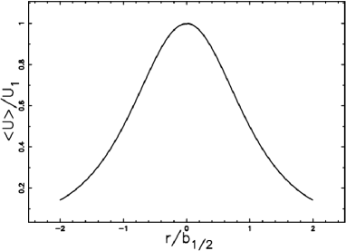
Fig. 1 : Mean velocity profile vs. channel radius in a turbulent round jet. The velocity distribution is a function growing from zero (at the wall of the channel) to a maximum value in the central region. The experimental data at $Re$ $\approx$ $10^{5}$ and $x/d$= 40 , 60, 75 and 97.5 can be found in Wygnanski Fiedler 1969.

From a careful inspection of the previous formula it is clear that the variable $x$ should be expressed in $d$ units (the nozzle’s diameter) in order to reproduce the laboratory results. In doing so we should find the constant $k$ that allows us to deduce $B$

$$B=k\times 8a_{T}\nu_{T}\quad.$$ (19)

Table 1 reports a set of $S$ , $B$ and $\nu_{T}$ for different opening angles $\alpha$ .

Table 1 : Parameters of the turbulent jet when $k$ = 0.54 .

$\displaystyle\hskip 0.0pt{\begin{array}[]{ccccc}\hline\cr\hline\cr\vskip 6.0pt\cr\alpha[rad]&\alpha[degree]&S&B&\nu_{T}\\ \vskip 6.0pt\cr\hline\cr\vskip 6.0pt\cr 0.035&2&0.017&30.96&0.0052\\ 0.087&5&0.043&12.37&0.013\\ 0.14&8&0.07&7.72&0.021\\ 0.185&10.64&0.093&5.79&0.028\\ 0.261&15&0.131&4.1&0.039\\ 0.343&20&0.17&3.06&0.053\\ 0.436&25&0.22&2.43&0.067\\ 0.523&30&0.26&2.01&0.08\\ \vskip 6.0pt\cr\vskip 6.0pt\cr\hline\cr\hline\cr\end{array}}$

The assumption here used is that $k$ is the same for different angles. The velocity expressed in these practical units is

$$<U>=BU_{1}\frac{d}{x}\frac{1}{(1+A~{}(\frac{r}{b_{\frac{1}{2}}})^{2})^{2}}\quad.$$ (20)

This formula can be used for $x$ expressed in $d$-units when $x>B$.

The first derivative of the profile in velocity as given by formula (20) with respect to the radius is

$$\frac{d}{dr}<U>=$$

$$U_{1}\times\frac{-4\,\left(\sqrt{2}-1\right){\it A~{}k}\,{{\it{b_{\frac{1}{2}}}}}^{6}A~{}rd}{\tan\left(\frac{\alpha}{2}\right)\left(\sqrt{2}-1\right)x\left({{\it{b_{\frac{1}{2}}}}}^{2}+A~{}{r}^{2}\right)^{3}{{\it{b_{\frac{1}{2}}}}}^{2}}\quad.$$ (21)

The production of turbulent kinetic energy is

$${\mathcal{P}}=\nu_{T}U_{1}^{2}\times$$

$$\times\frac{2\,\left(\sqrt{2}-1\right)^{2}{{\it A~{}k}}^{2}{{\it{b_{\frac{1}{2}}}}}^{12}{A~{}}^{2}{r}^{2}d^{2}}{\tan\left(\frac{\alpha}{2}\right)\left(\sqrt{2}-1\right)^{3}{x}^{2}\left({{\it{b_{\frac{1}{2}}}}}^{2}+A~{}{r}^{2}\right)^{6}{{\it{b_{\frac{1}{2}}}}}^{4}}\quad.$$ (22)

It is interesting to note that the maximum of $\mathcal{P}$ , is at

$$r=\frac{1}{\sqrt{5}}\frac{b_{\frac{1}{2}}}{\sqrt{A~{}}}=0.69{b_{\frac{1}{2}}}\quad.$$ (23)

In these practical units the flow rate of mass , equation (14), becomes

$$\dot{m}(x)=\frac{\pi\,\rho\,x\left(\tan\left(\frac{\alpha}{2}\right)\right)^{3}{\it U_{1}}\,d}{\sqrt{2}-1}\quad,$$ (24)

and flow of kinetic energy , equation (17) , is

$$\dot{E}(x)=\frac{{d}^{3}{{\it U_{1}}}^{3}\left(\tan\left(\frac{\alpha}{2}\right)\right)^{5}\rho\,\pi}{10\,\left(\sqrt{2}-1\right)x}\quad.$$ (25)

A more sophisticated approach makes extensive use of a statistical mass-averaging technique for compressible turbulent flow, see Favre, A. (1969); Bicknell (1984).

3.2 The simple solution

We now outline the conservation of the momentum flux in a ”turbulent jet” , see Landau (1987) . The initial point is characterized by the following section

$$A_{0}=\pi~{}r_{0}^{2}\quad.$$ (26)

On introducing $\alpha$ ,the opening angle , $x_{0}$ ,the initial position on the $x$–axis, and $v_{0}$ , the initial velocity , the section $A$ at position $x$ is

$$A(x)=\pi\bigl{(}{\it r_{0}}+\left(x-{\it x_{0}}\right)\tan\left(\frac{\alpha}{2}\right)\bigr{)}^{2}\quad.$$ (27)

The conservation of the total momentum flux states that

$$\rho v_{0}^{2}A_{0}=\rho v(x)^{2}A(x)\quad,$$ (28)

where $v(x)$ is the velocity at position $x$ . Due to the turbulent transfer, the density $\rho$ is the same on both the two sides of equation (28). The trajectory of the jet as a function of the time is easily deduced from equation (28)

$$x=$$

$${\frac{{\it x_{0}}\,\tan\left(\frac{\alpha}{2}\right)-{\it r_{0}}+\sqrt{{\it r_{0}}\,\left({\it r_{0}}+2\,\tan\left(\frac{\alpha}{2}\right){\it v_{0}}\,t\right)}}{\tan\left(\frac{\alpha}{2}\right)}}\quad.$$ (29)

The velocity as function of the time turns out to be

$${\it v(t)}={\frac{{\it v_{0}}\,{\it r_{0}}}{\sqrt{{\it r_{0}}\,\left({\it r_{0}}+2\,\tan\left(\frac{\alpha}{2}\right){\it v_{0}}\,t\right)}}}\quad.$$ (30)

The flow rate of mass and kinetic energy are respectively

$$\dot{m}(x)=\pi r^{2}\rho v\quad,$$ (31)

$$\dot{E}(x)=\pi r^{2}\frac{1}{2}\rho v^{2}\quad,$$ (32)

where $r$ and $v$ are the momentary radius and velocity of the jet.

4 The physics of HH’s

This Section reports the centerline velocity, the equation of motion , the flow of mass and the flow of energy for the two turbulent models here considered.

4.1 The exact solution

Equation (8) allows us to deduce the centerline velocity of the turbulent astrophysical jet

$$u_{0}(x)=\frac{0.5409\,{\it u_{100}}\,{\it d_{1}}}{\tan\left(0.00872\,{\it\alpha_{deg}}\right){\it x_{1}}}\frac{Km}{sec}\quad,$$ (33)

where $\alpha_{deg}$ is the opening angle expressed in degree, $u_{100}$ is the initial velocity expressed in units of $100\frac{km}{s}$ , $u_{100}=\frac{U_{1}[km/s]}{100}$ , $d_{1}$ is the diameter of the nozzle in $pc$ units and $x_{1}$ is the length of the jet in $pc$ units.

The previous equation allows us to deduce the equation of motion for a turbulent astrophysical jet ,

$$x(t)=1.050\,\sqrt{{\frac{{\it u_{100}}\,{\it d_{1}}\,{\it t_{4}}}{\tan\left(0.00872\,{\it\alpha_{deg}}\right)}}}\;pc\quad,$$ (34)

where $t_{4}$ = $t[yr]/(10^{4})$ . The radius of the turbulent jet is

$$r(x)=[\frac{d_{1}}{2}+x(t)\tan(\frac{\alpha_{deg}}{2})]pc\quad.$$ (35)

Combining equations (33) , (34) and (34) is possible to deduce the velocity of the HH object , for example HH34 , as function of the time see Figure 2.

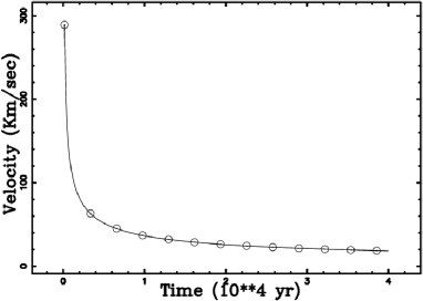
Fig. 2 : Velocity of HH34 in $\frac{Km}{s}$ versus time in $t_{4}$ units when $\alpha=2.86^{\circ}$ , $u_{100}=6.5$ , $d_{1}=1.94\,10^{-3}$ and $x_{1}=1.49$.

The power released in the turbulent cascade is

$$\epsilon(r,x)=$$

$$\frac{2\,\left(\sqrt{2}-1\right)^{2}{{\it k}}^{2}{{\it b_{\frac{1}{2}}}}^{12}{A~{}}^{2}{r}^{2}}{\tan\left(\frac{\alpha}{2}\right)\left(\sqrt{2}-1\right)^{3}\left({{\it b_{\frac{1}{2}}}}^{2}+A~{}{r}^{2}\right)^{6}{{\it b_{\frac{1}{2}}}}^{4}}$$

$$\times(\frac{d_{1}}{x_{1}})^{2}\quad.$$ (36)

The flow rate of mass , see equation (24) , as expressed in these astrophysical units is

$$\dot{m}(x)=$$

$$0.1910\,\mu\,{\it n_{0}}\,{\it x_{1}}\,\left(\tan\left(0.008725\,{\it\alpha_{deg}}\right)\right)^{3}{\it u_{100}}{\it d_{1}}\,$$

$$\frac{{\mathcal{M}}_{\sun}}{\mbox{year4}},$$ (37)

where $n_{0}$ is the number density expressed in particles $\mathrm{cm}^{-3}$  (density $\rho=n_{0}$m, where $m=\mu m_{\mathrm{H}}$) , $\mu$ is the mean molecular weight (see McCray and Layzer (1987) suggests $\mu$=1.4 ) , $m_{\mathrm{H}}$ is the hydrogen mass , ${\mathcal{M}}_{\sun}$ is the mass of the sun and $yr4$ are $10^{4}~{}year$. On introducing the solar system abundances , $N(El)$ , where $El$ represents the considered element , see Table 2 in Lodders (2003) , and the time expressed in $year$ we obtain

$$\dot{m}(x)=$$

$$1.9\times 10^{-5}\,\mu\,{\it n_{0}}\,{\it x_{1}}\,\left(\tan\left(0.008725\,{\it\alpha_{deg}}\right)\right)^{3}{\it u_{100}}\,{\it d_{1}}$$

$$\frac{N(El)}{N(H)}\quad\frac{{\mathcal{M}}_{\sun}}{\mbox{year}}\quad,$$ (38)

where $N(H)$ is the Hydrogen solar system abundance.

As an example when the $Fe$ is considered we obtain

$$\dot{m}(x)=$$

$$6.59\times 10^{-10}\,\mu\,{\it n_{0}}\,{\it x_{1}}\,\left(\tan\left(0.008725\,{\it\alpha_{deg}}\right)\right)^{3}{\it u_{100}}\,{\it d_{1}}$$

$$\quad\frac{{\mathcal{M}}_{\sun}}{\mbox{year}}\quad,$$ (39)

$$case~{}of~{}Fe$$

where $\frac{N(Fe)}{N(H)}=\frac{8.380\times 10^{5}}{2.431\times 10^{10}}$ ,see Table 2 in Lodders (2003).

A comparison of the previous formula can be done with ${\dot{\mathcal{M}}}([FeII])$ that in HH1 varies between $2.2\times 10^{-7}{\mathcal{M}}_{\sun}yr^{-1}$ and $2.8\times 10^{-9}{\mathcal{M}}_{\sun}yr^{-1}$ , see Table 3 in Nisini et al. (2005).

The flow of energy ,equation (25), in these astrophysical units is

$$\dot{E}(x)=$$

$$\frac{{1.203\times 10^{34}}\,\mu\,{\it n_{0}}\,\left(\tan\left(0.00872\,{\it\alpha_{deg}}\right)\right)^{5}{{\it u_{100}}}^{3}{{\it d_{1}}}^{3}}{{\it x_{1}}}$$

$$\quad\frac{ergs}{s}\quad.$$ (40)

The analysis makes extensive use of Favre’s (1969) statistical mass-averaging technique for compressible turbulent flow

4.2 The simple solution

Equation (30) allows us to deduce the centerline velocity in the simple case

$$u_{0}(x)=$$

$$\frac{1.021{\it u_{100}}{\it d_{1}}}{{\it d_{1}}+2\tan\left(0.00872{\it\alpha_{deg}}\right){\it x_{1}}-{\it d_{1}}\tan\left(0.00872{\it\alpha_{deg}}\right)}$$

$$\frac{Km}{sec}\quad.$$ (41)

The astrophysical version of the equation of motion,formula (29), is

$$x(t)=0.5{\it d_{1}}-0.5{\frac{{\it d_{1}}}{\tan\left(0.00872{\it\alpha_{deg}}\right)}}+$$

$$0.707{\frac{\sqrt{0.5{{\it d_{1}}}^{2}+2.042{\it d_{1}}\tan\left(0.00872{\it\alpha_{deg}}\right){\it u_{100}}{\it t_{4}}}}{\tan\left(0.00872{\it\alpha_{deg}}\right)}}.$$ (42)

The flow rate of mass , see equation (31) , is

$$\dot{m}(x)=0.01259\,(0.5\,{\it d_{1}}+\tan\left(0.00872\,{\it\alpha_{deg}}\right){\it x_{1}}$$

$$-0.5\,{\it d_{1}}\,\tan\left(0.00872\,{\it\alpha_{deg}}\right)){\it d_{1}}\,{\it u_{100}}\,\mu\,{\it n_{0}}\,{}\frac{{\mathcal{M}}_{\sun}}{\mbox{year4}}\quad.$$ (43)

The flow of kinetic energy ,equation (32), is

$$\dot{E}(x)=\frac{{6.231\times 10^{33}}\,\mu\,{\it n_{0}}\,{{\it u_{100}}}^{3}{{\it d_{1}}}^{3}}{{\it d_{1}}+2.0\,\tan\left(0.00872\,{\it\alpha_{deg}}\right){\it x_{1}}}\quad\frac{ergs}{s}\quad.$$ (44)

5 Complex trajectories

This section reports the kinematic effects that lead to complicate trajectories as well an explanation for the train of knots which are visible in the first part of the HH objects.

5.1 The precessing jets

The wide spectrum of observed morphologies that characterizes the HH objects can be due to the kinematic effects as given by the composition of the velocities of different effects such as decreasing jet velocity , jet precession and proper velocity of the host star in the interstellar medium (ISM). Of particular interest is the evaluation of various matrices that will enable us to cause a transformation from the inertial coordinate system of the jet to the coordinate system in which the host star is moving in space. The various coordinate systems will be ${\bf x}$=$(x,y,z$) , ${\bf x}^{(1)}$=$(x^{(1)},y^{(1)},z^{(1)})$ , $\ldots$ ${\bf x}^{(3)}$=$(x^{(3)},y^{(3)},z^{(3)})$. The vector representing the motion of the jet is represented by the following $1\times 3$ matrix

$$G=\left[\begin{array}[]{c}x\left(t\right)\\ \vskip 12.5pt\cr 0\\ \vskip 12.5pt\cr 0\end{array}\right]\quad,$$ (45)

where the jet motion L(t) is considered along the x-axis.

The jet axis, $x$, is inclined at an angle $\Psi_{prec}$ relative to an axis $x^{(1)}$ and therefore the $3\times 3$ matrix, representing a rotation through the z axis, is given by:

$$F=\left[\begin{array}[]{ccc}\cos\left(\Psi_{{{\it prec}}}\right)&-\sin\left(\Psi_{{{\it prec}}}\right)&0\\ \vskip 12.5pt\cr\sin\left(\Psi_{{{\it prec}}}\right)&\cos\left(\Psi_{{{\it prec}}}\right)&0\\ \vskip 12.5pt\cr 0&0&1\end{array}\right]\quad.$$ (46)

From a practical point of view $\Psi_{prec}$ can be derived by measuring the half opening angle of the maximum of the sinusoidal oscillations that characterizes the jet.

If the jet is undergoing precession around the $x^{(1)}$ axis, $\Omega_{prec}$ can be the angular velocity of precession expressed in $\mathrm{radians}$ per unit time ; $\Omega_{prec}$ is computed from the optical maps by measuring the number of sinusoidal oscillations that characterize the jet. The transformation from the coordinates ${\bf x}^{(1)}$ fixed in the frame of the precessing jet to the non-precessing coordinate ${\bf x}^{(2)}$ is represented by the $3\times 3$ matrix

$$P=\left[\begin{array}[]{ccc}1&0&0\\ \vskip 12.5pt\cr 0&\cos\left(\Omega_{{{\it prec}}}t\right)&-\sin\left(\Omega_{{{\it prec}}}t\right)\\ \vskip 12.5pt\cr 0&\sin\left(\Omega_{{{\it prec}}}t\right)&\cos\left(\Omega_{{{\it prec}}}t\right)\end{array}\right]\quad.$$ (47)

As an example Figure 3 reports the precessing jet applied to HH34.

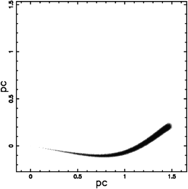
Fig. 3 : Continuous three-dimensional trajectory of HH34: the three Eulerian angles characterizing the point of view are $\Phi$= 0 ^∘ , $\Theta$= 0 ^∘ and $\Psi$= 0 ^∘. The precession is characterized by the angle $\Psi_{prec}$= 10 ^∘ and by the angular velocity $\Omega_{prec}$= 36.00 [${}^{\circ}/10^{4}\mathrm{year}$]. The physical parameters characterizing the jet motion are : $u_{100}=6.5$, $t_{4}=4$ , $x_{1}=1.49$ , $d_{1}=9.7\,10^{-4}$ and $\alpha_{0}$= 2.86 ^∘.

The last translation represents the change of framework from $\bf(x^{(2)})$, which is co-moving with the host star, to a system $\bf(x^{(3)})$ in comparison to which the host star is in a uniform motion. In the laboratory experiments the velocity of the host star is replaced by a wind , see Figure 3 in Ciardi et al. (2008). The relative motion of the origin of the coordinate system $(x^{(3)},y^{(3)},z^{(3)})$ is defined by the Cartesian components of the star velocity $v_{x},v_{y},v_{z}$, and the required $1\times 3$ matrix transformation representing this translation is:

$$B=\left[\begin{array}[]{c}v_{{x}}t\\ \vskip 12.5pt\cr v_{{y}}t\\ \vskip 12.5pt\cr v_{{z}}t\end{array}\right]\quad.$$ (48)

On assuming, for the sake of simplicity, that $v_{x}$=0 and $v_{z}$=0, the translation matrix becomes:

$$B=\left[\begin{array}[]{c}0\\ \vskip 12.5pt\cr v_{{y}}t\\ \vskip 12.5pt\cr 0\end{array}\right]\quad.$$ (49)

In other words, the direction of the star motion in the ISM and the direction of the jet are perpendicular. From a practical point of view the star velocity can be measured by dividing the length of the star in a direction perpendicular to the initial jet velocity by the lifetime of the jet. The final $1\times 3$ matrix $A$ representing the “motion law” can be found by composing the four matrices already described

$$A=B+(P\cdot F\cdot G)$$

$$= \left[\begin{array}[]{c}\cos\left(\Psi_{{{\it prec}}}\right)x\left(t\right)\\ \vskip 12.5pt\cr v_{{y}}t+\cos\left(\Omega_{{{\it prec}}}t\right)\sin\left(\Psi_{{{\it prec}}}\right)x\left(t\right)\\ \vskip 12.5pt\cr\sin\left(\Omega_{{{\it prec}}}t\right)\sin\left(\Psi_{{{\it prec}}}\right)x\left(t\right)\end{array}\right]\quad.$$ (53)

The three components of the previous $1\times 3$ matrix $A$ represent the jet motion along the Cartesian coordinates as given by the observer that sees the star moving in a uniform motion. As an example Figure 4 reports the effect of inserting the star’s velocity on the precessing HH34 as plotted in Figure 3.

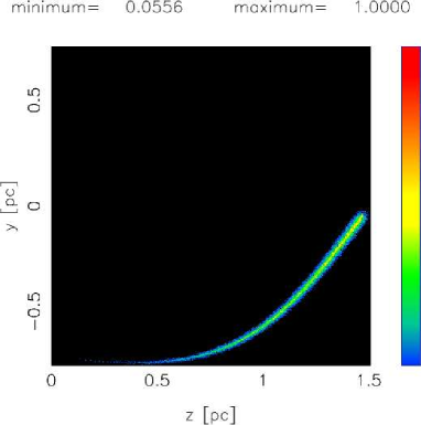
Fig. 4 : Continuous three-dimensional trajectory of HH34: the three Eulerian angles characterizing the point of view are $\Phi$= 0 ^∘ , $\Theta$= 0 ^∘ and $\Psi$= 0 ^∘. The precession is characterized by the angle $\Psi_{prec}$= 10 ^∘ and by the angular velocity $\Omega_{prec}$= 36.00 [${}^{\circ}/10^{4}\mathrm{year}$]. The star has velocity $v_{y}=11.19\frac{Km}{s}$. The physical parameters characterizing the jet motion are : $u_{100}=6.5$, $t_{4}=4$ , $x_{1}=1.49$ , $d_{1}=9.7\,10^{-4}$ and $\alpha_{0}$= 2.86 ^∘. Here the plane of the trajectory is perpendicular to the observer . The two Cartesian axis are in $pc$ and the integral operation which allows to build the image is performed on cubic grid of $1200^{3}$ pixels.

The fifth matrix allows to model the point of view of the observer through the matrix $E$ representing the three Eulerian angles which characterizes the point of view of the observer, $\Theta,\Phi,\Psi$ , see Goldstein, Poole, and Safko (2002) . The product $E\cdot A$ is not reported for space problem and Figure 5 reports the same as Figure 4 , but from a particular point of view. In other words the particular point of view can produce complex projected patterns of a simple basic trajectory as represented by Figure 4. A comparison of Figure 5 should be done with the image of HH34 as available at
http://antwrp.gsfc.nasa.gov/apod/ap991129.html
made with the VLT by the FORS Team or Figure 1 in Reipurth et al. (2002) which has a field of $4.5^{\prime}\times 5^{\prime}$.

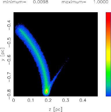
Fig. 5 : Continuous three-dimensional trajectory of HH34: the three Eulerian angles characterizing the point of view are $\Phi$= 290 ^∘ , $\Theta$= 180 ^∘ and $\Psi$= 18 ^∘. The precession is characterized by the angle $\Psi_{prec}$= 10 ^∘ and by the angular velocity $\Omega_{prec}$= 36.00 [${}^{\circ}/10^{4}\mathrm{year}$]. The star has velocity $v_{y}=11.19\frac{Km}{s}$. The physical parameters characterizing the jet motion are : $u_{100}=6.5$, $t_{4}=4$ , $x_{1}=1.49$ , $d_{1}=9.7\,10^{-4}$ and $\alpha_{0}$= 2.86 ^∘. The image is here reported as a theoretical 2D surface brightness of emission, the two Cartesian axis are in $pc$ and the integral operation is performed on cubic grid of $1200^{3}$ pixels.

The astrophysical version of the star’s motion as represented by the translation matrix $B$, formula (49), is

$$y=0.01021\,{\it v_{y}}\,{\it t_{4}}\quad,$$ (54)

where $v_{y}$ is expressed in $\frac{Km}{s}$ units and $t_{4}$ = $t[yr]/(10^{4})$ .

The previous equation can be combined with the motion along $x$ as represented by equation (34) in order to find the angle $\beta$ in degree that characterizes the trajectory:

$$\beta=\arctan(\frac{y}{x})=$$

$$57.29\arctan(\frac{0.009718v_{y}\sqrt{{\it t_{4}}}}{\sqrt{\it u_{100}}\sqrt{d_{1}}\sqrt{\tan\left(0.008727{\it\alpha_{deg}}\right)}})~{}~{}^{\circ}.$$ (55)

This angle varies from 0 when $t_{4}$=0 to $23.39^{\circ}$ when $t_{4}$=4 and the parameters of Figure (4) are used.

Is also interesting to point out that a rotation of $90^{\circ}$ around the $y$ axis of the trajectory as reported in Figure 4 makes the jet straight rather than bended.

Analogous results on ballistic jets from precessing sources has been obtained, see Lightfoot and Glencross (1986); Raga (1993).

5.2 The Kelvin-Helmholtz instabilities

The macroscopic phenomena of the jets as the presence of knots and wiggles can be due to the Kelvin-Helmholtz instability (after Kelvin (1871); Helmholtz (1868)) of an axisymmetric flow along the velocity-axis when the wavelengths $\lambda=\frac{2\pi}{k}$ ( $k$ is the wave-vector) are greater than the jet radius $a_{j}$, which is taken to be independent of the position along the jet, see Ferrari, Trussoni, and Zaninetti (1979, 1981); Ray and Ershkovich (1983); Hardee, Clarke, and Howell (1995). The velocity , $U_{0}$, is assumed to be rectangular. The internal ( external ) fluid density is represented by $\rho_{0i}$ ($\rho_{0e}$) , the internal sound velocity is $s_{i}$ and $\nu_{0}$= $\frac{\rho_{0i}}{\rho_{0e}}$. Starting from the equations of motion and continuity, and assuming both fluids to be adiabatically compressible, it is possible to derive and to solve the dispersion relation from a numerical point of view , see Zaninetti (1987).

We then start from observable quantities that can be measured on radio-maps such as the total length $L_{obs}$, the wavelength $\lambda_{obs}^{1}$ of the wiggles ($m$=1) along the jet, the distance $\lambda_{obs}^{0}$ ($m$=0) between knots, and the final offset $\Delta\,L_{obs}$ of the center of the jet.

These observable quantities are identified with the following theoretical variables:

$$\lambda^{1}_{max}=\lambda^{1}_{obs}\quad,$$ (56)

$$\lambda^{0}_{max}=\lambda^{0}_{obs}\quad,$$ (57)

$$A_{0}\exp\bigl{(}\frac{2L_{obs}}{Mt_{ad}a_{j}})=\Delta L_{obs}\quad,$$ (58)

$$nl_{e}=L_{obs}\quad,$$ (59)

where $t_{ad}$ = $t_{min}\cdot s_{i}/a_{j}$ and $A_{0}$ is the amplitude of the perturbed energy. The result is a theoretical expression for $t_{min}$ the minimum time scale of the instability, $\lambda_{max}$ the wavelength connected with the most unstable mode and $l_{e}$ the distance over which the most unstable mode grows by a factor $e$, see Zaninetti (1987). These parameters can then be found through the set of nonlinear equations previously reported. By choosing two objects, HH1 and HH34 the observational parameters can be measured on the optical image, see Table 2.

Table 2 : Parameters of the observed oscillations in HH objects expressed in averaged radius units

$\displaystyle\hskip 0.0pt{\begin{array}[]{lcc}\hline\cr\hline\cr\vskip 6.0pt\cr Geometrical~{}measure&HH1&HH34\\ \vskip 6.0pt\cr\hline\cr\vskip 6.0pt\cr L_{obs}[averaged~{}radius~{}units]&73.3&54\\ \vskip 6.0pt\cr\lambda^{0}_{obs}[averaged~{}radius~{}units]&8.1&4.5\\ \vskip 6.0pt\cr\lambda^{1}_{obs}[averaged~{}radius~{}units]&29.3&27\\ \vskip 6.0pt\cr\Delta L_{obs}[averaged~{}radius~{}units]&1&1\\ \vskip 6.0pt\cr\vskip 6.0pt\cr\hline\cr\hline\cr\end{array}}$

The four nonlinear equations are then solved and the four theoretical parameters are found , see Table 3.

Table 3 : Theoretical parameters from oscillations deduced from the four nonlinear equations

$\displaystyle\hskip 0.0pt{\begin{array}[]{lcc}\hline\cr\hline\cr\vskip 6.0pt\cr Theoretical~{}variable&HH1&HH34\\ \vskip 6.0pt\cr\hline\cr\vskip 6.0pt\cr n&1.22&1.96\\ \vskip 6.0pt\cr M&52.2&26.67\\ \vskip 6.0pt\cr\nu_{0}&325&15.67\\ \vskip 6.0pt\cr A_{0}&0.012&0.017\\ \vskip 6.0pt\cr\hline\cr\hline\cr\end{array}}$

An application of the results for HH1 here obtained is reported in Figure 6 ; the comparison should be done with Figure 1 ($[SII]$) in Reipurth et al. (2000) that covers $\approx$ 14.16 arcseconds. The application to HH34 is reported in Figure 7 and the comparison should be done with Figure 3 in Reipurth et al. (2002) which covers $\approx 30$ arcsec. In both cases the wavelength of the pinch modes ($m=0$) and the oscillations of the helical mode ($m=1$)are those reported in Table 3.

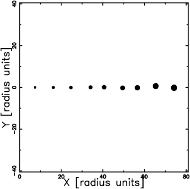
Fig. 6 : Superposition of the pinch mode ($m=0$) on the helical mode ($m=1$) for HH1 in radius units. The parameters are as in Tables 2 and 3.

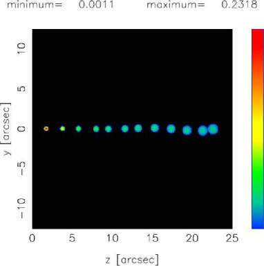
Fig. 7 : Superposition of the pinch mode ($m=0$) on the helical mode ($m=1$) for HH34 in radius units. The parameters are as in Tables 2 and 3. The image is here reported as a theoretical 2D surface brightness of emission, the integral operation is performed on cubic grid of $1200^{3}$ pixels. The intensity or brightness in the spherical blobs ($m=0$) scales as in equation (74).

6 The image from geometry

The transfer equation in the presence of emission only , see for example equation (1.27) in Rybicki and Lightman (1991) or equation (4.9) in Dopita and Sutherland (2003) , is

$$\frac{dI_{\nu}}{ds}=-k_{\nu}\zeta I_{\nu}+j_{\nu}\zeta\quad,$$ (60)

where $I_{\nu}$ is the specific intensity or brightness which has units of $\frac{erg}{s\,cm^{2}\,ster\,Hz}$ , $s$ is the line of sight , $j_{\nu}$ the emission coefficient which has units of $\frac{erg}{s\,cm^{3}\,ster\,Hz}$ , $k_{\nu}$ a mass absorption coefficient, $\zeta$ the mass density at position s and the index $\nu$ denotes the interested frequency of emission. The solution to equation (60) is

$$I_{\nu}(\tau_{\nu})=\frac{j_{\nu}}{k_{\nu}}(1-e^{-\tau_{\nu}(s)})\quad,$$ (61)

where $\tau_{\nu}$ is the optical depth at frequency $\nu$

$$d\tau_{\nu}=k_{\nu}\zeta ds\quad.$$ (62)

We now continue analyzing the case of an optically thin layer in which $\tau_{\nu}$ is very small ( or $k_{\nu}$ very small ) and the density $\zeta$ is substituted with our number density C(s) of particles. Two cases are taken into account : the emissivity is proportional to the number density and the emissivity is proportional to the square of the number density . In the linear case

$$j_{\nu}\zeta=KC(s)\quad,$$ (63)

where $K$ is a constant function.

In the quadratic case

$$j_{\nu}\zeta=K_{2}C(s)^{2}\quad,$$ (64)

where $K_{2}$ is a constant function. This is true for example for free-free radiation from a thermal plasma, see formula (1.219) in Lang (1999) or formula (6.17) in Dopita and Sutherland (2003) .

The intensity is now

$$I_{\nu}(s)=K\int_{s_{0}}^{s}C(s\prime)ds\prime$$ (65)

$$\mbox{optically thin layer}\quad linear~{}case\quad,$$

or

$$I_{\nu}(s)=K_{2}\int_{s_{0}}^{s}C(s\prime)^{2}ds\prime$$ (66)

$$\quad\mbox{optically thin layer}\quad quadratic~{}case\quad.$$

In the Monte Carlo experiments the number density is memorized on a 3D grid ${\mathcal{M}(i,j,k)}$ where $i,j$ and $k$ are indexes varying from 1 to $pixels$ , and the intensity is

$${\it I}\/(i,j)=\sum_{k}\triangle\,s\times{\mathcal{M}}(i,j,k)$$ (67)

$$\quad\mbox{optically thin layer}\quad linear~{}case\quad,$$

or

$${\it I}\/(i,j)=\sum_{k}\triangle\,s\times{\mathcal{M}}(i,j,k)^{2}$$ (68)

$$\quad\mbox{optically thin layer}\quad quadratic~{}case\quad,$$

where $\triangle$s is the spatial interval between the various values of intensity and the sum is performed over the interval of existence of the index $k$. In this grid framework the little squares that characterized by the position of the indexes $i,j$ correspond to a different line of sight. When all the different pixels are viewed together the image is formed. The ensemble of all the pixels can be considered a theoretical surface intensity or a theoretical surface brightness. We now outline a possible source of radiation. The volume emission coefficient of the transition $j_{21}$ is

$$j_{21}=\frac{n_{2}A_{21}h\nu_{21}}{4\pi}\quad,$$ (69)

where level 1 is the lower level , level 2 is the upper level , $n_{2}$ is gas number density , $n_{2}A_{21}$ the rate of photons emitted from a unit volume , $A_{21}$ is the Einstein coefficient for the transition , $h$ is the Planck constant and $\nu_{21}$ the considered frequency, see Hartigan (2008). In the case of optically thin medium the intensity of the emission $I_{21}$ is the integral along the line of sight

$$I_{21}=\int j_{21}dl\quad.$$ (70)

In the case of constant gas number density

$$I_{21}\propto l\quad,$$ (71)

where $l$ is the considered length that in the astrophysical diffuse objects depends from the point of view of the observer. The optically thin layer approximation represents therefore a useful approximation to build models for the intensity of radiation which are comparable to the observed profiles.

We now analyze the behavior of the intensity of a cross section of a jet , the behavior of the maximum intensity at the centerline as a function of the distance from the central source , the intensity of complex morphologies and the sudden increase in intensity as given by the toroidal jet.

6.1 Intensity at a fixed distance

We explore the behavior of the intensity or brightness along the a jet when the distance from the origin ,$y$, is fixed . We assume that the number density $C$ is constant in a cross section of radius $a$ and then falls to 0 , see Figure 8.

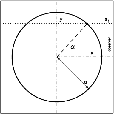
Fig. 8 : The source is represented through a circular section perpendicular to the jet axis. The observer is situated along the x direction, one line of sight is indicated and the angle $\alpha$ is clearly indicated.

The length of sight , when the observer is situated at the infinity of the $x$-axis , is the locus parallel to the $x$-axis which crosses the position $y$ in a Cartesian $x-y$ plane and terminates at the external circle of radius $a$. The locus length is

$$l_{ab}=2\times(\sqrt{a^{2}-y^{2}})\quad;0\leq y<a\quad.$$ (72)

When the number density $C_{m}$ is constant in the cylinder of radius $a$ the intensity or brightness of radiation is

$$I_{0a}=C_{m}\times 2\times(\sqrt{a^{2}-y^{2}})\quad;0\leq y<a\quad,$$ (73)

or

$$I_{0a}=C_{m}\times 2\times a\times\cos(\alpha)\quad;-\frac{\pi}{2}\leq\alpha\leq\frac{\pi}{2}\quad,$$ (74)

that can be named the ”trigonometrical law” for the intensity or brightness . Is interesting to underline that the two previous equations hold for a cylindrical and a conical jet as well for a spherical blob when the number density is constant.

6.2 Centerline Intensity function of the distance

We now explore the behavior of the intensity or brightness at the centerline of the jet as a function of the distance $x$ from the nozzle. From the previous paragraph 6.1 we learned that the maximum intensity or brightness at the centerline of the jet at a fixed distance $x$ is proportional , as a first parameter , to the jet’s diameter $d$ ,

$$I(r=0,x)\propto d(x)C_{m}\propto xC_{m}\quad.$$ (75)

In order to have a constant intensity or brightness along the centerline of the jet as function of $x$ , the number density $C_{m}$ of the emitting particles should decreases as

$$C_{m}(x)\propto\frac{1}{x}\quad.$$ (76)

As a consequence the intensity or brightness

$$I(x)\propto C_{m}\times d\propto\frac{cost}{x}x\quad,$$ (77)

will be constant along the jet. In the framework of the optically thin medium the emitting length will not change but conversely the number density can take the general form

$$C_{m}(x)\propto\frac{1}{x^{s+1}}\quad,$$ (78)

which means that the intensity or brightness scales as

$$I(x)\propto d(x)\frac{1}{x^{s+1}}\propto x^{-s}\quad.$$ (79)

The value of $s$ can found from the scaling of the observed intensity or brightness as function of $x$. As an example of constant intensity or brightness of emission along a knotty jet we report the image of the first part of HH34 where $C_{m}(x)\propto\frac{1}{x^{1+0.15}}$ was chosen ; a comparison should be done with Figure 3 in Reipurth et al. (2002). The relative cut along the jet’s main axis of symmetry, is reported in Figure 9 where $s=0.15$ was used.

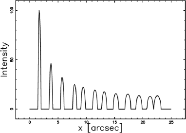
Fig. 9 : Intensity of HH34 represented through a cut in the x-direction (y=0) , parameters as in Figure 7. The intensity or brightness along the cut decreases as $I(x)\propto x^{-0.15}$.

As a practical example the intensity (counts) of $H_{\alpha}$ for HH110 as in Figure 3 of Riera et al. (2003) decreases of a factor $\approx$ 8.6 from the second blob B to the last blob Q. In our simulation of HH34 as reported in Figure 9 the intensity decreases of a factor $\approx$ 8.3 from the first to the last blob.

The 3D algorithm already presented replaces previous efforts based on the 2D random walk , see Figure 7 in Zaninetti (1989) and on the 3D random walk from many injection points , see Figure 8 in Zaninetti (1999).

6.3 Complex Morphologies

The integral operation of the emissivity along the line of sight of a turbulent jet can be performed in an analytical way only in a simple configuration : the jet perpendicular to the observer, see Section 7.1. The concurrency of complex trajectories and a general point of view of the observer characterized by the three Eulerian angles $\Theta$, $\Phi$ and $\Psi$, asks a numerical treatment. We remember that the points that characterize the trajectory of HH34 , see Section 5.1 , are already in such a way that the product $\epsilon(x)\times x$ is nearly constant. This means that the intensity or brightness is nearly constant along the main direction. These points are inserted on a 3D grid made by $pixels^{3}$ points and a sum is performed over one index, see Figure 5.

The enhancement of the intensity or brightness in the previous map where the jet is bending is due to the particular point of view of the observer. Figure  10 reports a cut along the centerline of a jet from which is possible to observe an increase of a factor $\approx$ 5 in the axial intensity or brightness otherwise constant . An analytical evaluation of such increase is reported in Section 6.4.

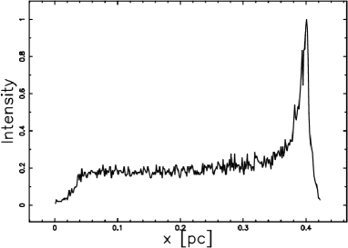
Fig. 10 : Behavior of the intensity or brightness of HH34 at the centerline. Parameters as in Figure 5

Conversely when the plane of the trajectory is perpendicular to the point of view of the observer the enhancement in the intensity or brightness of HH34 is not present , see Figure 4.

6.4 Toroidal Model

The curved shape of a jet of finite cross section is not easy to parametrize. The torus represents a possible model due to the presence of the small radius that characterizes the cross section of the HH object , $r$ , and the great radius $R$ that can be identified with the curvature $k$, $k=1/R$ that characterizes the 3D trajectory. The torus has the following parametric equations:

$$x=\cos(s)\cdot(R+r\cdot\cos(t))$$

$$y=\sin(s)\cdot(R+r\cdot\cos(t))$$ (80)

$$z=r\cdot\sin(t)\quad,$$

where $t\in[0,2\pi)$ and $s\in[0,\pi/4)$.

Figure 11 reports a section in the middle of the torus $z=0$, from which is possible to see that the dotted line presents the longest line of sight , $l_{max}$ , when the observer is at infinity of the $x-axis$ . The shortest line of sight is $2r$ . The maximum enhancement in the presence of constant number density , $e$ , is

$$e=\frac{l_{max}}{2r}.$$ (81)

A simple geometrical demonstration gives

$$e=\sqrt{\frac{R}{r}}\quad.$$ (82)

The radius that produces an enhancement $e$ in the intensity or brightness is therefore

$$\frac{R}{r}=e^{2}\quad.$$ (83)

As an example an enhancement of $e=5$ is produced by a radius of curvature 25 times greater in respect to the HH’s radius.

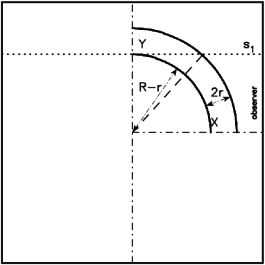
Fig. 11 : The section of one fourth of a torus is represented through a circle of radius $R$ and a bigger circle of radius $R+2r$. The observer is situated along the $x$ direction, the line of sight of maximum length is indicated.

7 The image from turbulence

The power released in the turbulent cascade has the same dimension of the emission coefficient and therefore can be considered the source of emissivity. We now consider a linear and a nonlinear relationship between turbulent power and emission coefficient.

7.1 Linear correspondence

It is assumed that the emission coefficient of the HH scales as the power released in turbulent kinetic energy, see equation (22),

$$\epsilon\sim\mathcal{P}\quad.$$ (84)

Due to the additive property of the optically thin medium along the line of sight, an integral operation is performed in order to obtain the intensity or brightness of emission

$$I(y)=\int_{0}^{\sqrt{{a}^{2}-{y}^{2}}}2\times\epsilon(r){dz}\quad,$$ (85)

with $r=\sqrt{z^{2}+y^{2}}$ and $a$ representing the jet radius, see Figure 8.

The intensity or brightness of emission according to formula (22) is

$$I(y)\sim\int_{0}^{\sqrt{{{\it a}}^{2}-{y}^{2}}}Il(z)dz$$ (86)

$$with\quad Il(z)=$$

$$\!4\,{\frac{\left({{\it z}}^{2}+{y}^{2}\right){A~{}}^{2}{{\it{b_{\frac{1}{2}}}}}^{8}{{\it a}}^{2}}{\left({{\it{b_{\frac{1}{2}}}}}^{2}+A~{}{{\it z}}^{2}+A~{}{y}^{2}\right)^{6}{x}^{2}\left(\sqrt{2}-1\right)\tan\left(\frac{\alpha}{2}\right)}}\quad.$$

This integral has an analytical solution but it is complicated and therefore Figure 12 only shows the numerical integration which presents a characteristic shape on the top of the blob called the ”valley on the top” .

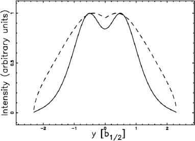
Fig. 12 : Intensity of radiation ${\it I(y)}$ in $b_{\frac{1}{2}}$ units across the turbulent jet when $z/d=50$ , $k$ =0.54, $A~{}$ = 0.414 and $\alpha_{deg}=2.0$ : full line ( linear correspondence) and dashed line (non linear correspondence,$f=4$) .

The maximum of this integral is at the point $y\approx 0.49{b_{\frac{1}{2}}}$ and the value of intensity or brightness at the maximum is $1.18$ times the value at the point $y=0$ ( the center of the jet). The near infrared images of HH 110 jet were interpreted as due to low velocity shocks produced by turbulent processes, see Noriega-Crespo et al. (1996). The spatial intensity or brightness distribution of $H_{2}$ , $H_{\alpha}$ and $[S_{II}]_{6717/31}$ perpendicular to the flow axis and along the cross section of knots in $HH110$ has a behavior that can be approximated by a Gaussian distribution , see Figure 4 in Noriega-Crespo et al. (1996). In one case , $H_{\alpha}$ in knot P of HH110 in Figure 5 in Noriega-Crespo et al. (1996) , it is possible to see a bump near the maximum of the intensity or brightness in the transversal direction. A second observation that presents a bimodal profile is the spatial $H_{\alpha}$ intensity distribution through the cross section of knot $I+J$ of HH110 visible in Figure 10 in Riera et al. (2003). A third observations is the $[SII]+[NII]$ profile in blob 1 of HH110 as in Figure 17 of Hartigan et al. (2009).

These three cases can be considered an observational evidence of the physical effect previously named ” valley on the top” .

Is also possible to build a 2D map of the surface brightness of emission computed according to the integral of equation(86) in a conical jet as HH1 and Figure 13 reports such a map.

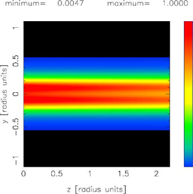
Fig. 13 : Theoretical 2D map of the surface brightness of emission corresponding to a $2.2~{}arcsec$ of HH1 around $z/d=110$. The parameters are $k$ =0.54, $A$ = 0.414 and $\alpha_{deg}=2.08$ . The integral operation is performed on a cubic grid of $400^{3}$ pixels.

In this case the values of emissivity are memorized on a 3D grid made by $(pixels)^{3}$ points. The integral is represented by a sum along the line of sight and Figure 14 reports a cut in the middle.

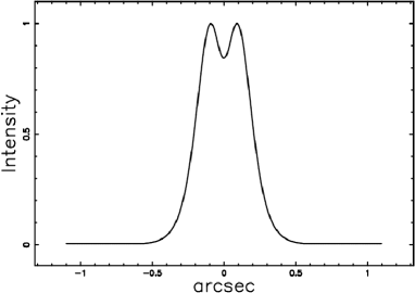
Fig. 14 : Intensity of HH1 represented through a cut in the y-direction , parameters as in Figure 13.

7.2 Non linear correspondence

From a careful inspection of formula (22) we see that the local power released in the turbulent cascade at $r=b_{\frac{1}{2}}$ scale as $\sim(\frac{1}{x})^{4}$ . In order to have a constant intensity or brightness along the jet we now consider the case

$$\epsilon\sim({\mathcal{P}})^{1/f}\quad,$$ (87)

which means that the intensity or brightness scales as

$$I(x)\sim d(x)(\frac{1}{x^{4}})^{1/f}\sim(\frac{1}{x})^{\frac{4}{f}-1}\quad.$$ (88)

The intensity or brightness of emission is

$$I(y)\sim\int_{0}^{\sqrt{{{\it a}}^{2}-{y}^{2}}}In(z)dz$$ (89)

$$with\quad In(z)=$$

$$(\!4\,{\frac{\left({{\it z}}^{2}+{y}^{2}\right){A~{}}^{2}{{\it{b_{\frac{1}{2}}}}}^{8}{{\it a}}^{2}}{\left({{\it{b_{\frac{1}{2}}}}}^{2}+A~{}{{\it z}}^{2}+A~{}{y}^{2}\right)^{6}{x}^{2}\left(\sqrt{2}-1\right)\tan\left(\frac{\alpha}{2}\right)}})^{\frac{1}{f}}.$$

The numerical result for $f=4$ , constant intensity or brightness along the main direction $x$, is reported in Figure 12 as a dashed line.

8 Conclusions

Law of motion The two theories here considered are based on the behavior of the centerline velocity , see the astrophysical equations (33) and (41) . From the two previous equations is possible to deduce the law of motion in presence of a stationary state, see the astrophysical equations (34) and (42) . On the way the flow rate of mass and the flow rate of energy (the mechanical luminosity) are also derived , see the astrophysical equations (37) ,(43) ,(40) , and (44).

Images The analysis of the intensity or brightness of a HH object has been split in three theoretical parts corresponding to three observable cases.

1. Transversal cut We have analyzed the case of constant number density , see equation (74), and the case of emissivity connected with the power released in the turbulent cascade, see equations (86) and (89). The intensity or brightness from turbulent cascade originates a curious effect at the center of the jet named ”valley on the top” .

2. Longitudinal cut Through a parametrization of the number density is possible to fit the theoretical and the observed intensity or brightness , see equation (79) .

3. 2D map The details of the HH’s image can be simulated imposing an arbitrary point of view of the observer. The enhancement in intensity or brightness is explored from a numerical point of view , see Figure (5) and (10). An analytical explanation of the enhancement in intensity or brightness is derived from the geometrical properties of the torus , see formula (82). Is interesting to underline that the ”torus effect” replaces the concept of bow shock. that is often used in order to explain the intensity enhancement along the HHs, see Krist et al. (1999); Smith, Khanzadyan, and Davis (2003).

References

- Anglada et al. (1992) Anglada, G., Rodriguez, L.F., Canto, J., Estalella, R., Torrelles, J.M.: ApJ 395, 494 (1992). doi:10.1086/171670
- Bally and Reipurth (2001) Bally, J., Reipurth, B.: ApJ 546, 299 (2001)
- Bally et al. (2006) Bally, J., Licht, D., Smith, N., Walawender, J.: AJ 131, 473 (2006). doi:10.1086/498265
- Beck et al. (2007) Beck, T.L., Riera, A., Raga, A.C., Reipurth, B.: AJ 133, 1221 (2007). doi:10.1086/511269
- Bicknell (1984) Bicknell, G.V.: ApJ 286, 68 (1984). doi:10.1086/162577
- Bird, Stewart, and Lightfoot (2002) Bird, R., Stewart, W., Lightfoot, E.: Transport phenomena ; second edition. John Wiley and Sons, New York (2002)
- Boehm, Noriega-Crespo, and Solf (1993) Boehm, K., Noriega-Crespo, A., Solf, J.: ApJ 416, 647 (1993). doi:10.1086/173265
- Boehm, Scott, and Solf (1991) Boehm, K.H., Scott, D.M., Solf, J.: ApJ 371, 248 (1991). doi:10.1086/169886
- Bohm, Raga, and Binette (1991) Bohm, K.H., Raga, A.C., Binette, L.: PASP 103, 85 (1991). doi:10.1086/132798
- Cabrit and Raga (2000) Cabrit, S., Raga, A.: A&A 354, 667 (2000)
- Cameron and Liseau (1990) Cameron, M., Liseau, R.: A&A 240, 409 (1990)
- Chrysostomou et al. (2000) Chrysostomou, A., Hobson, J., Davis, C.J., Smith, M.D., Berndsen, A.: MNRAS 314, 229 (2000)
- Ciardi et al. (2008) Ciardi, A., Ampleford, D.J., Lebedev, S.V., Stehle, C.: ApJ 678, 968 (2008). doi:10.1086/528679
- Curiel et al. (1989) Curiel, S., Rodriguez, L.F., Canto, J., Torrelles, J.M.: Revista Mexicana de Astronomia y Astrofisica 17, 137 (1989)
- Curiel et al. (1993) Curiel, S., Rodriguez, L.F., Moran, J.M., Canto, J.: ApJ 415, 191 (1993). doi:10.1086/173155
- Davis, Smith, and Eislöffel (2000) Davis, C.J., Smith, M.D., Eislöffel, J.: MNRAS 318, 747 (2000). doi:10.1046/j.1365-8711.2000.03766.x
- Davis et al. (2000) Davis, C.J., Berndsen, A., Smith, M.D., Chrysostomou, A., Hobson, J.: MNRAS 314, 241 (2000). doi:10.1046/j.1365-8711.2000.03305.x
- Davis et al. (2002) Davis, C.J., Stern, L., Ray, T.P., Chrysostomou, A.: A&A 382, 1021 (2002). doi:10.1051/0004-6361:20011680
- Dopita and Sutherland (2003) Dopita, M.A., Sutherland, R.S.: Astrophysics of the diffuse universe. Springer, Berlin (2003)
- Dopita, Binette, and Schwartz (1982) Dopita, M.A., Binette, L., Schwartz, R.D.: ApJ 261, 183 (1982). doi:10.1086/160329
- Favre, A. (1969) Favre, A.: Problems of hydrodynamics and continuum mechanics. Society for Industrial and Applied Mathematics, Philadelphia (1969)
- Ferrari, Trussoni, and Zaninetti (1979) Ferrari, A., Trussoni, E., Zaninetti, L.: A&A 79, 190 (1979)
- Ferrari, Trussoni, and Zaninetti (1981) Ferrari, A., Trussoni, E., Zaninetti, L.: MNRAS 196, 1051 (1981)
- Garcia Lopez et al. (2008) Garcia Lopez, R., Nisini, B., Giannini, T., Eislöffel, J., Bacciotti, F., Podio, L.: A&A 487, 1019 (2008). doi:10.1051/0004-6361:20079045
- Goldstein, Poole, and Safko (2002) Goldstein, H., Poole, C., Safko, J.: Classical mechanics. Addison-Wesley, San Francisco (2002)
- Gómez, Whitney, and Wood (1998) Gómez, M., Whitney, B.A., Wood, K.: AJ 115, 2018 (1998). doi:10.1086/300332
- Hardee, Clarke, and Howell (1995) Hardee, P.E., Clarke, D.A., Howell, D.A.: ApJ 441, 644 (1995). doi:10.1086/175389
- Haro (1952) Haro, G.: ApJ 115, 572 (1952). doi:10.1086/145576
- Hartigan (2008) Hartigan, P.: In: Bacciotti, F., Testi, L., Whelan, E. (eds.) Lecture Notes in Physics, Berlin Springer Verlag. Lecture Notes in Physics, Berlin Springer Verlag vol. 742, p. 15 (2008)
- Hartigan and Morse (2007) Hartigan, P., Morse, J.: ApJ 660, 426 (2007)
- Hartigan et al. (2009) Hartigan, P., Foster, J.M., Wilde, B.H., Coker, R.F., Rosen, P.A., Hansen, J.F., Blue, B.E., Williams, R.J.R., Carver, R., Frank, A.: ApJ 705, 1073 (2009). doi:10.1088/0004-637X/705/1/1073
- Helmholtz (1868) Helmholtz , H.: Monatsberichte der Kiglichen Preussiche Akademie der Wissenschaften zu Berlin 23, 215 (1868)
- Herbig (1950) Herbig, G.H.: ApJ 111, 11 (1950). doi:10.1086/145232
- Kelvin (1871) Kelvin, W.: Philosophical Magazine 42, 362 (1871)
- Krist et al. (1999) Krist, J.E., Stapelfeldt, K.R., Burrows, C.J., Hester, J.J., Watson, A.M., Ballester, G.E., Clarke, J.T., Crisp, D., Evans, R.W., Gallagher, J.S. III, Griffiths, R.E., Hoessel, J.G., Holtzman, J.A., Mould, J.R., Scowen, P.A., Trauger, J.T.: ApJ 515, 35 (1999). doi:10.1086/311961
- Landau (1987) Landau, L.: Fluid mechanics 2nd edition. Pergamon Press, New York (1987)
- Lang (1999) Lang, K.R.: Astrophysical formulae. (Third Edition). Springer, New York (1999)
- Li et al. (2007) Li, J.Z., Chu, Y.H., Gruendl, R.A., Bally, J., Su, W.: ApJ 659, 1373 (2007). doi:10.1086/504826
- Lightfoot and Glencross (1986) Lightfoot, J.F., Glencross, W.M.: MNRAS 221, 47 (1986)
- Lodders (2003) Lodders, K.: ApJ 591, 1220 (2003). doi:10.1086/375492
- Masciadri and Raga (2001) Masciadri, E., Raga, A.C.: A&A 376, 1073 (2001). doi:10.1051/0004-6361:20011052
- Masciadri et al. (2002) Masciadri, E., de Gouveia Dal Pino, E.M., Raga, A.C., Noriega-Crespo, A.: ApJ 580, 950 (2002)
- McCray and Layzer (1987) McCray, A. R. In: Dalgarno, Layzer, D. (eds.): Spectroscopy of astrophysical plasmas. Cambridge University Press, ??? (1987)
- Molinari and Noriega-Crespo (2002) Molinari, S., Noriega-Crespo, A.: AJ 123, 2010 (2002). doi:10.1086/339180
- Nisini et al. (2005) Nisini, B., Bacciotti, F., Giannini, T., Massi, F., Eislöffel, J., Podio, L., Ray, T.P.: A&A 441, 159 (2005). doi:10.1051/0004-6361:20053097
- Noriega-Crespo et al. (1996) Noriega-Crespo, A., Garnavich, P.M., Raga, A.C., Canto, J., Boehm, K.H.: ApJ 462, 804 (1996)
- Pope (2000) Pope, S.B.: Turbulent Flows. Cambridge University Press, Cambridge, UK (2000)
- Pravdo and Angelini (1993) Pravdo, S.H., Angelini, L.: ApJ 407, 232 (1993)
- Raga (1993) Raga, A.C.: Astrophysics and Space Science 208, 163 (1993)
- Raga, Noriega-Crespo, and Velázquez (2002) Raga, A.C., Noriega-Crespo, A., Velázquez, P.F.: ApJ 576, 149 (2002). doi:10.1086/343760
- Raga et al. (2009) Raga, A.C., Cantó, J., Rodríguez-González, A., Esquivel, A.: A&A 493, 115 (2009)
- Ray and Ershkovich (1983) Ray, T.P., Ershkovich, A.I.: MNRAS 204, 821 (1983)
- Reipurth and Aspin (1997) Reipurth, B., Aspin, C.: AJ 114, 2700 (1997)
- Reipurth and Raga (1999) Reipurth, B., Raga, A.C.: In: Lada, C.J., Kylafis, N.D. (eds.) NATO ASIC Proc. 540: The Origin of Stars and Planetary Systems, p. 267 (1999)
- Reipurth, Devine, and Bally (1998) Reipurth, B., Devine, D., Bally, J.: AJ 116, 1396 (1998). doi:10.1086/300513
- Reipurth et al. (2000) Reipurth, B., Heathcote, S., Yu, K.C., Bally, J., Rodríguez, L.F.: ApJ 534, 317 (2000). doi:10.1086/308757
- Reipurth et al. (2002) Reipurth, B., Heathcote, S., Morse, J., Hartigan, P., Bally, J.: AJ 123, 362 (2002). doi:10.1086/324738
- Riera et al. (2003) Riera, A., López, R., Raga, A.C., Estalella, R., Anglada, G.: A&A 400, 213 (2003). doi:10.1051/0004-6361:20021879
- Riera et al. (2005) Riera, A., Raga, A.C., Reipurth, B., Amram, P., Boulesteix, J., Toledano, O.: Revista Mexicana de Astronomia y Astrofisica 41, 371 (2005)
- Rodríguez and Reipurth (1989) Rodríguez, L.F., Reipurth, B.: Revista Mexicana de Astronomia y Astrofisica 17, 59 (1989)
- Rodriguez and Reipurth (1994) Rodriguez, L.F., Reipurth, B.: A&A 281, 882 (1994)
- Rolph, Scarrott, and Wolstencroft (1990) Rolph, C.D., Scarrott, S.M., Wolstencroft, R.D.: MNRAS 242, 109 (1990)
- Rybicki and Lightman (1991) Rybicki, G., Lightman, A.: Radiative processes in astrophysics. Wiley-Interscience, New-York (1991)
- Salas, Cruz-Gonzalez, and Porras (1998) Salas, L., Cruz-Gonzalez, I., Porras, A.: ApJ 500, 853 (1998). doi:10.1086/305743
- Scarrott et al. (1990) Scarrott, S.M., Gledhill, T.M., Rolph, C.D., Wolstencroft, R.D.: MNRAS 242, 419 (1990)
- Schlichting et al. (2004) Schlichting, H., Gersten, K., Krause, E., Oertel, H.J.: Boundary-Layer Theory . Springer, New-York (2004)
- Schwartz et al. (1988) Schwartz, R.D., Jennings, D.G., Williams, P.M., Cohen, M.: ApJ 334, 99 (1988). doi:10.1086/185321
- Smith, Khanzadyan, and Davis (2003) Smith, M.D., Khanzadyan, T., Davis, C.J.: MNRAS 339, 524 (2003). doi:10.1046/j.1365-8711.2003.06195.x
- Takami et al. (2005) Takami, M., Chrysostomou, A., Ray, T.P., Davis, C.J., Dent, W.R.F., Bailey, J., Tamura, M., Terada, H., Pyo, T.: Protostars and Planets V, 8207 (2005)
- Takami et al. (2006) Takami, M., Chrysostomou, A., Ray, T.P., Davis, C.J., Dent, W.R.F., Bailey, J., Tamura, M., Terada, H., Pyo, T.S.: ApJ 641, 357 (2006). doi:10.1086/500352
- Uchida et al. (1992) Uchida, Y., Todo, Y., Rosner, R., Shibata, K.: PASJ 44, 227 (1992)
- Zaninetti (1987) Zaninetti, L.: Physics of Fluids 30, 612 (1987)
- Zaninetti (1989) Zaninetti, L.: A&A 223, 369 (1989)
- Zaninetti (1999) Zaninetti, L.: Journal of Computational Physics 156, 382 (1999)
- Zaninetti (2007) Zaninetti, L.: Revista Mexicana de Astronomia y Astrofisica 43, 59 (2007)
- Zaninetti (2009) Zaninetti, L.: Revista Mexicana de Astronomia y Astrofisica 45, 25 (2009)