Stationary drag photocurrent caused by strong running wave in quantum wire: quantization of current.

Stationary drag photocurrent caused by strong effective running wave in quantum wire: quantization of current

Abstract

The stationary current induced by a strong running potential wave in one-dimensional system is studied. Such a wave can result from illumination of a straight quantum wire with special grating or spiral quantum wire by circular-polarized light. The wave drags electrons in the direction correlating with the direction of the system symmetry and polarization of light. In a pure system the wave induces minibands in the accompanied system of reference. We study the effect in the presence of impurity scattering. The current is an interplay between the wave drag and impurity braking. It was found that the drag current is quantized when the Fermi level gets into energy gaps.

Two main sources of the stationary photocurrent in homogeneous systems are known: light pressure (photon drag) grinb and photogalvanic belin , ivch ,we or ratchet effect. In the first case photons transmit their momenta to electrons and directly accelerate electrons, in the second case the light serves as an energy source, while the acceleration originates from a third body (impurities, phonons etc.), and the current direction correlates with the polarization of light via material tensors.

A related phenomenon is the electron drag by a surface acoustic wave (SAW) tal ,aiz ,aiz1 ,robin ,gov , ah ,ah1 ,kas . The wavelength of SAW is large as compared with electrons, so the periodicity is less important and electrons are treated as captured into dynamic quantum dots formed by potential minima. The discreteness of electrons leads to the SAW drag quantization. The quantization exists both with and without e-e interaction. If the wave amplitude is weak enough the quantum dots can not keep electrons and the picture fails.

In recent papers spiral ; we2 we have studied the electron drag by circular-polarized electromagnetic field in curved quantum wires, particularly, in quantum spirals. In such systems the electric field of a long external electromagnetic wave is converted to an effective short wave propagating along the wire. The wave drags electrons. The effect resembles the travelling-wave tube with the difference that the field remains almost uniform while the acting component of this field projected to the wire has a short wavelength. Besides, the effect takes place in a solid instead of vacuum.

We have considered the problem in the limit of weak field. It was also found that strong field bunches electrons in the potential minima, forcing them to move with the phase speed of the wave.

It should be emphasized that an effective wave can be produced in different ways, for example in the same way as in the travelling-wave tube, using metallic or dielectric spiral grating and straight quantum wire along the spiral axis. These inhomogeneous dielectric properties produce non-uniformity of local electric field and form the running wave. Such a construction permits to use not an exotic system like semiconductor spiral quantum wire prinz ; prinz1 , but more realistic systems: straight quantum wires together with spiral spacial field modulators. Another more simple design is a double grating like the one shown in Fig.1. This system also produces the running wave near the quantum wire. Other variants of running wave can be considered, e.g., plasmon wave.

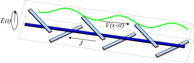
Figure 1: (Color online) Straight quantum wire with tilted metallic (isolator) grating in external alternating electric field ${\bf E}(t)$ circularly polarized in a plane orthogonal to the wire. The modulation of external field by the grating induces the running wave which drags electrons.

The purpose of the present paper is the study of the drag current in infinitely long homogeneous 1D system driven by the the potential wave whose wavelength is comparable with electronic. Such a wave changes the electron spectrum giving rise to the Bloch states. We have found that in these conditions the wave can drag electrons with the velocity of the wave. This phenomenon occurs when the Fermi level lies inside the forbidden band. That means quantization of current $J=e\omega N/\pi$, where $e$ is the electron charge, $\omega$ is the frequency of the wave and $N$ is the number of occupied bands. The accuracy of quantization is limited by the nonlinear response on the wave velocity. We shall demonstrate that the corrections to the quantized values are exponentially small if the wave velocity $s$ tends to zero.

Basic equations

Let us consider a strong potential wave $V=V_{0}\cos(kx-\omega t)$ propagating with velocity $s=\omega/k$ along the quantum wire in the presence of electron scattering. The scattering caused by impurities with the potential $U(x)=\sum_{j}u(x-x_{j})$ is assumed. If the field is strong one should include the wave field into the formation of electron states and consider the impurities as a perturbative factor. We shall use the coordinate system $x\to x-st$ accompanying the wave. In these coordinates the potential of the wave is stationary and the impurities are running back with the velocity $-s$: $U(x)\to U(x+st)$.

In the absence of impurities electron states $\psi_{\nu}(x),~{}~{}\nu\equiv(n,p)$ with a given quasimomentum $p$ in the $n$-th band obey the stationary Schrödinger equation:

$$\epsilon_{\nu}\psi_{\nu}(x)=-\frac{1}{2m}\frac{d^{2}}{dx^{2}}\psi_{\nu}(x)+V(x)\psi_{\nu}(x),$$ (1)

and the periodicity condition $\psi_{\nu}(x+\lambda)=e^{ip\lambda}\psi_{\nu}(x),$ where $\lambda=2\pi/k$ is the wavelength (we set $\hbar=1$). The states are represented by the Mathieu functions. With regard to the periodicity the Mathieu functions can be written as

$$\psi_{n,p}(x)=\frac{1}{\sqrt{L}}e^{ipx}\sum_{g}b^{n}_{p+g}e^{igx},$$

$g=kr$ is the vector of reciprocal lattice, $r$ is integer, $L$ is the length of the wire. The quantities $b^{n}_{p+g}$ are the Fourier harmonics of the Bloch amplitudes satisfying the equations

$$(2m\epsilon_{\nu}-(p+g)^{2})b^{n}_{p+g}-mV_{0}(b^{n}_{p+g+k}+b^{n}_{p+g-k})=0.$$ (2)

The quantities $b^{n}_{p+g}$ are real and orthonormalized by a condition $\sum_{g}b^{n^{\prime}}_{p+g}b^{n}_{p+g}=\delta_{nn^{\prime}}$.

The problem is studied in the framework of the kinetic equation approach. The stationary electron distribution function $f_{\nu}$ for electrons in the state $\nu$ obeys the kinetic equation $\hat{I}_{s}\{f_{\nu}\}=0$, where the collision operator $\hat{I}_{s}$ includes all scattering processes. The collision operator depends on the velocity $s$ as a parameter. If the velocity goes to zero the impurity potential becomes stationary and the distribution function converts to the equilibrium Fermi function $F_{\nu}\equiv F(\epsilon_{\nu})$. Hence, $\hat{I}_{0}\{F_{\nu}\}=0.$

We shall assume that the phase velocity $s$ is small. In this case $\hat{I}_{s}^{(1)}=\hat{I}_{s}-\hat{I}_{0}$ is small and one can expand the distribution function with respect to this smallness: $f_{\nu}=F_{\nu}+\chi_{\nu},$

$$\hat{I}_{0}\{\chi_{\nu}\}+\hat{I}^{(1)}\{F_{\nu}\}=0.$$ (3)

The Eq. (3) is the basic equation that determines the corrections to the distribution function. From this point we shall consider the impurities as a main factor of scattering. Thus, the collision operator can be prescribed to elastic processes caused by impurities. The impurity collision operator reads $\hat{I}_{s}\{f_{\nu}\}=\sum_{\nu^{\prime}}W_{\nu^{\prime},\nu}(f_{\nu^{\prime}}-f_{\nu})$

Additional simplification with the scattering operator $\hat{I}_{s}^{(1)}$ can be done by expanding it in powers of $s$. It should be emphasized that this expansion gives a finite result if the upper band is partially occupied (see below). The transitions between electron states caused by moving impurities decelerate electrons.

In the laboratory system the current is

$$j=en_{e}s+e\sum_{n}\int_{-k/2}^{k/2}\frac{dp}{\pi}v_{\nu}\chi_{\nu}^{(-)},~{}~{}~{}~{}v_{\nu}=\frac{d\epsilon_{\nu}}{dp},$$ (4)

where $\chi_{\nu}^{(-)}=(\chi_{\nu}-\chi_{\bar{\nu}})/2$, $\bar{\nu}\equiv(n,-p)$. The term $en_{e}s$ ($n_{e}$ being linear electron concentration) arises due to the transition from the moving frame of reference to the laboratory frame.

The collision term can be expressed via scattering probability on the moving impurities $W_{\nu,\nu^{\prime}}$. In the Born approximation the probability of scattering reads

$$W_{\nu^{\prime},\nu}=n_{i}\int dq|u(q)|^{2}|J_{\nu^{\prime},\nu}(q)|^{2}\delta(\epsilon_{\nu^{\prime}}-\epsilon_{\nu}+sq),$$ (5)

where $J_{\nu^{\prime};\nu}(q)=<\nu^{\prime}|e^{iqx}|\nu>$, $u(q)$ is the Fourier transform of the potential of individual impurity and $n_{i}$ is the linear density of impurities.

The expression for $\hat{I}_{0}\{\chi_{\nu}\}$ is algebraized

$$\hat{I}_{0}\{\chi_{\nu}\}=-\chi_{\nu}^{(-)}/\tau_{\nu},$$

where the relaxation time is

$$\tau_{\nu}^{-1}=\frac{n_{i}}{2}\int dq|u(q)|^{2}\sum_{p^{\prime}}|J_{\bar{\nu};\nu}(q)|^{2}\delta(\epsilon_{n,p^{\prime}}-\epsilon_{\nu}).$$

The summation over $p^{\prime}$ is limited by the first Brillouin zone $|p^{\prime}|<k/2$.

The quantity $\hat{I}_{s}\{F_{\nu}\}$ from Eq.(3) yeilds

$$\hat{I}_{s}\{F_{\nu}\}=n_{i}\int dq|u(q)|^{2}\times$$

$$\sum_{p^{\prime}}|J_{\nu^{\prime},\nu}(q)|^{2}\delta(\epsilon_{\nu^{\prime}}-\epsilon_{\nu}+qs)[F_{\nu^{\prime}}-F_{\nu}],$$ (6)

The matrix elements $J_{\nu^{\prime},\nu}(q)$ can be expressed via $b^{n}_{p}$:

$$J_{\nu^{\prime},\nu}=\sum_{g}\delta_{p^{\prime}-p-q,g}B_{\nu^{\prime},\nu}(g),~{}~{}~{}B_{\nu^{\prime},\nu}(g)=\sum_{g^{\prime}}b^{n^{\prime}}_{p^{\prime}+g^{\prime}}b^{n}_{p+g+g^{\prime}}.$$

Thus,

$$\chi_{\nu}^{(-)}=\tau_{\nu}n_{i}\int dq|u(q)|^{2}\sum_{\nu^{\prime}}|J_{\nu^{\prime},\nu}(q)|^{2}\times$$

$$\delta(\epsilon_{\nu^{\prime}}-\epsilon_{\nu}+qs)(F_{\nu^{\prime}}-F_{\nu}),$$ (7)

where $\tau_{\nu}^{-1}=2n_{i}|v_{\nu}|^{-1}\sum_{g}|u(2p+g)|^{2}|B_{\bar{\nu},\nu}(g)|^{2}.$

Metallic case

Expanding Eq.(Basic equations) by $s$ we find

$$\chi_{\nu}^{(-)}=-\frac{s\tau_{\nu}}{2}\sum_{g}\int_{-k/2}^{k/2}dp^{\prime}2\pi n_{i}|u(p^{\prime}-p-g)|^{2}$$

$$\times(p^{\prime}-p-g)|B_{\bar{\nu},\nu}(g)|^{2}\delta(\epsilon_{n,p^{\prime}}-\epsilon_{\nu})\frac{d}{d\epsilon}F(\epsilon_{\nu}).$$ (8)

It is seen from Eq.(Metallic case) that $\chi_{\nu}^{(-)}=0$ at zero temperature if the Fermi level lies outside the permitted band. If the Fermi level is inside the permitted band one can get to

$$j=\frac{e\omega}{\pi}\Big{(}N+((-1)^{N}-1)/2+(-1)^{N}\times$$

$$\frac{\sum_{g}(gd/2\pi)|u(2p_{0}+g)|^{2}|B_{N,-p_{0};N,p_{0}}(g)|^{2}}{\sum_{g}|u(2p_{0}+g)|^{2}|B_{N,-p_{0};N,p_{0}}(g)|^{2}})\Big{)},$$ (9)

where $N$, and $p_{0}>0$ satisfy the equation $\epsilon_{N}(p_{0})=\mu$; $N$ is the number of the last (partially) occupied permitted band, $p_{0}$ is the Fermi momentum. The first term in Eq.(Metallic case) originates from the first term in Eq.(4) and gives quantized values when $\mu$ goes outside the permitted bands.

The Equation (Metallic case) obtained in linear in $s$ approximation yields zero current in the accompanied system of reference if the Fermi level gets into forbidden bands. In this case the addition to the current, due to the transformation into the laboratory system gives $esn_{e}=e\omega N/\pi$, where $N$ is the number of the upper occupied band. Thus, the current becomes quantized.

Current (Metallic case) does not depend on the amplitude of a scattering potential. If the amplitude of the wave goes down the current tends to zero. This can be proved using the expression for $|B_{N,-p_{0};N,p_{0}}(g)|^{2}$ in the limit of empty lattice ($V_{0}=0$): $|B_{N,-p_{0};N,p_{0}}(g)|^{2}=\delta_{g,-Nk}$ if $N$ is even and $|B_{N,-p_{0};N,p_{0}}(g)|^{2}=\delta_{g,(N-1)k}$ if $N$ is odd.

We have calculated the current according to Eq.(Metallic case) for two types of impurity potential: short range ($u(q)=const$) and the Coulomb potential with $u(x)=1/\sqrt{x^{2}+\rho^{2}}$ and $u(q)=K_{0}(q\rho)$ ($\rho$ is the distance from impurities to the wire being assumed straight in this case, $K_{n}(x)$ is the modified Bessel function of the second kind).

The results are depicted in Figs. 2. The current exhibits quantized values in the forbidden bands and steep decrease in the permitted band near the bands edges. The direction of current everywhere is opposite to the wave. That reflects the drag of electrons induced by the wave. Mean value of current drops at $V_{0}\to 0$ or $\mu\to\infty$ due to the perturbative character of the drag, controlled by the parameter $(V_{0}/\mu)^{2}$. In fact, the dependence in minima corresponds to the classical model spiral . The large energy of electrons results in the weakness of the wave and quasiclassical behavior of states: in the higher permitted bands electrons almost do not ”feel” the wave.

This classical behavior is reproduced in the quantum case except for the vicinity of the narrow gaps, where the Bragg reflection occurs $\mu\approx\pi^{2}(2r+1)^{2}/2md^{2}$, $r=0,1,2...$. This reflection ”pins” electron to the wave, resulting in the quantized values of the current. In other words, full occupation of a band blocks transitions between this and empty band at low wave velocity. The transition between two regimes occurs in the energy distance of the gap order. That results in very steep slopes of the current dependence.

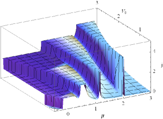
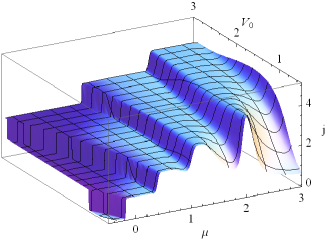
Figure 2: (Color online) Above: Drag current in units $e\omega/\pi$ versus the Fermi level $\mu$ and the wave amplitude $V_{0}$ in the case of short-range impurity potential $u(q)=\mbox{const}$. When $\mu$ gets into the forbidden bands, the current obtains integer values. Below: The same as in Fig.2 for $u(q)=K_{0}(q\rho)$ (Coulomb impurities).

The current approaches the quantized values from below when $\mu$ approaches the edges of permitted bands from their interior. This is explained by the character of the drag in the wave frame, namely, the drag of electrons near bottoms and the drag of holes near tops.

Insulator case

The previous consideration was based on the expansion with respect to the wave speed. This expansion yields exactly quantized values in the gaps. The corrections to the quantized values can be found from Eqs. (Basic equations) without expansion on the powers of $s$. This procedure results in the expression

$$j=\frac{e\omega N}{\pi}-en_{i}\int_{-k/2}^{k/2}\frac{dp}{\pi}\sum_{g;p^{\prime}}\sum_{n\leq N<n^{\prime}}^{\infty}\frac{l_{\nu}-l_{\nu^{\prime}}}{|v_{\nu^{\prime}}+s|}\times$$

$$|B_{\nu^{\prime},\nu}(g)|^{2}|u(p^{\prime}-p-g)|^{2}$$ (10)

Here $l_{\nu}=v_{\nu}\tau_{\nu}$; $p^{\prime}$ satisfies the equation $\epsilon_{\nu^{\prime}}+sp^{\prime}=\epsilon_{\nu}+(p+g)s$ (the summation over all roots is assumed).

The Pauli principle together with the conservation law permits transitions from occupied to empty bands only. At small $s$ the current in the insulating state is determined by the transitions between the last occupied and the first empty bands and $g\sim\Delta_{N}/s$, where $\Delta_{N}$ is a gap between these bands. The quantities $B_{N+1,p^{\prime};N,p}(g)$ rapidly decay with $g$ (and, hence, at $s\to 0$): $\log|B_{N+1,p^{\prime};N,p}(g)|\propto-\Delta_{N}/ks$. At the same time the other factors in Eq.(Insulator case) remain finite at $s\to 0$. Hence, at dielectric gaps the corrections to the quantized values are exponentially small.

.1 Discussion

It is desirable to compare the quantum case studied here to the classical drag effect considered earlier spiral . In the case of a strong classical wave, the current is simply $en_{e}s$. This value coincides with the quantum result if to express the current via the electron concentration. At the same time this dependence contains no steps.

The situation recalls the quantum Hall effect where the steps in the Hall current do not appear until the electron reservoir is taken into consideration. The question arises: do the impurity-induced local states in the energy gaps exist in the presence of a running wave? The answer is positive in the case of the slow wave if to replace the term ”local” by ”quasilocal”. At $s=0$ any impurity induces local states in the gaps. At $s\neq 0$ the potential becomes non-stationary and the transitions from the local to the free states appear. Nevertheless, similarly to transitions between free states considered earlier, at $s\to 0$ the transition amplitude and the widths of quasilocal states become exponentially small. The presence of tails of quasilocal states at the gap determines the reservoir and possibility of a continuous motion of the Fermi level in the energy gaps with electron density.

The current quantization is an allied problem to the charge quantization in adiabatic quantum pumps tau , brouw . In fact, the wave transmits exactly two electrons per cycle of field per an occupied band. The adiabaticity in the case considered here is provided by the low frequency. Nevertheless, the problems are different, since in the theory of the adiabatic quantum pumps, the discrete spectrum is supposed, while the system with a wave possesses a continuous spectrum.

It should be emphasized that the present approach differs from the studies of quantized SAW drag ah ,ah1 ,kas by the short length of wave resulting in the formation of the Bloch states instead of the local states in the wave minima and infinitely long quantum wire that demands taking the scattering into account. The difference from aiz1 ,robin is the absence of the e-e interaction. As a result of the spin degeneracy the steps in the current are observed at $e\omega N/\pi$ values instead of $e\omega N/2\pi$ and the current between steps (in metallic regime) goes through minima. The current quantization is explained by the Bragg scattering of electrons rather than the discreteness of electrons in the scenario of moving quantum dots utilized in the theory of the quantized SAW drag.

References

- (1) A. A. Grinberg, Zh. Eksp. Teor. Fiz. 58, 989 (1970) [Sov. Phys.-JETP 31, 531 (1970)].
- (2) V.I. Belinicher, B.I. Sturman, Sov. Phys. Usp. 23, 199 (1980) [Usp. Fiz. Nauk 130, 415 (1980)].
- (3) E.L. Ivchenko, G.E. Pikus, in Semiconductor Physics, V.M. Tushkevich and V.Ya. Frenkel, Eds., Cons. Bureau, p.427, New York (1986)
- (4) E.M. Baskin, M.D. Blokh, M.V. Entin, and L.I. Magarill, Phys.Stat.Sol.(b) 83, K97 (1977).
- (5) V.I. Talyanskii, J.M. Shilton, M. Pepper, C.G. Smith, C.J.B. Ford, E.H. Linfield, D.A. Ritchie, and G.A.C. Jones, Phys. Rev. B 56, 15180 (1997).
- (6) G.R.Aizin, G.Gumbs, M.Pepper, Phys. Rev. B, 58, 10589 (1998).
- (7) G.Gumbs, G.R.Aizin, M.Pepper, Phys. Rev. B, 60, R13954 (1999).
- (8) A. M. Robinson and C. H. W. Barnes, Phys. Rev. B, 63, 165418 (2001).
- (9) A.O.Govorov, A.V.Kalameitsev, V. M.Kovalev, H.-J.Kutschera, and A. Wixforth, Phys. Rev. Lett. 87, 226803 (2001).
- (10) A. Aharony and O. Entin-Wohlman, Phys. Rev. B, 65, 241401(R) (2002).
- (11) O. Entin-Wohlman, A. Aharony, Y. Levinson, Phys.Rev.B, 65, 195411 (2002).
- (12) V.Kashcheyeves, A.Aharony, O.Entin-Wohlman, European Physical Journal B, 39, 385 (2004).
- (13) L.I. Magarill, M.V. Entin, JETP Letters 78, 213 (2003) [Pis’ma ZhETF 78, 249 (2003)].
- (14) M.V. Entin, M.M. Mahmoodian, and L.I. Magarill, Physica E: Low-dimensional Systems and Nanostructures, doi:10.1016/j.physe.2009.10.028.
- (15) V.Ya.Prinz,V.A.Seleznev, A.K.Gutakovsky et al., Physica E: Low-dimensional Systems and Nanostructures, 6, 828 (2000).
- (16) V.Ya.Prinz, D.Grutzmacher, A.Beyer et al., Nanotechnology 12, S1 (2001).
- (17) D.J. Thouless, Phys. Rev. B, 27, 6083 (1983).
- (18) P.W. Brouwer Phys. Rev. B, 58, R10135 (1998).