QCD corrections to stoponium production at hadron colliders

Abstract

If the lighter top squark has no kinematically allowed two-body decays that conserve flavor, then it will live long enough to form hadronic bound states. The observation of the diphoton decays of stoponium could then provide a uniquely precise measurement of the top squark mass. In this paper, we calculate the cross section for the production of stoponium in a hadron collider at next-to-leading order (NLO) in QCD. We present numerical results for the cross section for production of stoponium at the LHC and study the dependence on beam energy, stoponium mass, and the renormalization and factorization scale. The cross-section is substantially increased by the NLO corrections, counteracting a corresponding decrease found earlier in the NLO diphoton branching ratio.

I Introduction

In low-energy supersymmetry, the usual collider signatures feature missing energy carried away by stable, neutral, weakly-interacting particles. Therefore, there are typically no kinematic mass peaks that could be used to precisely measure the individual superpartner masses. Other kinematic features can be used to determine mass differences with some precision, if the decay chains are favorable, but the overall mass scale of the sparticle spectrum is likely to be much more difficult to pin down accurately.

One exception to this may occur if new particles can form resonances that will decay by annihilation into only Standard Model particles with strong or electromagnetic interactions. A particularly interesting example is the possibility of stoponium, a ${}^{2S+1}{L}_{J}={}^{1}S_{0}$ bound state of the lighter top squark and top antisquark, which we will denote $\eta_{\tilde{t}}$. If the light top squark (or stop) $\tilde{t}_{1}$ has no kinematically allowed flavor-preserving two-body decays, then it will live long enough to form hadronic bound states including stoponium. Specifically, this will occur if the decays $\tilde{t}_{1}\rightarrow b\tilde{C}_{1}$ and $\tilde{t}_{1}\rightarrow t\tilde{N}_{1}$ are kinematically forbidden, where $\tilde{C}_{1}$ and $\tilde{N}_{1}$ are the lighter chargino and the lightest neutralino respectively. As pointed out originally by Drees and Nojiri Drees:1993yr ; Drees:1993uw , and re-examined recently in Martin:2008sv ; Martin:2009dj , decays of $s$-wave stoponium to $\gamma\gamma$ can provide a viable signal at the Large Hadron Collider (LHC) with sufficient beam energy and integrated luminosity. The signal will appear as a peak with width determined by detector resolution on top of a smoothly falling background. This could provide a uniquely precise measurement of the top squark mass, which would in turn serve as a “standard candle” for kinematics of the supersymmetric sector. (See also refs. Nappi:1981ft -Kats:2009bv for other work related to stoponium at colliders.)

As reviewed in more detail in refs. Martin:2008sv ; Martin:2009dj , there are at least two good motivations for considering top squarks light enough to form bound states. First, in models of “compressed supersymmetry” compressed , the top squark automatically comes out relatively light (compared to so-called mSUGRA models). These models can provide the right amount of dark matter provided that the mass difference between $\tilde{t}_{1}$ and $\tilde{N}_{1}$ is less than the top quark mass, with $m_{\tilde{t}_{1}}$ between about 200 GeV and 400 GeV. Second, minimal supersymmetric models that can provide baryogenesis at the electroweak scale EWbaryogenesis ; EWbaryogenesisnew require a quasi-stable stop with a mass that is currently estimated to be in the range from approximately 118 GeV to 135 GeV.

The production and decay of stoponium as studied in refs. Drees:1993yr ; Drees:1993uw ; Martin:2008sv at leading order (LO) are subject to large QCD radiative corrections and a strong dependence on the renormalization scale. The purpose of the present paper is to compute the corrections to stoponium production in hadronic collisions at next-to-leading order (NLO) in QCD, in order to help interpret limits on, or discovery of, a stoponium resonance at the LHC. This result will complement (and will make use of) our previous calculation of the QCD NLO corrections to stoponium decay Martin:2009dj .

In this paper, we will model the inclusive production of stoponium at a hadron collider as factored into the production of the free squark-antisquark pair with the same momentum in a color-singlet state and the binding of the pair into the stoponium bound state. For each pair of initial-state partons, the production amplitude for the squark-antisquark state with quantum numbers identical to the scalar ground state of stoponium is calculated in perturbative QCD, then related to the parton-level stoponium production cross section by integrating over the phase space that models the non-perturbative process of bound state formation using the wavefunction at the origin. In carrying out this program, we will closely follow the methods of ref. Kuhn:1992qw , which treated the analogous case of ${}^{1}S_{0}$ toponium ($\eta_{t}$) production. (Ref. Kuhn:1992qw was written before the mass of the top quark was known to be too large to allow it to form bound states, so toponium was a viable possibility at that time.)

It is well known that the “static color singlet model” just described has failed spectacularly in explaining the observed $J/\psi$ and $\psi(2S)$ prompt production in hadronic collisions. The color singlet model prediction for the prompt production cross section of the $\psi(2S)$ charmonium state is too small by a factor of about 50, while the prediction for prompt $J/\psi$ is too small by a factor of about 6, compared to the Tevatron data Abe:1997jz . (The $\Upsilon$ production cross section data UpsilonCDF ; UpsilonDzero seems to be acceptably fit by the color singlet model after inclusion of NNLO contributions UpsilonNNLO .) The failure of the static color singlet model in the charmonium case is due in part to the assumption that the hadronization of $Q\overline{Q}$ can be factored into perturbative calculations of the production of open $Q\overline{Q}$ with color and spin identical to the bound state and the nonrelativistic probability for annihilation at the origin. The discrepancy has provoked a variety of efforts to go beyond the static color singlet model in calculations; for reviews see Petrelli:1997ge -Lansberg:2008gk . For example, more general analyses performed using the NRQCD effective theory for nonrelativistic heavy quarks show that large enhancements to quarkonium production can come from the production of the constituent quarks in several different color and angular momentum states that can transition to the desired bound state. In this approach, the parton-level differential cross section for the production of a bound state $\Phi$ in a collider is given by:

$$d\hat{\sigma}(ab\rightarrow\Phi+X)=\sum_{n}d\hat{\sigma}(ab\rightarrow Q\overline{Q}[n]+X)\langle\mathcal{O}^{\Phi}[n]\rangle,$$ (1.1)

Here the differential cross section is factored into the short-distance perturbatively calculated cross sections initiated by partons $a,b$ for the production of a quark-antiquark pair $Q\overline{Q}$ in the color and spin state $n$, and the long-distance transition probabilities $\langle\mathcal{O}^{\Phi}[n]\rangle$ that describe the nonperturbative component of the hadronization. The sum over states $n$ can be thought of as a perturbative series in the relative velocity $v$, which separates the long- and short-distance scales. So-called power counting rules are used to determine the relative order of each transition based on the effective theory interactions it represents Lepage:1992tx ; Bodwin:1994jh . The series converges more quickly as the mass of the quarks increases; for charmonium $v$ is approximately 0.3 and for bottomonium $v\sim 0.1$. Transitions suppressed by the relative velocity can nevertheless have large cross sections and be much larger than the direct production assumed in the color singlet model, which may help explain the large observed prompt production cross sections. However, measurements of the $J/\psi$ polarization Psipolarization at the Tevatron and other measurements PHENIX by PHENIX at RHIC do not seem to fit well the predictions of the NRQCD approach.

Fortunately, however, the importance of corrections beyond the static color-singlet model should be relatively much less important for stoponium production, for several reasons. First, because the top squarks are much heavier, expansions in $\alpha_{S}$ should converge more quickly. Second, because $\eta_{\tilde{t}}$ formed from scalars is a $J=0$ state, the LO cross section for the color singlet state does not require an extra gluon, as is the case for $J/\psi$, $\psi(2S)$ or $\Upsilon$ production at leading order. Finally, in the stoponium case, all color octet states that can transition to the color singlet stoponium state ${}^{1}S_{0}$ are of relative order $v^{4}$. They are already negligible in the case of $\eta_{b}$ production at next-to-leading order Maltoni:2004hv , and since $v$ scales with $\alpha_{S}$, these color-octet transitions should be suppressed by an additional large factor for stoponium. These considerations justify our use of the color singlet model to calculate the radiative corrections to scalar stoponium production and decay in perturbative QCD. Note that this essentially amounts to letting the wavefunction(s) at the origin $R(0)$ in a potential model play the role of the spin-0 color-singlet matrix element(s) in eq. (1.1), while neglecting the effects of the higher spin or color matrix elements. A more accurate treatment including those effects may eventually be necessary, but is beyond the scope of the present paper and in any case would require some way of estimating the other relevant matrix elements, which are presently unavailable.

The organization of the remainder of this paper is as follows. In section II we provide the NLO parton-level cross sections for stoponium production in hadronic collisions in the static color singlet model. In section III we discuss how to turn these calculations into hadron-collision cross sections. In section IV, we provide numerical results for the NLO stoponium production cross section in proton-proton collisions, studying the dependence on beam energies relevant for the CERN Large Hadron Collider (LHC), on the stoponium mass, and on the renormalization and factorization scale. We also review the next-to-leading order hadronic and diphoton branching ratios for the annihilation decays found in Martin:2009dj , which we use to estimate the NLO QCD cross section times branching ratio for the observable signal $pp\rightarrow\eta_{\tilde{t}}+X\rightarrow\gamma\gamma+X$ in scenarios where the hadronic partial width dominates the full width, and discuss corrections that apply to this idealized result in compressed supersymmetry and in models with electroweak-scale baryogenesis.

II Parton-level cross sections

In this section, we calculate the individual parton-level cross sections that contribute to the hadronic production of stoponium in NLO QCD. We will closely follow the method used by Kühn and Mirkes to calculate radiative corrections to toponium production in ref. Kuhn:1992qw . Although the virtual corrections to the leading-order diagrams for stoponium differ from the toponium result, we will show that the other radiative corrections contributing to the next-to-leading order cross section have the same form for stoponium as for their toponium counterparts, when both are written in terms of their corresponding leading order results. The relevant Feynman rules for our calculation can be found in Martin:2009dj . Both ultraviolet and infrared divergences will be dealt with by dimensional regularization.

In order to compute the parton-level cross-sections for stoponium production from the rate for open squark-antisquark production, integration over the final-state phase space must be restricted to the subspace containing the bound state. Let $d{\mathcal{P}}_{N}(k_{1},k_{2};p_{1},p_{2},\ldots,p_{N})$ be the Lorentz-invariant differential phase space element for an $N$-body final state. In our case, $N=2$ or 3, and $k_{1}$ and $k_{2}$ will be the initial (massless) parton momenta and $p_{1}$ and $p_{2}$ are the final squark and antisquark momenta and $p_{3}$ is a possible final state (massless) parton momentum. To project onto the bound state phase space, we require the final-state squarks to have identical 4-momenta, letting $p=p_{1}=p_{2}$, so that $2p$ is the stoponium momentum, and use the radial wavefunction at the origin $R(0)$ (normalized so that $\psi(\vec{r})=R(r)/\sqrt{4\pi}$ for an $S$-wave state) to characterize the long-range behavior of the squark hadronization. As a consequence of this projection, the relevant 2-body and 3-body differential phase space factors in $d=4-2\epsilon$ dimensions are replaced by

$$d\mathcal{P}_{2} \rightarrow \frac{|R(0)|^{2}}{M}\delta(\hat{s}-M^{2}),$$ (2.1)

$$d\mathcal{P}_{3} \rightarrow \frac{|R(0)|^{2}}{16\pi^{2}\Gamma(1-\epsilon)M}\left(\frac{4\pi\hat{s}}{\hat{u}\hat{t}}\right)^{\epsilon}\frac{d\hat{t}}{\hat{s}},$$ (2.2)

where the parton-level Mandelstam variables are defined by

$$\hat{s}=(k_{1}+k_{2})^{2},\qquad\hat{t}=(2p-k_{1})^{2},\qquad\hat{u}=(2p-k_{2})^{2},$$ (2.3)

and satisfy

$$\hat{s}+\hat{t}+\hat{u}=4p^{2}=M^{2}$$ (2.4)

where $M=2m_{\tilde{t}}-E_{\rm binding}\approx 2m_{\tilde{t}}$ is the bound state mass. Here and in the remainder of the paper, we will often write $\tilde{t}$ without the subscript 1 and $M$ instead of $M_{\eta_{\tilde{t}}}$, for simplicity.

II.1 Gluon fusion at leading order

Figure 1: The leading-order diagrams for the production of stoponium.

The parton-level diagrams for the leading order production of stoponium are in Fig. 1. In this calculation, the squark and antisquark are restricted to color combinations appropriate for the singlet bound state using a wavefunction projection factor $\delta_{i}^{j}/\sqrt{N_{c}}$, where $i,j$ are $SU(N_{c})$ fundamental representation indices (with $N_{c}=3$ in the real world). The squared amplitude obtained from these diagrams, averaged over initial color and polarization and summed over final color, is

$$\frac{1}{(d-2)^{2}(N_{c}^{2}-1)^{2}}\sum{|\mathcal{M}|^{2}}=\frac{8\pi^{2}\widehat{\alpha}_{S}^{2}\mu^{4\epsilon}}{N_{c}(N_{c}^{2}-1)(1-\epsilon)},$$ (2.5)

where $\mu$ is the regularization scale and $\widehat{\alpha}_{S}$ is the bare coupling.

The leading order differential cross section for stop-antistop production in a color singlet state is therefore

$$d\hat{\sigma}_{\rm LO}(gg\rightarrow\tilde{t}\tilde{t}^{*})=\frac{1}{2\hat{s}}\frac{1}{(d-2)^{2}(N_{c}^{2}-1)^{2}}\sum{|\mathcal{M}|^{2}}d\mathcal{P}_{2},$$ (2.6)

where $\hat{s}$ is the parton-level center-of-momentum energy squared. The leading-order cross-section for scalar stoponium production is obtained from this by the projection that restricts the squark and antisquark to identical 4-momenta and includes the probability of annihilation at the origin, using eq. (2.1):

$$\hat{\sigma}_{\rm LO}(gg\rightarrow\eta_{\tilde{t}})=\frac{4\pi^{2}\widehat{\alpha}_{S}^{2}\mu^{4\epsilon}}{N_{c}(N_{c}^{2}-1)(1-\epsilon)}\frac{|R(0)|^{2}}{M^{3}}\frac{\delta(1-z)}{\hat{s}},$$ (2.7)

where

$$z\equiv M^{2}/\hat{s}.$$ (2.8)

Note that the result (2.7) for LO stoponium production is a factor of $2(1-2\epsilon)$ smaller than the corresponding result for toponium obtained in eq. (10) of ref. Kuhn:1992qw .

II.2 Gluon fusion at NLO

The corrections to leading-order gluon fusion can be divided into two parts - the virtual corrections coming from gluon loops in the leading-order diagrams and the corrections that involve the real emission of an additional gluon in the final state. The virtual corrections to stoponium production through gluon fusion are identical to the virtual corrections to stoponium annihilation to two gluons, which we have already calculated Martin:2009dj . Adding up the two-particle cuts in Tables I and II of ref. Martin:2009dj , and combining with eq. (2.7), we find

$${\hat{\sigma}}_{\mathrm{LO+virtual}}(gg\rightarrow\eta_{\tilde{t}}) = \sigma_{0}\delta(1-z)\frac{\mu^{4\epsilon}}{1-\epsilon}\Bigg{\{}1+\frac{\alpha_{S}}{\pi}\left(\frac{4\pi\mu^{2}}{M^{2}}\right)^{\epsilon}\Gamma(1+\epsilon)\Big{[}\frac{b_{0}}{2}\ln\left(\frac{Q^{2}}{M^{2}}\right)$$ (2.9)

$$-\frac{N_{c}}{\epsilon^{2}_{\rm IR}}-\frac{b_{0}}{2\epsilon_{\rm IR}}+\left(1+\frac{5\pi^{2}}{12}\right)N_{c}-\left(3+\frac{\pi^{2}}{4}\right)C_{F}\Big{]}\Bigg{\}},$$

where $C_{F}=(N_{c}^{2}-1)/2N_{c}$, and

$$b_{0} = \frac{11}{3}N_{c}-\frac{2}{3}n_{f},$$ (2.10)

with $n_{f}$ the number of quark flavors, and we define for future convenience

$$\sigma_{0}\equiv\frac{4\pi^{2}\alpha_{S}^{2}}{N_{c}(N_{c}^{2}-1)\hat{s}}\frac{|R(0)|^{2}}{M^{3}}.$$ (2.11)

In eqs. (2.9) and (2.11), $\alpha_{S}(Q)$ is the $\overline{\rm MS}$ coupling renormalized at the scale $Q$, related at one-loop order to the bare coupling $\widehat{\alpha}_{S}$ and the regularization scale $\mu$ by

$$\widehat{\alpha}_{S}=\alpha_{S}\left[1-\frac{\alpha_{S}}{\pi}\frac{b_{0}}{4}\left(\frac{1}{\epsilon_{\rm UV}}+\ln(4\pi\mu^{2}/Q^{2})-\gamma_{E}\right)\right].$$ (2.12)

Note that we do not include the two-cut diagrams relating to the insertion of squark loops in the gluon propagator (diagrams q1-q4 of ref. Martin:2009dj ) since we will use $\alpha_{S}^{(n_{f})}$ from the $n_{f}=5$-quark effective theory to be consistent with the parton distribution functions we will use. We have also made the replacement $\ln(m_{f}^{2}/M^{2})\rightarrow 1/\epsilon_{\rm IR}$ in the mass singularity arising from quark loops and the $1/v$ singularity is absorbed into the definition of the bound state wavefunction.

The squared matrix element for real gluon emission can be obtained from that of the diagrams for $ggg\rightarrow\tilde{t}\tilde{t}^{*}$ in Figure 2 by crossing one gluon to the final state in all possible ways.

Figure 2: Non-zero diagrams related by crossing symmetry to the real gluon emission corrections to scalar stoponium production. Diagrams related to (a) and (b) by arrow reversal are also included with them but not shown.

The three external gluons carry labels $i,j,n=1,2,3$ and carry momenta and polarizations $k_{i}$ and $\epsilon_{i}$, etc. The stop and antistop each with mass $m$ have the same momentum $p$ (since we let the relative velocity go to zero). The matrix element resulting from Figure 2 is

$$\mathcal{M}_{(i,j,n)}=\frac{g^{3}f^{a_{i}a_{j}a_{n}}}{\sqrt{N_{c}}}\epsilon_{i}^{\mu}\epsilon_{j}^{\nu}\epsilon_{n}^{\rho}\left[\mathcal{M}^{(a)}_{\mu\nu\rho}+\mathcal{M}^{(b)}_{\mu\nu\rho}+\mathcal{M}^{(c)}_{\mu\nu\rho}\right],$$ (2.13)

where

$$i\mathcal{M}^{(a)}_{\mu\nu\rho} = \frac{(k_{j}+k_{n})_{\mu}(k_{n}-k_{i})_{\nu}(k_{i}+k_{j})_{\rho}}{2[(p-k_{i})^{2}-m^{2}][(p-k_{n})^{2}-m^{2}]},$$ (2.14)

$$i\mathcal{M}^{(b)}_{\mu\nu\rho} = \frac{[g_{\mu\nu}(k_{i}-k_{j})\cdot k_{n}+(k_{i}+2k_{j})_{\mu}(k_{n})_{\nu}-(2k_{i}+k_{j})_{\nu}(k_{n})_{\mu}](k_{i}+k_{j})_{\rho}}{[(p-k_{n})^{2}-m^{2}](k_{i}+k_{j})^{2}},$$ (2.15)

$$i\mathcal{M}^{(c)}_{\mu\nu\rho} = [g_{\mu\nu}(k_{i}-k_{j})_{\rho}+g_{\nu\rho}(k_{i}+2k_{j})_{\mu}-g_{\rho\mu}(2k_{i}+k_{j})_{\nu}]/(k_{i}+k_{j})^{2}$$ (2.16)

correspond to the contributions from diagrams of types 2(a), (b), and (c) respectively. The total matrix element that includes all diagrams is

$$\mathcal{M}=\sum_{(i,j,n)}\mathcal{M}_{(i,j,n)},$$ (2.17)

where $\sum_{(i,j,n)}$ represents a sum over the six permutations $(i,j,n)=(1,2,3)$, $(1,3,2)$, $(2,1,3)$, $(2,3,1)$, $(3,1,2)$, $(3,2,1)$. Taking the labels 1,2 to refer to the initial-state gluons and 3 for the final-state gluon, the spin-summed squared matrix element for $gg\rightarrow\tilde{t}\tilde{t}^{*}g$ is equal to $\sum|\mathcal{M}|^{2}$ by crossing, when expressed in terms of the parton-level Mandelstam variables defined in eq. (2.3).

The sums over the physical polarizations of the gluons are performed using

$$\sum_{\lambda}\epsilon_{\mu}(\lambda,k)\epsilon_{\nu}^{*}(\lambda,k)=-g_{\mu\nu}+\frac{n_{\mu}k_{\nu}+n_{\nu}k_{\mu}}{n\cdot k}-\frac{n^{2}k_{\mu}k_{\nu}}{(n\cdot k)^{2}}$$ (2.18)

where $k$ is the momentum of the gluon in question and $n$ is an arbitrary 4-vector. This avoids the added complication of needing to cancel unphysical polarizations using additional diagrams that include ghost loops for each triple gluon vertex. Note that it is convenient for any given gluon polarization sum to choose any other of the massless gluon momenta for $n$. Including factors for the averaging over initial gluon polarization and color, this parton-level differential cross section is

$$d\hat{\sigma}(gg\rightarrow\eta_{\tilde{t}}g)=\frac{1}{2\hat{s}}\frac{1}{(d-2)^{2}(N_{c}^{2}-1)^{2}}\sum|\mathcal{M}|^{2}\ d\mathcal{P}_{3},$$ (2.19)

where $d\mathcal{P}_{3}$ is understood to be replaced according to eq. (2.2) to obtain the stoponium + X differential phase space. The result is

$$d\hat{\sigma}(gg\rightarrow\eta_{\tilde{t}}g) = \sigma_{0}\frac{\alpha_{S}}{2\pi}N_{c}\frac{M^{2}}{\hat{s}}\left(\frac{4\pi\mu^{2}\hat{s}}{\hat{u}\hat{t}}\right)^{\epsilon}\frac{\mu^{4\epsilon}}{\Gamma(2-\epsilon)}\Bigg{[}\frac{\hat{s}\hat{t}+\hat{t}\hat{u}+\hat{u}\hat{s}}{(\hat{s}-M^{2})(\hat{t}-M^{2})(\hat{u}-M^{2})}\Bigg{]}^{2}$$ (2.20)

$$\Bigg{[}\frac{M^{8}+\hat{s}^{4}+\hat{t}^{4}+\hat{u}^{4}}{\hat{s}\hat{t}\hat{u}}\Bigg{]}\ d\hat{t},$$

where we have dropped a term proportional to $\epsilon$ that does not have a potentially singular denominator after angular integration in the $\epsilon\rightarrow 0$ limit.

Angular integration is carried out by replacing the Mandelstam variables with the dimensionless variables $y$ and $z$ defined on the interval $[0,1]$ by eq. (2.8) and

$$y=(1+\cos\theta)/2,$$ (2.21)

where $\theta$ is the angle in the center-of-momentum frame between the initial-state parton with momentum $k_{1}$ and the stoponium momentum direction. This implies that

$$\hat{t}=-M^{2}(1-y)(1-z)/z,\qquad\qquad\hat{u}=-M^{2}y(1-z)/z.$$ (2.22)

In terms of $y$ and $z$, the partonic cross section is

$$\hat{\sigma}(gg\rightarrow\eta_{\tilde{t}}g) = \sigma_{0}\frac{\alpha_{S}}{\pi}N_{c}\left(\frac{4\pi\mu^{2}}{M^{2}}\right)^{\epsilon}\frac{\mu^{4\epsilon}}{\Gamma(2-\epsilon)}z^{1+\epsilon}(1-z)^{-1-2\epsilon}\int_{0}^{1}dy\,y^{-\epsilon}(1-y)^{-1-\epsilon}$$ (2.23)

$$\left(\frac{1-y(1-y)(1-z)}{[1-y(1-z)][z+y(1-z)]}\right)^{2}\left(z^{4}+1+(1-z)^{4}\left[(1-y)^{4}+y^{4}\right]\right),$$

where we have used the symmetry of the rest of the integrand under $y\rightarrow 1-y$ to replace $y^{-1-\epsilon}(1-y)^{-1-\epsilon}$ with $2y^{-\epsilon}(1-y)^{-1-\epsilon}$.

To compute this integral, one uses plus distributions to simplify the integrand and isolate the soft and collinear divergences before integration is carried out. The plus distribution $\left(F(x)\right)_{+}$ of a function $F(x)$ is defined by Field:1989uq

$$\left(F(x)\right)_{+}\equiv\lim_{\beta\rightarrow 0}\Bigg{[}F(x)\Theta(1-x-\beta)-\delta(1-x-\beta)\int_{0}^{1-\beta}F(y)\,dy\Bigg{]},$$ (2.24)

from which follows the identity

$$\int_{0}^{1}G(x)\left(F(x)\right){{}_{+}}\,dx=\int_{0}^{1}\Big{[}G(x)-G(1)\Big{]}F(x)\,dx$$ (2.25)

and the expansion identities

$$y^{-\epsilon}(1-y)^{-1-\epsilon}=-\frac{1}{\epsilon}\delta(1-y)+\left(\frac{1}{1-y}\right)_{+}-\epsilon\ \frac{\ln y}{1-y}-\epsilon\ \left(\frac{\ln(1-y)}{1-y}\right)_{+},$$ (2.26)

$$z^{\epsilon}(1-z)^{-1-2\epsilon}=-\frac{1}{2\epsilon}\delta(1-z)+\left(\frac{1}{1-z}\right)_{+}+\epsilon\ \frac{\ln z}{1-z}-2\epsilon\ \left(\frac{\ln(1-z)}{1-z}\right)_{+}.$$ (2.27)

Using these expansions in eq. (2.23) and integrating over $y$ using eq. (2.25), one obtains:

$$\hat{\sigma}(gg\rightarrow\eta_{\tilde{t}}g) = \sigma_{0}\frac{\alpha_{S}}{\pi}2N_{c}\left(\frac{4\pi\mu^{2}}{M^{2}}\right)^{\epsilon}\frac{\mu^{4\epsilon}\Gamma(1+\epsilon)}{1-\epsilon}\Bigg{\{}\frac{1}{2\epsilon^{2}}\delta(1-z)-\frac{\pi^{2}}{6}\delta(1-z)$$ (2.28)

$$-\frac{1}{\epsilon}\frac{[1-z(1-z)]^{2}}{z}\left(\frac{1}{1-z}\right)_{+}-\Big{[}\frac{11z^{6}+2z^{4}+24z^{3}+23z^{2}+12}{12z(1+z)^{2}}$$

$$+\frac{2z^{7}+3z^{6}+z^{4}+2z^{3}+5z^{2}-1}{z(1-z)(1+z)^{3}}\ln z\Big{]}\left(\frac{1}{1-z}\right)_{+}$$

$$+\frac{[1-z(1-z)]^{2}}{z(1-z)}\Big{[}2(1-z)\left(\frac{\ln(1-z)}{1-z}\right)_{+}-\ln z\Big{]}\Bigg{\}}.$$

Further simplification can be carried out by noting that if $G(1)=0$, then eq. (2.25) implies

$$\int_{0}^{1}G(z)\left(F(z)\right)_{+}\,dz=\int_{0}^{1}G(z)F(z)\,dx,$$ (2.29)

and therefore one can simply replace the plus distributions multiplying such functions accordingly, under the assumption that we will eventually integrate to an upper limit $z=1$. The result of this simplification is

$$\hat{\sigma}(gg\rightarrow\eta_{\tilde{t}}g) = \sigma_{0}\frac{\alpha_{S}}{\pi}N_{c}\left(\frac{4\pi\mu^{2}}{M^{2}}\right)^{\epsilon}\frac{\mu^{4\epsilon}\Gamma(1+\epsilon)}{1-\epsilon}\Bigg{\{}\frac{1}{\epsilon^{2}}\delta(1-z)-\frac{\pi^{2}}{3}\delta(1-z)$$ (2.30)

$$-\frac{2}{\epsilon}\Big{[}\frac{1}{z}+\left(\frac{1}{1-z}\right)_{+}+z(1-z)-2\Big{]}+F_{gg}(z)\Bigg{\}},$$

where

$$F_{gg}(z) = \frac{11z^{5}+11z^{4}+13z^{3}+19z^{2}+6z-12}{6z(1+z)^{2}}+4\left(\frac{1}{z}+z(1-z)-2\right)\ln(1-z)$$ (2.31)

$$+4\left(\frac{\ln(1-z)}{1-z}\right)_{+}+\frac{2(z^{3}-2z^{2}-3z-2)(z^{3}-z+2)z\ln z}{(1+z)^{3}(1-z)^{2}}-\frac{3}{1-z}.$$

This is identical in form to the corresponding real emission correction to the leading order parton-level toponium cross section Kuhn:1992qw , when both are written in terms of their respective LO results $\sigma_{0}$.

To get the full next-to-leading order QCD cross section for gluon fusion, one must add the leading order plus virtual corrections from eq. (2.9) and real emission corrections from (2.30), resulting in

$$\hat{\sigma}(gg\rightarrow\eta_{\tilde{t}}+X) = \sigma_{0}\frac{\mu^{4\epsilon}}{1-\epsilon}\Bigg{\{}\delta(1-z)+\frac{\alpha_{S}}{\pi}\Gamma(1+\epsilon)\left(\frac{4\pi\mu^{2}}{M^{2}}\right)^{\epsilon}\Bigg{[}\delta(1-z)\bigg{\{}\frac{b_{0}}{2}\ln\left(\frac{Q^{2}}{M^{2}}\right)$$ (2.32)

$$+(N_{c}-3C_{F})\left(1+\frac{\pi^{2}}{12}\right)\bigg{\}}+N_{c}F_{gg}(z)-\frac{1}{\epsilon_{\rm IR}}P_{gg}(z)\Bigg{]}\Bigg{\}},$$

where

$$P_{gg}(z)=2N_{c}\left[\frac{1}{z}+\left(\frac{1}{1-z}\right)_{+}+z(1-z)-2\right]+\frac{b_{0}}{2}\delta(1-z).$$ (2.33)

Factorization requires the subtraction of

$$\sigma_{0}\frac{\alpha_{S}}{\pi}\frac{\mu^{4\epsilon}\Gamma(1+\epsilon)}{1-\epsilon}\left(\frac{4\pi\mu^{2}}{Q_{F}^{2}}\right)^{\epsilon}\left(-\frac{1}{\epsilon_{\rm IR}}P_{gg}(z)+C_{gg}(z)\right)$$ (2.34)

from eq. (2.32), where $C_{gg}(z)$ is scheme-dependent. In the $\overline{\rm MS}$ factorization scheme that we will use for numerical work below, $C_{gg}(z)=0$, but it is a non-trivial function of $z$ in other schemes such as DIS. Taking $\epsilon\rightarrow 0$ gives the final parton-level cross section

$$\hat{\sigma}(gg\rightarrow\eta_{\tilde{t}}+X) = \sigma_{0}\Bigg{\{}\delta(1-z)+\frac{\alpha_{S}}{\pi}\Bigg{[}\delta(1-z)\bigg{\{}\frac{b_{0}}{2}\ln\left(\frac{Q^{2}}{M^{2}}\right)+(N_{c}-3C_{F})\left(1+\frac{\pi^{2}}{12}\right)\bigg{\}}$$ (2.35)

$$-P_{gg}\ln\left(\frac{Q_{F}^{2}}{M^{2}}\right)+N_{c}F_{gg}(z)-C_{gg}(z)\Bigg{]}\Bigg{\}}.$$

The form of this result is very similar to the corresponding one for toponium production, eq. (38) in ref. Kuhn:1992qw , when both are written in terms of their respective LO contribution $\sigma_{0}$, differing only in the coefficient of $\sigma_{0}C_{F}\alpha_{S}/\pi$.

II.3 Quark-gluon scattering

Quark-gluon scattering contributes at relative order $\alpha_{S}$ compared to the LO gluon fusion cross section. The diagrams for the process $qg\rightarrow q\tilde{t}\tilde{t}^{*}$ are given in Fig. 3.

Figure 3: The non-zero diagrams corresponding to the leading-order production of stop-antistop in a color-singlet state through quark-gluon scattering. The additional diagram obtained from (a) by arrow reversal on the squark line is included but not shown here.

Let $k_{1}$ be the initial-state gluon momentum and $k_{2}$ ($k_{3}$) be the initial (final) momentum of the approximately massless quark, and let the squark and anti-squark each have momentum $p$. Then in terms of the parton-level Mandelstam variables $\hat{s}$, $\hat{t}$, and $\hat{u}$ defined in eq. (2.3), the squared amplitude after summing over spin, polarization, and color is

$$\sum{|\mathcal{M}|^{2}}=\frac{4g^{6}C_{F}}{\hat{t}}\left[\frac{2\hat{s}\hat{u}}{(\hat{t}-M^{2})^{2}}-1+\epsilon\right].$$ (2.36)

Inserting the required factors to average over the initial spin, polarization, and color, the parton-level differential cross section for $qg\rightarrow\eta_{\tilde{t}}q$ is obtained by making the replacement of eq. (2.2) for $d\mathcal{P}_{3}$ in

$$d\hat{\sigma}(qg\rightarrow\eta_{\tilde{t}}q)=\frac{1}{2\hat{s}}\frac{1}{2(d-2)N_{c}(N_{c}^{2}-1)}\sum{|\mathcal{M}|^{2}}d\mathcal{P}_{3}.$$ (2.37)

The result is

$$d\hat{\sigma}(qg\rightarrow\eta_{\tilde{t}}q) = \sigma_{0}\frac{\alpha_{S}}{2\pi}C_{F}\frac{\mu^{4\epsilon}}{\Gamma(2-\epsilon)}\left(\frac{4\pi\mu^{2}\hat{s}}{\hat{u}\hat{t}}\right)^{\epsilon}\frac{M^{2}}{\hat{s}\hat{t}}\left[\frac{2\hat{s}\hat{u}}{(\hat{s}+\hat{u})^{2}}-1+\epsilon\right]d\hat{t}.$$ (2.38)

The angular integration required to obtain the parton cross section is performed in exactly the same way for gluon fusion. Replacing the Mandelstam variables $\hat{s}$, $\hat{t}$, $\hat{u}$ with $y$ and $z$ using eqs. (2.8) and (2.22) results in

$$\hat{\sigma}(qg\rightarrow\eta_{\tilde{t}}q) = \sigma_{0}\frac{\alpha_{S}}{2\pi}C_{F}\left(\frac{4\pi\mu^{2}}{M^{2}}\right)^{\epsilon}\frac{\mu^{4\epsilon}}{\Gamma(2-\epsilon)}z^{1+\epsilon}(1-z)^{-2\epsilon}$$ (2.39)

$$\int_{0}^{1}dy\>{y^{-\epsilon}(1-y)^{-1-\epsilon}\left(\frac{1+y^{2}(1-z)^{2}}{[1-y(1-z)]^{2}}-\epsilon\right)}.$$

Using the expansions in equations (2.26) and (2.27), we integrate this to obtain

$$\hat{\sigma}(qg\rightarrow\eta_{\tilde{t}}q) = \sigma_{0}\frac{\alpha_{S}}{2\pi}\left(\frac{4\pi\mu^{2}}{M^{2}}\right)^{\epsilon}\frac{\mu^{4\epsilon}\Gamma(1+\epsilon)}{1-\epsilon}C_{F}\Bigg{[}\frac{1+(1-z)^{2}}{z}\left(-\frac{1}{\epsilon}+2\ln(1-z)\right)$$ (2.40)

$$+2+z-2/z-z\ln z\Bigg{]}.$$

The infrared divergence is removed in factorizing the cross section by subtracting

$$\sigma_{0}\frac{\alpha_{S}}{2\pi}\frac{\mu^{4\epsilon}\Gamma(1+\epsilon)}{1-\epsilon}\left(\frac{4\pi\mu^{2}}{Q_{F}^{2}}\right)^{\epsilon}\left(-\frac{1}{\epsilon}P_{gq}(z)+C_{gq}(z)\right)$$ (2.41)

from eq. (2.40), where the splitting function $P_{gq}(z)$ is defined by

$$P_{gq}(z)=C_{F}[1+(1-z)^{2}]/z$$ (2.42)

and $C_{gq}(z)=0$ in the $\overline{\rm MS}$ factorization scheme that we will use for numerical work. Now taking $\epsilon\rightarrow 0$, we arrive at the final result for the order-$\alpha_{S}^{3}$ quark-gluon parton cross section

$$\hat{\sigma}(qg\rightarrow\eta_{\tilde{t}}q)=\sigma_{0}\frac{\alpha_{S}}{2\pi}\left[P_{gq}(z)\ln\left({M^{2}(1-z)^{2}}/{Q_{F}^{2}}\right)+C_{F}(2+z-2/z-z\ln z)-C_{gq}(z)\right].\phantom{xxx}$$ (2.43)

Just as we found for the real gluon emission corrections to the leading order diagrams, this result is identical to the corresponding result for the production of quarkonium (eq. (47) of ref. Kuhn:1992qw ), when both are written in terms of their respective LO results $\sigma_{0}$ for gluon fusion. The cross section for antiquark-gluon scattering $(\bar{q}g\rightarrow\eta_{\tilde{t}}\bar{q})$ is also given by eq. (2.43).

II.4 Quark-antiquark annihilation

The production of color singlet stoponium through quark-antiquark annihilation is impossible at leading order. However, the process can occur through the emission of a real gluon, through the diagrams of figure 4,

Figure 4: Non-zero diagrams corresponding to the leading-order production of stop-antistop in a color-singlet state through quark-antiquark annihilation. Note that these are related by crossing to the diagrams of figure 3. The additional diagram obtained from (a) by arrow reversal on the squark line is included but not shown here.

which are related to the diagrams for quark-gluon scattering in figure 3 by crossing the initial gluon line and the final quark line. Therefore, the quark-antiquark annihilation squared amplitude $\sum|\mathcal{M}|^{2}$ can be obtained directly from eq. (2.36) by the substitutions $(\hat{s},\hat{t},\hat{u})\rightarrow(\hat{u},\hat{s},\hat{t})$, with an extra factor of $-1$ because we are crossing a fermion. This immediately yields

$$\sum|\mathcal{M}|^{2}=-\frac{4g^{6}C_{F}}{\hat{s}}\left[\frac{2\hat{t}\hat{u}}{(\hat{s}-M^{2})^{2}}-1+\epsilon\right].$$ (2.44)

There is no possible infrared divergence, so we can immediately take $\epsilon=0$. Using

$$d\hat{\sigma}(q\overline{q}\rightarrow\eta_{\tilde{t}}g)=\frac{1}{2\hat{s}}\frac{1}{4N_{c}^{2}}\sum|\mathcal{M}|^{2}d\mathcal{P}_{3}$$ (2.45)

and applying the substitutions in eqs. (2.2) and (2.22), we have

$$\hat{\sigma}(q\bar{q}\rightarrow\eta_{\tilde{t}}g)=\sigma_{0}\frac{\alpha_{S}}{\pi}C_{F}^{2}z(1-z)\int_{0}^{1}[1-2y(1-y)]\,dy=\sigma_{0}\frac{\alpha_{S}}{\pi}C_{F}^{2}\frac{2}{3}z(1-z).$$ (2.46)

This has the same form as the corresponding parton cross-section for toponium (eq. (49) of ref. Kuhn:1992qw ), when both are written in terms of their respective leading order gluon fusion results $\sigma_{0}$.

III Cross sections at hadron colliders

The parton model and QCD factorization relate the hadron-level cross section to the parton cross sections through:

$$\sigma(pp\rightarrow\eta_{\tilde{t}}+X)=\sum_{a,b}\int dx_{a}dx_{b}\ f_{a}^{p}(x_{a},Q_{F}^{2})f_{b}^{p}(x_{b},Q_{F}^{2})\,\hat{\sigma}(ab\rightarrow\eta_{\tilde{t}}+X),$$ (3.1)

where $f_{a}^{p}(x_{a},Q_{F}^{2})$ is the parton distribution function for parton $a$ carrying momentum fraction $x_{a}$ in a proton probed at a scale $Q_{F}$. Since the parton cross sections are integrated in terms of $z$, we make the change of variables $x_{a}=x$, $x_{b}=\tau/xz$, where $\tau\equiv M^{2}/s$, where $\sqrt{s}$ is the hadron-level center-of-momentum energy. This gives

$$\sigma(pp\rightarrow\eta_{\tilde{t}}+X)=\sum_{a,b}\int_{\tau}^{1}dz\int_{\tau/z}^{1}dx\,\frac{\tau}{xz^{2}}\,f_{a}^{p}(x,Q_{F}^{2})f_{b}^{p}(\tau/xz,Q_{F}^{2})\,\hat{\sigma}(ab\rightarrow\eta_{\tilde{t}}+X).$$ (3.2)

[It is sometimes useful in numerical work to decouple the limits of integration by making the further change of variables $x=1-v(1-\tau/z)$.]

Equation (3.2) is applied using eqs. (2.35), (2.43) for both quark-gluon and antiquark-gluon scattering, and (2.46). Since the lower limit of $z$ integration is $\tau$, the plus distributions in the parton-level cross sections must be shifted in order to be easily integrated. Define the “$\tau+$” distribution as

$$\left(F(x)\right)_{\tau+}=\lim_{\beta\rightarrow 0}\Bigg{[}F(x)\Theta(1-x-\beta)-\delta(1-x-\beta)\int_{\tau}^{1-\beta}F(y)\,dy\Bigg{]},$$ (3.3)

which is related to the plus distribution by

$$\left(F(x)\right)_{\tau+}=\left(F(x)\right)_{+}+\lim_{\beta\rightarrow 0}\delta(1-x-\beta)\int_{0}^{\tau}{F(y)\ dy}.$$ (3.4)

Now the plus distributions occurring in the gluon-fusion cross sections [see eqs. (2.31), (2.33) and (2.35)] are replaced using

$$\left(\frac{1}{1-z}\right)_{+} = \left(\frac{1}{1-z}\right)_{\tau+}+\ln(1-\tau)\delta(1-z),$$ (3.5)

$$\left(\frac{\ln(1-z)}{1-z}\right)_{+} = \left(\frac{\ln(1-z)}{1-z}\right)_{\tau+}+\frac{1}{2}\ln^{2}(1-\tau)\delta(1-z),$$ (3.6)

and integration of terms containing $\tau+$ distributions can proceed using

$$\int_{\tau}^{1}\left(F(z)\right)_{\tau+}G(z)\ dz=\int_{\tau}^{1}\Big{[}G(z)-G(1)\Big{]}F(z)\ dz.$$ (3.7)

Note that the simplification in equation (2.29) is not affected by changing the lower limit of integration over the plus distributions.

IV Numerical results

In this section we present our numerical results for the stoponium cross section at next-to-leading order in QCD in $pp$ collisions at energies relevant for the LHC. (We note in passing that the QCD cross section times branching ratio for $p\bar{p}\rightarrow\eta_{\tilde{t}}+X\rightarrow\gamma\gamma+X$ at $\sqrt{s}=1.96$ TeV is much less than 1 fb even for stoponium as light as 200 GeV, so searches for $\eta_{\tilde{t}}\rightarrow\gamma\gamma$ at the Fermilab Tevatron are presumably hopeless unless there is some very strong new non-QCD production mechanism.)

IV.1 Stoponium wavefunction effects

In the static color singlet model all of the nonperturbative information about the formation of the bound state is contained in the amplitude of the wavefunction at the origin (and its derivatives, for non-zero angular momentum states). In section II, the parton-level cross sections were obtained in terms of $|R(0)|^{2}/M^{3}$, a quantity that can be calculated approximately by using potential models that simulate the effects of QCD. A naive Coulombic model for the QCD binding force would imply that for the $S$-wave level $n$ state ($n=1$ is the ground state),

$$\frac{|R_{nS}(0)|^{2}}{M(ns)^{3}}=\frac{4\alpha_{S}^{3}}{27n^{3}},$$ (4.1)

but asymptotic freedom and other perturbative and non-perturbative QCD effects make this approximation quite crude. We will instead obtain the value of the wavefunction at the origin by using a parameterization Hagiwara:1990sq based on a potential extrapolated from the study of charmonium and bottomonium. The numerical results for $|R_{nS}(0)|^{2}/M(ns)^{3}$ in ref. Hagiwara:1990sq depend on the 4-flavor QCD scale $\Lambda^{(4)}_{\rm QCD}$ as an input. For the range $\alpha_{S}^{(5)}(m_{Z})=0.1185\pm 0.0025$, the relevant range is $\Lambda^{(4)}_{\rm QCD}\approx 300\ \text{MeV}\pm 40\ \text{MeV}$, and so we will use the $\Lambda^{(4)}_{\rm QCD}=300$ MeV parameterizations from ref. Hagiwara:1990sq in our numerical analysis.

While the largest stoponium production is for the $1S$ state, it can also be produced in excited states, and the signal will be enhanced by their decays either directly to two photons or to lower states which then decay to two photons Drees:1993uw . As mentioned in this reference, the production of higher angular momentum states is essentially of relative order $\alpha_{S}^{2}$ Hagiwara:1990sq , so we do not consider their direct production as a correction. However the contributions of higher $S$-wave states will be non-negligible. Although their annihilation decay branching ratios will be the same as the ground state, they may also decay to $P$-wave bound states that cannot annihilate directly to a two-photon final state, but can decay to the ground state or other $S$-wave states. The total diphoton signal is therefore presumably bounded above by the sum over the production cross sections for all $nS$ states, but it is unknown how much the higher $n$ states will contribute to the diphoton signal. However, since the phase space for $2S\rightarrow 1P$ decays is highly suppressed due to a very small mass difference, the diphoton decay branching ratios of the $1S$ and $2S$ states should be nearly identical. In our numerical results we will therefore conservatively assume that the relevant production is due to these two states, and use in the results of section II the effective wavefunction at the origin factor:

$$\frac{|R(0)|^{2}}{M^{3}}\rightarrow\sum_{n=1}^{2}\frac{|R_{nS}(0)|^{2}}{M(nS)^{3}}$$ (4.2)

neglecting the contributions from $n\geq 3$. The higher energy states may also contribute significantly, but with diphoton branching ratios suppressed by an unknown factor due to available decays to $P$-wave bound states that do not eventually decay to diphotons. Furthermore, it is quite possible that the potential models become less reliable for the higher excited states.

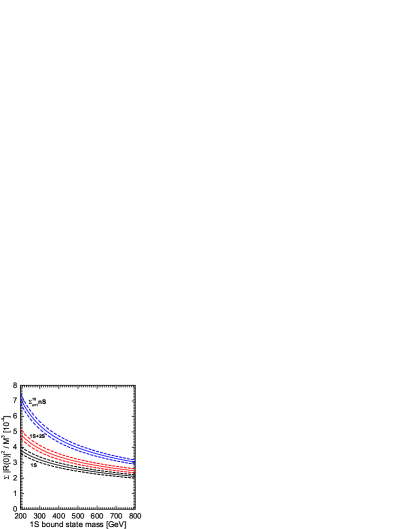
Figure 5: The bound state wavefunction at the origin factor $\sum|R(0)|^{2}/M^{3}$, as a function of the 1S bound state mass, as parameterized in Hagiwara:1990sq . The lower three lines are for the 1S wavefunction only, the middle group is the sum of the 1S and 2S wavefunctions, and the top group is the sum of the lowest 10 $S$-wave bound state wavefunctions. The solid lines are the $\Lambda^{(4)}_{\rm QCD}=300$ MeV parameterization and the dashed lines show the $\pm$40 MeV variations in this value.

In Figure 5 we plot the effective wavefunction at the origin factor given in Hagiwara:1990sq as a function of the 1S bound state mass. Three cases are shown in this plot: the contribution from the 1S bound state alone, the sum of the 1S and 2S bound states that we will use in numerical work, and the sum of the first 10 $S$-wave states. In each case, the 40 MeV variation in the QCD scale $\Lambda^{(4)}_{\rm QCD}$ (obtained by interpolation from the values given in ref. Hagiwara:1990sq ) is also plotted on the graph. Although the probability for producing higher-energy bound states drops sharply with higher $n$, their sum can add up to a significant enhancement to the overall production rate. It is not unlikely that we have underestimated the cross section for stoponium production and the rate of diphoton annihilation decays, but precise calculation of the additional enhancements will have to await a better understanding of stoponium spectroscopy.

In Figure 6

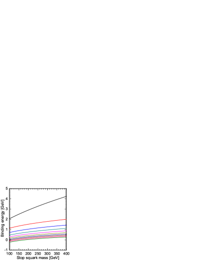
Figure 6: Binding energies $2m_{\tilde{t}}-M_{\eta_{\tilde{t}}}(nS)$ of the nS bound states of mass $M_{\eta_{\tilde{t}}}(nS)$ as a function of the constituent squark mass $m_{\tilde{t}}$. The top line is the 1S state, the second is the 2S state, and so on to the 10S state at the bottom. This plot uses the $\Lambda^{(4)}_{\rm QCD}=300$ MeV parameterization in ref. Hagiwara:1990sq .

we plot the binding energies of the first 10 $S$-wave bound states, computed using the parameterization in Hagiwara:1990sq . These are about 1% of the 1S bound state mass and significantly less for any other bound state. These differences are within the scale dependence of our result, and more importantly they will be below the energy resolution of the detectors. Therefore we will ignore the small binding energies in the calculation of the parton cross sections, taking $M=2m_{\tilde{t}}$ everywhere and ignoring any small differences in excited state masses.

IV.2 Numerical results for stoponium production

To integrate numerically the parton-level cross sections in equations (2.35), (2.43), and (2.46) using eq. (3.2), we will use the Martin-Stirling-Thorne-Watt (MSTW) 2008 NLO parton distribution functions Martin:2009iq , using their global best fits. These PDFs use the $\overline{\rm MS}$ subtraction scheme, and so we set $C_{gg}(z)=0$ in eq. (2.35) and $C_{gq}(z)=0$ in eq. (2.43). To be consistent with MSTW Martin:2009bu , we run $\alpha_{S}(Q)$ with two-loop beta function in the $n_{f}=5$ effective theory, starting from $\alpha_{S}(m_{Z})=0.12018$.

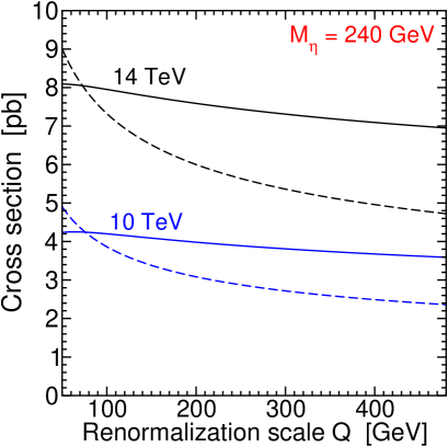
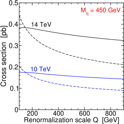
Figure 7: The scale dependence of the LO (dashed) and NLO (solid) $pp\rightarrow\eta_{\tilde{t}}+X$ cross sections for $M_{\eta_{\tilde{t}}}=240$ GeV (left) and 450 GeV (right), with the factorization scale $Q_{F}$ set equal to the renormalization scale $Q$, for $\sqrt{s}=14$ and 10 TeV.

In Fig. 7 we plot the renormalization scale dependence of the NLO $pp\rightarrow\eta_{\tilde{t}}+X$ cross section for two different masses $M_{\eta_{\tilde{t}}}=240$ and 450 GeV, varying $50\,{\rm GeV}<Q<480\,{\rm GeV}$ and $100\,{\rm GeV}<Q<900\,{\rm GeV}$ respectively as reasonable ranges for the choice of the common renormalization and factorization scale $Q=Q_{F}$. The figure shows the results for both $\sqrt{s}=10$ TeV and 14 TeV proton-proton colliders. These results show a significantly improved renormalization scale dependence for the NLO result compared to the LO cross section in each case.

We present the individual parton-induced contributions relative to the full hadronic cross section in Fig. 8, for $\sqrt{s}=14$ TeV proton-proton colliders and for the same masses and over the same ranges of $Q$ as in figure 7.

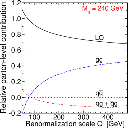
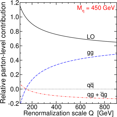
Figure 8: Relative contributions from each parton-level process relative to the total NLO $pp\rightarrow\eta_{\tilde{t}}+X$ for $M_{\eta_{\tilde{t}}}$ = 240 GeV (left) and 450 GeV (right), for $\sqrt{s}=14$ TeV, as a function of varying $Q=Q_{F}$, as in figure 7. The LO contribution is the order $\alpha_{S}^{2}$ result, the $gg$ contribution is due to real and virtual corrections to the leading order diagrams (the remaining part of eq. (2.35), the $qg+\bar{q}g$ contribution is from quark-gluon and antiquark-gluon scattering eq. (2.43), and the $q\bar{q}$ contribution is from quark-antiquark annihilation eq. (2.46).

Not surprisingly, for $Q=Q_{F}=M_{\eta_{\tilde{t}}}$, the relative contributions from each parton-level process are quite similar to those found for the toponium cross section in ref. Kuhn:1992qw . It is also interesting to note that for the scale choice $Q=Q_{F}\approx M_{\eta_{\tilde{t}}}/3$, the NLO $gg$, $qg+\bar{q}g$ and $q\bar{q}$ corrections are all simultaneously small. We have checked that this also holds for lower beam energies.

In Fig. 9,

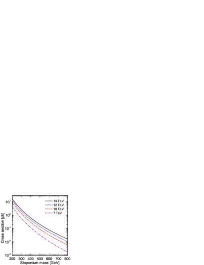
Figure 9: Results for NLO order cross sections for $pp\rightarrow\eta_{\tilde{t}}+X$ with $M_{\eta_{\tilde{t}}}$ between 200 and 800 GeV. Here we have set the factorization and renormalization scales equal to the stoponium mass, $Q=Q_{F}=M_{\eta_{\tilde{t}}}$.

we show the NLO $pp\rightarrow\eta_{\tilde{t}}+X$ cross section as a function of $M_{\eta_{\tilde{t}}}$, with the renormalization and factorization scales set equal to the stoponium mass. At this writing, the ultimate performance of the LHC is the subject of considerable speculation, so we show results for four different beam energies.

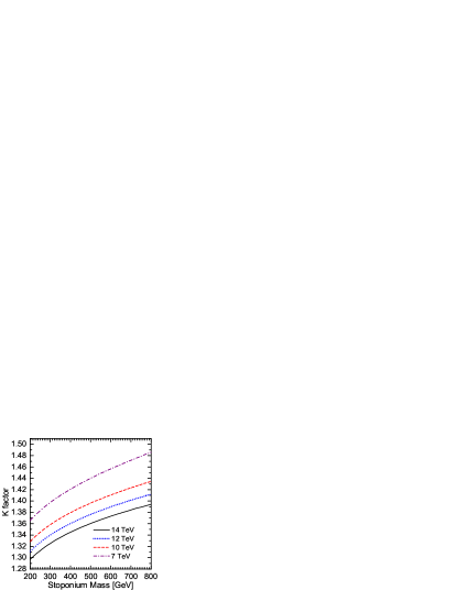
Figure 10: The K-factor, defined as the ratio of the NLO to LO cross sections for $pp\rightarrow\eta_{\tilde{t}}+X$, as a function of the stoponium mass $M_{\eta_{\tilde{t}}}$, computed with $Q=Q_{F}=M_{\eta_{\tilde{t}}}$. Results are shown for $\sqrt{s}=14$, 12, 10, and 7 TeV.

Figure 10 shows the corresponding K-factor, defined as the ratio of the next-to-leading order to the leading-order cross section, again with $Q=Q_{F}=M_{\eta_{\tilde{t}}}$. Our results show that the enhancement in the stoponium production cross section due to the NLO corrections with this scale choice is between 30% and 50%, depending on the energy of LHC, with larger enhancements for larger $M_{\eta_{\tilde{t}}}$ and for smaller $\sqrt{s}$.

IV.3 Numerical results for the diphoton final state

The observable signal for stoponium production is the diphoton peak produced by the decay $\eta_{\tilde{t}}\rightarrow\gamma\gamma$. The cross section for this signal is the product of the production cross section we have calculated above and the model-dependent branching ratio for diphoton decays of stoponium:

$$\sigma(pp\rightarrow\eta_{\tilde{t}}\rightarrow\gamma\gamma)=\sigma(pp\rightarrow\eta_{\tilde{t}}){\rm BR}(\eta_{\tilde{t}}\rightarrow\gamma\gamma)$$ (4.3)

Unfortunately, the $\gamma\gamma$ branching ratio is in general highly dependent on the parameter space of soft supersymmetry breaking. However, one can proceed by first considering the idealized model-independent case in which the total width is dominated by the gluon-gluon partial width. Then we can approximate the full width by the NLO width to hadrons ($gg+X$ or $q\bar{q}+X$), and calculate an approximate branching ratio:

$${\rm BR}(\eta_{\tilde{t}}\rightarrow\gamma\gamma)\approx\frac{\Gamma^{(1)}(\eta_{\tilde{t}}\rightarrow\gamma\gamma)}{\Gamma^{(1)}(\eta_{\tilde{t}}\rightarrow\mbox{hadrons})}\equiv R^{(1)},$$ (4.4)

where $\Gamma^{(1)}(\eta_{\tilde{t}}\rightarrow\mbox{hadrons})$ and $\Gamma^{(1)}(\eta_{\tilde{t}}\rightarrow\gamma\gamma)$ are the NLO partial widths. In our earlier paper Martin:2009dj , we found

$$R^{(1)} = \frac{8\alpha^{2}}{9\alpha_{S}^{2}}\bigg{\{}1+\frac{\alpha_{S}}{\pi}\bigg{[}-\frac{b_{0}}{2}\ln\biggl{(}\frac{Q^{2}}{M^{2}}\biggr{)}+\left(\frac{13\pi^{2}}{24}-\frac{199}{18}\right)N_{c}+\left(\frac{\pi^{2}}{4}-2-2\ln(2)\right)C_{F}$$ (4.5)

$$+\left(\frac{8}{9}(n_{f}+n_{t})+n_{t}h(4m_{t}^{2}/M^{2})+\frac{1}{6}\ln(2)\right)\bigg{]}\bigg{\}},$$

in which $M$ is the bound state mass, $n_{f}=5$, $n_{t}$ is zero or one depending on whether or not the mass of stoponium is large enough for top-antitop decays to be kinematically allowed, and the function $h(r)$ is defined by

$$h(r)=\frac{2}{9}(4-r)\sqrt{1-r}-\frac{8}{9}-\frac{2}{3}\ln(1+\sqrt{1-r})+\frac{2}{3}\ln(2).$$ (4.6)

The resulting idealized diphoton branching ratio $R^{(1)}$ is shown in Fig. 11.

Figure 11: The NLO branching ratio of stoponium to two photons in the idealized approximation that the hadronic partial width dominates the full width, from eq. (4.5). We have used $\alpha_{S}(m_{Z})=0.12018$ and set the renormalization scale equal to the stoponium mass.

(Here we have differed slightly from figure 8 of ref. Martin:2009dj by using values of $\alpha_{S}(Q)$ that follow from $\alpha_{S}(m_{Z})=0.12018$ to agree with those used in MSTW Martin:2009bu , using a slightly different two-loop running that includes the stop squark and includes the top quark only if the stop mass is greater than the top mass. We have also fixed the renormalization scale equal to the stoponium mass; the NLO scale variation is quite small as shown in Martin:2009dj .)

Now combining the NLO production cross section of fig. 9 with the NLO branching ratio of fig. 11, we find the idealized NLO $pp\rightarrow\eta_{\tilde{t}}+X\rightarrow\gamma\gamma+X$ cross section shown in fig. 12.

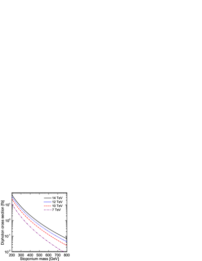
Figure 12: The NLO cross section times branching ratio for $pp\rightarrow\eta_{\tilde{t}}+X$ followed by $\eta_{\tilde{t}}\rightarrow\gamma\gamma$, in the idealized case that the stoponium decay width is dominated by the decays to gluons. The factorization and renormalization scales are set equal to the stoponium mass.

In this paper, we will not attempt a new study of the diphoton signal viability including backgrounds and after cuts. However, it is interesting to compare the corrected results we have found in the present paper and in Martin:2009dj to the corresponding LO results that were used as the basis for the study in ref. Martin:2008sv . There are several new effects taken into account in this paper. First, the NLO corrections to the diphoton branching ratio lead to a decrease of 30% to 35% when evaluated at $Q=M_{\eta_{\tilde{t}}}$. Second, and counteracting this, the NLO corrections to the production cross section lead to an increase as shown in fig. 10. Third, we are including here the effects of the $2S$ state as discussed in section IV.1. Also, ref. Martin:2008sv used a different set of parton distribution functions and a different $\alpha_{S}$. The net result of these effects is shown in Table 1, which compares the cross section (before cuts) used in the study ref. Martin:2008sv to that found here.

$M_{\eta_{\tilde{t}}}$ [GeV]	$\sigma\times\rm{BR}$ (fb, NLO)	$\sigma\times\rm{BR}$ (fb, LO in ref. Martin:2008sv )	ratio
235	22.4	23.1	0.969
240	20.5	21.0	0.974
255	15.8	16.0	0.989
270	12.3	12.3	1.00
400	2.14	1.94	1.10
450	1.24	1.09	1.13
500	0.750	0.647	1.16
600	0.307	0.255	1.20
700	0.141	0.113	1.24
800	0.0700	0.0549	1.27

Table 1: Comparison of cross section times branching ratio for $pp\rightarrow\eta_{\tilde{t}}+X\rightarrow\gamma\gamma+X$ in proton-proton collisions at $\sqrt{s}=14$ TeV, before cuts and in the idealized case that the hadronic partial width dominates the decay width of stoponium. The second column shows the results in fig. 12, and the third column shows the LO results as used in the study of the signal including cuts and LO backgrounds in ref. Martin:2008sv .

The results found here for the cross section times branching ratio are about equal to those used in Martin:2008sv for 235 GeV $<M_{\eta_{\tilde{t}}}<$ 270 GeV relevant for electroweak-scale baryogenesis models, and are somewhat larger for larger $M_{\eta_{\tilde{t}}}>400$ relevant for compressed supersymmetry models.

In the two motivated scenarios mentioned in the Introduction, there are somewhat different expectations for the reduction of the $pp\rightarrow\eta_{\tilde{t}}+X\rightarrow\gamma\gamma+X$ cross section compared to the idealized case just mentioned. For compressed supersymmetry compressed , in which enhancements to dark matter annihilation are mediated by $t$-channel stop squark exchange, the ground state stoponium will have a mass between about 400 GeV and 800 GeV, tending towards the former in models with less fine-tuning. The stoponium total width is indeed dominated by the hadronic partial width, which has a branching ratio that is typically more than 80% and usually of order 90% or even higher Martin:2008sv . The resulting diphoton cross sections can therefore be estimated from figure 12 simply by applying this correction factor as appropriate.

It is somewhat harder to make a prediction for the diphoton signal in models of electroweak-scale baryogenesis EWbaryogenesis ; EWbaryogenesisnew , because in those models the $h^{0}h^{0}$ decay width typically dominates if it is kinematically allowed, and also because the $WW$ and $ZZ$ modes are more significant. We have calculated the radiative corrections to $h^{0}h^{0}$ decay channel in ref. Martin:2009dj , but the weak vector boson decays are also significant (contributing up to about 30% of the total width for some choices of parameters). But to make a rough general statement about the cross section for diphoton annihilations, we can assume that the corrections to the weak decay channels should probably not be much larger than those for the hadronic decays; then the 30% reduction in $R^{(1)}$ over the leading order ratio leads us to conclude that a corresponding reduction in ${\rm BR}(\eta_{\tilde{t}}\rightarrow\gamma\gamma)$ is reasonable. These assumptions and the results in refs. Martin:2008sv ; Martin:2009dj allow us to make a conservative estimate for the next-to-leading order branching ratio in the electroweak baryogenesis models:

$${\rm BR}(\eta_{\tilde{t}}\rightarrow\gamma\gamma)\,\mathrel{\hbox to0.0pt{\lower 4.0pt\hbox{$\sim$}\hss}\raise 1.0pt\hbox{$>$}}\,\Biggl{\{}\begin{array}[]{l}1.5\times 10^{-3}\qquad(M<2m_{h^{0}}),\\ 5.3\times 10^{-4}\qquad(M>2m_{h^{0}}),\end{array}\Biggr{.}$$ (4.9)

Note that in these models, one expects $M_{\eta_{\tilde{t}}}$ between about 235 and 270 GeV, which happens to be in just the range where the decays to $h^{0}$ might become kinematically allowed. The branching ratio is highly dependent on the Higgs scalar boson mass because of its large partial width immediately above the threshold for Higgs pair production. Our resulting estimates for the stoponium diphoton annihilation cross section in the Electroweak Baryogenesis scenario are given in Table 2.

$M_{\eta_{\tilde{t}}}$ [GeV]	$\sigma(pp\rightarrow\eta_{\tilde{t}})$ [pb]	$\sigma_{\gamma\gamma}$, $M<2m_{h^{0}}$ [fb]	$\sigma_{\gamma\gamma}$, $M>2m_{h^{0}}$ [fb]
235	8.25	12	4.4
255	5.63	8.4	3.0
270	4.30	6.5	2.8

Table 2: Estimates of the NLO cross section for the production and subsequent diphoton annihilation decay of stoponium in a $\sqrt{s}=14$ TeV $pp$ collider, as a function of the stoponium mass in the electroweak baryogenesis model scenario. We have used approximate $\gamma\gamma$ branching ratios from eqs. (4.9).

V Outlook

In this paper, we have derived the NLO QCD corrections to the cross section for stoponium productions in hadronic collisions relevant for the LHC. These could be important in understanding an eventual discovery of, or limits on, stoponium through its diphoton annihilation decays. We found that when calculated at a scale $Q=M_{\eta_{\tilde{t}}}$, the corrections to the cross section are large and positive, partly canceling the large negative corrections in the diphoton branching ratio found in ref. Martin:2009dj . We also found that the NLO corrections to the cross section are small when evaluated at $Q\approx M_{\eta_{\tilde{t}}}/3$. For stoponium of mass 240 GeV (450 GeV), we found that reducing the center of mass energy from 14 TeV to 12 TeV will reduce the cross section by about 25% (30%), while reducing from 14 to 10 TeV will reduce the cross section by about 52% (55%), with of course larger reductions for heavier masses. We have not attempted here a detailed study improving on the estimate of the reach of the LHC based on LO signal and background in Martin:2008sv . One prerequisite for such an improvement is a better understanding of the Standard Model and detector diphoton backgrounds. There has been considerable study of the Standard Model high energy diphoton production at the LHC Balazs:1999yf -Balazs:2006cc , but focused on lower invariant masses relevant to a light Higgs scalar boson search. Fortunately, in the future the LHC will provide its own background estimate in the form of a sideband analysis, and this should be at least as robust as any calculation can be, at least for the purposes of bump-hunting.

The largest uncertainty in estimates of the stoponium cross section is clearly our lack of detailed understanding of stoponium energy levels and bound state matrix elements. In this paper, we used the parameterization of Hagiwara:1990sq for the wavefunction at the origin, but it must be recognized that this was obtained in part by a significant extrapolation from charmonium and bottomonium data. Even at the energy scales relevant for stoponium, the QCD binding potential is far from the semi-classical Coulomb form, and more work is needed to understand the relevant matrix elements. We have tried to remain relatively conservative by not including the possible effects from $S$-wave resonance production at the $3S$ level and beyond. An eventual discovery of stoponium in the diphoton channel will not only provide an accurate determination of the top squark mass, but an opportunity to use data to learn more about a QCD bound-state system in an energy range where calculations are under relatively better control than the known charmonium and bottomonium states.

Acknowledgments: We are grateful to Tim Tait for helpful conversation. This work was supported in part by the National Science Foundation grant number PHY-0757325.

References

- (1) M. Drees and M.M. Nojiri, Phys. Rev. Lett. 72, 2324 (1994) [hep-ph/9310209].
- (2) M. Drees and M.M. Nojiri, Phys. Rev. D 49, 4595 (1994) [hep-ph/9312213].
- (3) S.P. Martin, Phys. Rev. D 77, 075002 (2008) [hep-ph/0801.0237].
- (4) S.P. Martin and J.E. Younkin, Phys. Rev. D 80, 035026 (2009) [hep-ph/0901.4318].
- (5) C.R. Nappi, Phys. Rev. D 25, 84 (1982).
- (6) P. Moxhay and R.W. Robinett, Phys. Rev. D 32, 300 (1985).
- (7) M.J. Herrero, A. Mendez and T.G. Rizzo, Phys. Lett. B 200, 205 (1988).
- (8) V.D. Barger and W.Y. Keung, Phys. Lett. B 211, 355 (1988).
- (9) H. Inazawa and T. Morii, Phys. Rev. Lett. 70, 2992 (1993).
- (10) D.S. Gorbunov and V.A. Ilyin, JHEP 0011, 011 (2000) [hep-ph/0004092].
- (11) N. Fabiano, Eur. Phys. J. C 19, 547 (2001) [hep-ph/0103006].
- (12) Y. Kats and M.D. Schwartz, “Annihilation decays of bound states at the LHC,” [hep-ph/0912.0526].
- (13) S.P. Martin, Phys. Rev. D 75, 115005 (2007) [hep-ph/0703097], Phys. Rev. D 76, 095005 (2007) [hep-ph/0707.2812]. Phys. Rev. D 78, 055019 (2008) [hep-ph/0807.2820].
- (14) J.R. Espinosa, M. Quiros and F. Zwirner, Phys. Lett. B 307, 106 (1993) [hep-ph/9303317], M.S. Carena, M. Quiros and C.E.M. Wagner, Phys. Lett. B 380, 81 (1996) [hep-ph/9603420], Nucl. Phys. B 524, 3 (1998) [hep-ph/9710401], J.R. Espinosa, Nucl. Phys. B 475, 273 (1996) [hep-ph/9604320], D. Bodeker, P. John, M. Laine and M. G. Schmidt, Nucl. Phys. B 497, 387 (1997) [hep-ph/9612364], M.S. Carena, M. Quiros, A. Riotto, I. Vilja and C.E.M. Wagner, Nucl. Phys. B 503, 387 (1997) [hep-ph/9702409], J.M. Cline, M. Joyce and K. Kainulainen, Phys. Lett. B 417, 79 (1998) [Erratum-ibid. B 448, 321 (1999)] [hep-ph/9708393], JHEP 0007, 018 (2000) [hep-ph/0006119], J.M. Cline and G.D. Moore, Phys. Rev. Lett. 81, 3315 (1998) [hep-ph/9806354], M.S. Carena, M. Quiros, M. Seco and C.E.M. Wagner, Nucl. Phys. B 650, 24 (2003) [hep-ph/0208043].
- (15) M. Carena, G. Nardini, M. Quiros and C.E.M. Wagner, JHEP 0810, 062 (2008) [hep-ph/0806.4297]. M. Carena, A. Freitas and C.E.M. Wagner, JHEP 0810, 109 (2008) [hep-ph/0808.2298]. M. Carena, G. Nardini, M. Quiros and C.E.M. Wagner, Nucl. Phys. B 812, 243 (2009), [hep-ph/0809.3760]. A. Menon and D.E. Morrissey, Phys. Rev. D 79, 115020 (2009) [hep-ph/0903.3038].
- (16) J.H. Kühn and E. Mirkes, Phys. Rev. D 48, 179 (1993) [hep-ph/9301204].
- (17) F. Abe et al. [CDF Collaboration], Phys. Rev. Lett. 79, 572 (1997),
- (18) V.M. Abazov et al. [D0 Collaboration], Phys. Rev. Lett. 94, 232001 (2005) [Erratum-ibid. 100, 049902 (2008)] [hep-ex/0502030].
- (19) D.E. Acosta et al. [CDF Collaboration], Phys. Rev. Lett. 88, 161802 (2002).
- (20) P. Artoisenet, J.M. Campbell, J.P. Lansberg, F. Maltoni and F. Tramontano, Phys. Rev. Lett. 101, 152001 (2008) [hep-ph/0806.3282].
- (21) A. Petrelli, M. Cacciari, M. Greco, F. Maltoni and M.L. Mangano, Nucl. Phys. B 514, 245 (1998) [hep-ph/9707223].
- (22) M. Kramer, Prog. Part. Nucl. Phys. 47, 141 (2001) [hep-ph/0106120].
- (23) N. Brambilla et al. [Quarkonium Working Group], “Heavy quarkonium physics,” [hep-ph/0412158].
- (24) J.P. Lansberg, Int. J. Mod. Phys. A 21, 3857 (2006) [hep-ph/0602091].
- (25) J.P. Lansberg, Eur. Phys. J. C 61, 693 (2009) [hep-ph/0811.4005].
- (26) G.P. Lepage, L. Magnea, C. Nakhleh, U. Magnea and K. Hornbostel, Phys. Rev. D 46, 4052 (1992) [hep-lat/9205007].
- (27) G.T. Bodwin, E. Braaten and G.P. Lepage, Phys. Rev. D 51, 1125 (1995) [Erratum-ibid. D 55, 5853 (1997)] [hep-ph/9407339].
- (28) A.A. Affolder et al. [CDF Collaboration], Phys. Rev. Lett. 85, 2886 (2000) [hep-ex/0004027]. A. Abulencia et al. [CDF Collaboration], Phys. Rev. Lett. 99, 132001 (2007) [hep-ex/0704.0638].
- (29) A. Adare et al. [PHENIX Collaboration], Phys. Rev. Lett. 98, 232002 (2007) [hep-ex/0611020].
- (30) F. Maltoni and A.D. Polosa, Phys. Rev. D 70, 054014 (2004) [hep-ph/0405082].
- (31) K. Hagiwara, K. Kato, A.D. Martin and C.K. Ng, Nucl. Phys. B 344, 1 (1990).
- (32) See e.g. R.D. Field, “Applications of Perturbative QCD,” Addison-Wesley (1989) (Frontiers in physics, 77) or R.K. Ellis, W.J. Stirling, and B.R. Webber, “QCD and Collider Physics”, Cambridge University Press (1996).
- (33) A.D. Martin, W.J. Stirling, R.S. Thorne and G. Watt, Eur. Phys. J. C 63, 189 (2009) [hep-ph/0901.0002].
- (34) A.D. Martin, W.J. Stirling, R.S. Thorne and G. Watt, [hep-ph/0905.3531].
- (35) C. Balazs, P. Nadolsky, C. Schmidt and C.P. Yuan, Phys. Lett. B 489, 157 (2000) [hep-ph/9905551].
- (36) T. Binoth, J.P. Guillet, E. Pilon and M. Werlen, Eur. Phys. J. C 16, 311 (2000) [hep-ph/9911340].
- (37) Z. Bern, A. De Freitas and L.J. Dixon, JHEP 0109, 037 (2001) [hep-ph/0109078], Z. Bern, L.J. Dixon and C. Schmidt, Phys. Rev. D 66, 074018 (2002) [hep-ph/0206194].
- (38) C. Balazs, E.L. Berger, P.M. Nadolsky and C.P. Yuan, Phys. Lett. B 637, 235 (2006) [hep-ph/0603037], Phys. Rev. D 76, 013009 (2007) [hep-ph/0704.0001].