UTHEP-600 RIKEN-TH-177

Light-cone Gauge Superstring Field Theory
and Dimensional Regularization II

Yutaka Baba^a, Nobuyuki Ishibashi^b, Koichi Murakami^a

^aTheoretical Physics Laboratory, Nishina Center, RIKEN,
Wako, Saitama 351-0198, Japan

^bInstitute of Physics, University of Tsukuba,
Tsukuba, Ibaraki 305-8571, Japan

We propose a dimensional regularization scheme to deal with the divergences caused by colliding supercurrents inserted at the interaction points, in the light-cone gauge NSR superstring field theory. We formulate the theory in $d$ dimensions and define the amplitudes as analytic functions of $d$. With an appropriately chosen three-string interaction term and large negative $d$, the tree level amplitudes for the (NS,NS) closed strings can be recast into a BRST invariant form, using the superconformal field theory proposed in Ref. [1]. We show that in the limit $d\rightarrow 10$ they coincide with the results of the first quantized theory. Therefore we obtain the desired results without adding any contact interaction terms to the action.

1 Introduction

Perturbative expansion of amplitudes in the light-cone gauge NSR superstring field theory [2, 3] involves divergences even at the tree level. Transverse supercurrents are inserted at the interaction points of the joining-splitting interaction and divergences arise when they get close to each other. Similar divergences exist in other superstring field theories  [4, 5, 6, 7, 8].

In the previous paper [9] we have proposed a dimensional regularization scheme to deal with these divergences. In the light-cone gauge, one can define the theory in $d~{}(d\neq 10)$ dimensions. Taking $d$ to be largely negative, we can make the tree level amplitudes finite. Defining the amplitudes for such $d$, one can obtain the amplitudes for $d=10$ by analytic continuation. Since what matters is the Virasoro central charge on the worldsheet, one can effectively change $d$ also by using conformal field theory other than that for the transverse variables $X^{i},\psi^{i},\tilde{\psi}^{i}$. In Ref. [9], we have proposed one such scheme and shown that the results of the first quantized formulation can be reproduced by such a procedure, in the case of the four string amplitudes.

In order for the dimensional regularization scheme to be effective, it should preserve as many symmetries of the theory as possible. In Refs. [10, 1], we have shown that the light-cone gauge string field theory in noncritical spacetime dimensions corresponds to a BRST invariant worldsheet theory with the longitudinal variables and the ghosts. Since the BRST symmetry on the worldsheet is supposed to be related to the gauge symmetry of the string field theory, these results imply that the dimensional regularization can be carried out with the gauge symmetry preserved.

In this paper, we would like to propose a dimensional regularization scheme for the light-cone gauge NSR superstring field theory, in which the results of Ref. [1] can be used. We just formulate the theory in $d$ dimensions and define the amplitudes as analytic functions of $d$. In this paper, we deal with closed string field theory and restrict ourselves to the amplitudes with only the (NS,NS) external lines. We show that the tree level amplitudes can be recast into a BRST invariant form using the superconformal field theory proposed in Ref. [1]. In this form, it is easy to show that the amplitudes coincide with the results of the first quantized formulation without any need for the modification of the action by adding the counterterms.

The organization of this paper is as follows. In section 2, we study the light-cone gauge closed string field theory for NSR superstrings defined in spacetime dimension $d\neq 10$. We show that the tree level amplitudes become well-defined by setting $d$ to be a sufficiently large negative value. In section 3, we rewrite the tree level amplitudes into a BRST invariant form, using the superconformal field theory for the longitudinal variables $X^{\pm},\psi^{\pm},\tilde{\psi}^{\pm}$ formulated in Ref. [1] and introducing the ghost fields. In section 4, we show that the tree level amplitudes coincide with the results of the first quantized formulation in the limit $d\to 10$. Section 5 is devoted to conclusions and discussions. In appendix A, we explain the details of the action of the superstring field theory given in section 2. In appendix B, we present the calculations to obtain the tree level amplitudes. In appendix C, we present a proof of the property satisfied by the correlation functions of $\psi^{-}$, which is used in section 3.

2 Amplitudes for $d\neq 10$ and Dimensional Regularization

In order to dimensionally regularize the light-cone gauge NSR string field theory, we take the worldsheet theory to be the free theory of the transverse variables $X^{i},\psi^{i},\tilde{\psi}^{i}$ $(i=1,\cdots,d-2)$. The light-cone gauge string field theory can be defined even for $d\neq 10$. In this paper, we concentrate on the closed strings in the (NS,NS) sector and the action is given in the form

$$S = \int dt\left[\frac{1}{2}\int d1d2\left\langle R\left(1,2\right)|\Phi(t)\right\rangle_{1}\left(i\frac{\partial}{\partial t}-\frac{L_{0}^{\mathrm{LC}(2)}+\tilde{L}_{0}^{\mathrm{LC}(2)}-\frac{d-2}{8}}{\alpha_{2}}\right)\left|\Phi(t)\right\rangle_{2}\right.$$ (2.1)

$$\hphantom{\int dt\frac{1}{2}\int d1d2}\left.\vphantom{\left(i\frac{\partial}{\partial t}-\frac{L_{0}^{\mathrm{LC}\left(2\right)}+\tilde{L}_{0}^{\mathrm{LC}\left(2\right)}-\frac{d-2}{8}}{\alpha_{2}}\right)}{}+\frac{2g}{3}\int d1d2d3\left\langle V_{3}\left(1,2,3\right)|\Phi(t)\right\rangle_{1}\left|\Phi(t)\right\rangle_{2}\left|\Phi(t)\right\rangle_{3}\right].$$

In order for the amplitudes of the light-cone gauge string field theory to be rewritten into a BRST invariant form, the three-string interaction term should be taken appropriately. Details of the action (2.1) are explained in appendix A.

Starting from this action, the tree level $N$-string amplitudes can be calculated perturbatively. A typical tree level $N$-string diagram is depicted in Fig. 1 $(a)$ for the $N=5$ case. On such string diagrams, we introduce a complex $\rho$-coordinate as usual. The $N$-string tree diagram is mapped to the complex $z$-plane in Fig. 1 $(b)$ via the Mandelstam mapping $\rho(z)$ defined as

$$\rho(z)=\sum_{r=1}^{N}\alpha_{r}\ln(z-Z_{r})~{},$$ (2.2)

where the external lines are mapped to the regions $z\sim Z_{r}$ $(r=1,\ldots,N)$. We denote the interaction points by $z_{I}$ $(1,\ldots,N-2)$ which determined by $\partial\rho(z_{I})=0$.

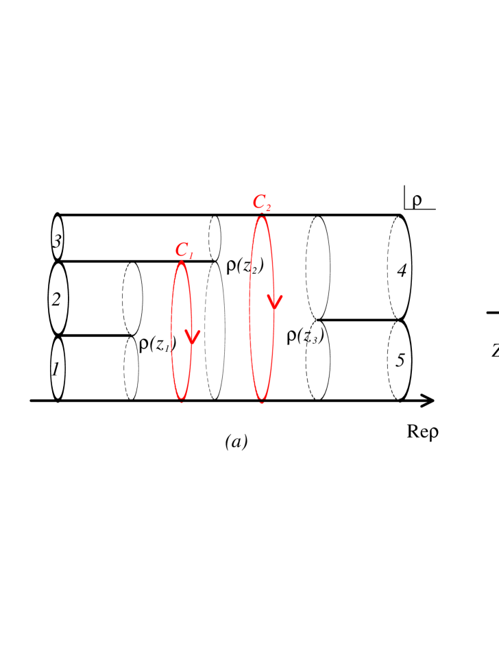
Figure 1: In $(a)$ is depicted a typical $N$-string tree diagram with $N=5$, on which a complex coordinate $\rho$ is introduced. Via the Mandelstam mapping $\rho(z)$, the $\rho$-plane is mapped to the complex $z$-plane in $(b)$. $\rho(z_{I})$ $(I=1,2,3)$ are the interaction points on the $\rho$-plane. For the string diagram $(a)$, the complex Schwinger parameters $\mathcal{T}_{\mathcal{I}}$ $(\mathcal{I}=1,2)$ are given by $\mathcal{T}_{1}=\rho(z_{2})-\rho(z_{1})$ and $\mathcal{T}_{2}=\rho(z_{3})-\rho(z_{2})$. $C_{\mathcal{I}}$ are the contours of the integrals in eq.(3.30) for this string diagram.

The resulting amplitudes can be expressed as an integral over the moduli space of the string diagram as

$$\mathcal{A}_{N}=\left(4ig\right)^{N-2}\int\left(\prod_{\mathcal{I}=1}^{N-3}\frac{d^{2}\mathcal{T}_{\mathcal{I}}}{4\pi}\right)F_{N}\left(\mathcal{T}_{\mathcal{I}},\bar{\mathcal{T}_{\mathcal{I}}}\right)~{},$$ (2.3)

where $\mathcal{T}_{\mathcal{I}}$ $(\mathcal{I}=1,\ldots,N-3)$ denotes the complex Schwinger parameter for the $\mathcal{I}$-th internal propagator. $\mathcal{T}_{\mathcal{I}}$’s constitute the $N-3$ complex moduli parameters of the tree string diagram with $N$ external strings, and are the $N$-string generalization of $\mathcal{T}$ given in eq.(B.13) for the four-string case. The integral in eq.(2.3) is taken over the whole moduli space of the string diagram. The integrand $F_{N}(\mathcal{T}_{\mathcal{I}},\bar{\mathcal{T}}_{\mathcal{I}})$ is described by using the worldsheet field theory for the transverse variables [9] as

$$F_{N}\left(\mathcal{T}_{\mathcal{I}},\bar{\mathcal{T}_{\mathcal{I}}}\right) = \left(2\pi\right)^{2}\delta\Biggl{(}\sum_{r=1}^{N}p_{r}^{+}\Biggr{)}\delta\Biggl{(}\sum_{r=1}^{N}p_{r}^{-}\Biggr{)}\mathrm{sgn}\Biggl{(}\prod_{r=1}^{N}\alpha_{r}\Biggr{)}e^{-\frac{d-2}{16}\Gamma\left[\ln\left(\partial\rho\bar{\partial}\bar{\rho}\right)\right]}$$ (2.4)

$$\quad\times\left\langle\prod_{I=1}^{N-2}\left[\left(\partial^{2}\rho\left(z_{I}\right)\bar{\partial}^{2}\bar{\rho}\left(\bar{z}_{I}\right)\right)^{-\frac{3}{4}}T_{F}^{\mathrm{LC}}\left(z_{I}\right)\tilde{T}_{F}^{\mathrm{LC}}\left(\bar{z}_{I}\right)\right]\prod_{r=1}^{N}V_{r}^{\mathrm{LC}}\right\rangle.$$

Here $\langle\mathcal{O}\rangle$ denotes the expectation value of the operator $\mathcal{O}$ on the complex $z$-plane, defined as

$$\left\langle\mathcal{O}\right\rangle=\frac{\displaystyle\int\left[dX^{i}d\psi^{i}d\tilde{\psi}^{i}\right]e^{-S_{\mathrm{LC}}}\,\mathcal{O}}{\displaystyle\int\left[dX^{i}d\psi^{i}d\tilde{\psi}^{i}\right]e^{-S_{\mathrm{LC}}}}~{},$$ (2.5)

and $S_{\mathrm{LC}}$ denotes the worldsheet action of the light-cone gauge NSR superstring. $V_{r}^{\mathrm{LC}}$ is the vertex operator defined in eq.(B.24), and $T^{\mathrm{LC}}_{F}(z)$ is the transverse supercurrent. $\Gamma\left[\ln\left(\partial\rho\bar{\partial}\bar{\rho}\right)\right]$ is given in Ref. [10] as

$$e^{-\Gamma\left[\ln\left(\partial\rho\bar{\partial}\bar{\rho}\right)\right]}=\left|\sum_{r=1}^{N}\alpha_{r}Z_{r}\right|^{4}\prod_{r=1}^{N}\left(|\alpha_{r}|^{-2}e^{-2\mathop{\mathrm{Re}}\bar{N}^{rr}_{00}}\right)\prod_{I=1}^{N-2}\left|\partial^{2}\rho(z_{I})\right|^{-1}~{},$$ (2.6)

where $\bar{N}^{rr}_{00}$ denotes a Neumann coefficient defined as

$$\bar{N}^{rr}_{00}=\frac{\tau^{(r)}_{0}+i\beta_{r}}{\alpha_{r}}-\sum_{s\neq r}\frac{\alpha_{s}}{\alpha_{r}}\ln\left(Z_{r}-Z_{s}\right)~{},\qquad\tau_{0}^{(r)}+i\beta_{r}\equiv\rho(z_{I^{(r)}})~{}.$$ (2.7)

Here $z_{I^{(r)}}$ denotes the interaction point on the $z$-plane at which the $r$-th string interacts. Which of $z_{I}$ should be identified with $z_{I^{(r)}}$ depends on the channel. For example, $z_{I^{(1)}}=z_{I^{(2)}}=z_{1}$, $z_{I^{(3)}}=z_{2}$ and $z_{I^{(4)}}=z_{I^{(5)}}=z_{3}$ for the string diagram depicted in Fig. 1 $(a)$, while $z_{I^{(1)}}=z_{1}$, $z_{I^{(2)}}=z_{I^{(3)}}=z_{2}$ and $z_{I^{(3)}}=z_{I^{(4)}}=z_{3}$ for the string diagram in Fig. 2. See appendix B for details of the calculations to obtain the expression (2.3) of the amplitude.

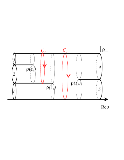
Figure 2: A $5$-string tree diagram in a different channel from that in Fig. 1 $(a)$.

In general, $F_{N}\left(\mathcal{T}_{\mathcal{I}},\bar{\mathcal{T}_{\mathcal{I}}}\right)$ in eq.(2.4) is singular in the limit $z_{I}\rightarrow z_{J}$. Nevertheless, if $d$ is taken to be a sufficiently large negative value as a regularization, $F_{N}\left(\mathcal{T}_{\mathcal{I}},\bar{\mathcal{T}_{\mathcal{I}}}\right)$ vanishes in the limit $z_{I}\rightarrow z_{J}$. It is because in this limit, $e^{-\frac{d-2}{16}\Gamma\left[\ln\left(\partial\rho\bar{\partial}\bar{\rho}\right)\right]}$ behaves as $\left|z_{I}-z_{J}\right|^{-\frac{d-2}{8}}$ and the contributions of the other operators are with $d$ independent power of $\left|z_{I}-z_{J}\right|$. The other singularities can be dealt with by the analytic continuation of the external momenta $p_{r}$. Thus we can define the integral in eq.(2.3) for such $d$ and obtain the dimensionally regularized amplitudes.

3 BRST Invariant Form of Amplitudes

In this section, we would like to show that the amplitude (2.3) can be recast into a BRST invariant form using the superconformal field theory proposed in Ref. [1]. We basically follow the procedure given in Refs. [11, 12, 9, 10]. In the subsequent calculations, we will not care about the overall numerical factor.

We first note that from eq.(2.6) one can obtain the relation

$$e^{-\frac{d-2}{16}\Gamma\left[\ln\left(\partial\rho\bar{\partial}\bar{\rho}\right)\right]} = e^{-\frac{d-10}{16}\Gamma\left[\ln\left(\partial\rho\bar{\partial}\bar{\rho}\right)\right]}\left|\sum_{s=1}^{N}\alpha_{s}Z_{s}\right|^{2}$$ (3.1)

$$\quad\times\prod_{r=1}^{N}\left(\left|\alpha_{r}\right|^{-1}e^{-\mathop{\mathrm{Re}}\bar{N}_{00}^{rr}}\right)\prod_{I=1}^{N-2}\left(\partial^{2}\rho\left(z_{I}\right)\bar{\partial}^{2}\bar{\rho}\left(\bar{z}_{I}\right)\right)^{-\frac{1}{4}}.$$

By using this relation, eq.(2.4) becomes

$$F_{N}\left(\mathcal{T}_{\mathcal{I}},\bar{\mathcal{T}_{\mathcal{I}}}\right)\sim\left(2\pi\right)^{2}\delta\Biggl{(}\sum_{r=1}^{N}p_{r}^{+}\Biggr{)}\delta\Biggl{(}\sum_{r=1}^{N}p_{r}^{-}\Biggr{)}e^{-\frac{d-10}{16}\Gamma\left[\ln\left(\partial\rho\bar{\partial}\bar{\rho}\right)\right]}\left|\sum_{s=1}^{N}\alpha_{s}Z_{s}\right|^{2}$$ (3.2)

$$\qquad\times\left\langle\prod_{I=1}^{N-2}\left[\left(\partial^{2}\rho\left(z_{I}\right)\bar{\partial}^{2}\bar{\rho}\left(\bar{z}_{I}\right)\right)^{-1}T_{F}^{\mathrm{LC}}\left(z_{I}\right)\tilde{T}_{F}^{\mathrm{LC}}\left(\bar{z}_{I}\right)\right]\prod_{r=1}^{N}\left(\alpha_{r}^{-1}V_{r}^{\mathrm{LC}}e^{-\mathop{\mathrm{Re}}\bar{N}^{rr}_{00}}\right)\right\rangle.$$

3.1 Ghosts

In order to obtain a BRST invariant form, we need to introduce the longitudinal variables and the ghosts. Let us first consider the ghost fields $b,c,\beta,\gamma$ and their anti-holomorphic counterparts. The ghosts can be introduced [9] by multiplying $F_{N}$ by

$$\int\left[d(\mbox{ghost})\right]e^{-S_{\mathrm{gh}}}\lim_{z\to\infty}\left(\frac{1}{|z|^{4}}c(z)\tilde{c}(\bar{z})\right)$$

$$\quad\times\prod_{I=1}^{N-2}\left[b\left(z_{I}\right)\tilde{b}\left(\bar{z}_{I}\right)e^{\phi}\left(z_{I}\right)e^{\tilde{\phi}}\left(\bar{z}_{I}\right)\right]\prod_{r=1}^{N}\left[c\left(Z_{r}\right)\tilde{c}\left(\bar{Z}_{r}\right)e^{-\phi}\left(Z_{r}\right)e^{-\tilde{\phi}}\left(\bar{Z}_{r}\right)\right],$$ (3.3)

which is just a constant. Here $S_{\mathrm{gh}}$ denotes the worldsheet action for the ghost fields. We have used a shorthand notation $d(\mbox{ghost})=dbdcd\beta d\gamma d\tilde{b}d\tilde{c}d\tilde{\beta}d\tilde{\gamma}$, and bosonized $\beta\gamma$-ghosts [13] as

$$\beta=e^{-\phi}\partial\xi~{},\qquad\gamma=\eta e^{\phi}~{}.$$ (3.4)

3.2 Longitudinal variables

Next, let us consider the longitudinal variables $X^{\pm},\psi^{\pm},\tilde{\psi}^{\pm}$, which are the component fields of the superfields $\mathcal{X}^{\pm}$ given as

$$\mathcal{X}^{\pm}(\mathbf{z},\bar{\mathbf{z}})=X^{\pm}+i\theta\psi^{\pm}+i\bar{\theta}\tilde{\psi}^{\pm}+i\theta\bar{\theta}F^{\pm}~{}.$$ (3.5)

We can rewrite the correlation function on the right hand side of eq.(3.2) using the $X^{\pm}$ CFT [1]. The $X^{\pm}$ CFT is a superconformal field theory of the longitudinal variables, with the action

$$S_{\pm}\equiv-\frac{1}{2\pi}\int d^{2}\mathbf{z}\left(\bar{D}\mathcal{X}^{+}D\mathcal{X}^{-}+\bar{D}\mathcal{X}^{-}D\mathcal{X}^{+}\right)+\frac{d-10}{8}\Gamma_{\mathrm{super}}\left[\Phi\right]~{}.$$ (3.6)

Here $\Gamma_{\mathrm{super}}\left[\Phi\right]$ is the super Liouville action,

$$\frac{d-10}{8}\Gamma_{\mathrm{super}}\left[\Phi\right]=-\frac{d-10}{16\pi}\int d^{2}\mathbf{z}\bar{D}\Phi D\Phi\;,$$ (3.7)

and $\Phi$ is the superfield given by

$$\Phi\left(\mathbf{z},\bar{\mathbf{z}}\right) = \ln\left(-4\left(D\Theta^{+}\right)^{2}\left(\mathbf{z}\right)\left(\bar{D}\bar{\Theta}^{+}\right)^{2}\left(\bar{\mathbf{z}}\right)\right)\;,$$

$$\Theta^{+}\left(\mathbf{z}\right) = \frac{D\mathcal{X}^{+}}{(\partial\mathcal{X}^{+})^{\frac{1}{2}}}\left(\mathbf{z}\right)\;.$$ (3.8)

In this superconformal field theory, we have

$$\int\left[dX^{\pm}d\psi^{\pm}d\tilde{\psi}^{\pm}\right]e^{-S_{\pm}}\,F\left[X^{+},\psi^{+},\tilde{\psi}^{+}\right]\prod_{r=1}^{N}e^{-ip_{r}^{+}X^{-}}\left(Z_{r},\bar{Z}_{r}\right)$$

$$\qquad\sim e^{-\frac{d-10}{16}\Gamma\left[\ln\left(\partial\rho\bar{\partial}\bar{\rho}\right)\right]}F\left[-\frac{i}{2}\left(\rho+\bar{\rho}\right),0,0\right]~{},$$ (3.9)

for any functional $F\left[X^{+},\psi^{+},\tilde{\psi}^{+}\right]$ of $X^{+}$, $\psi^{+}$, $\tilde{\psi}^{+}$. This can be obtained from eq.(2.11) of Ref. [1] by setting all the Grassmann odd coordinates of the external lines $\Theta_{r}$ $(r=1,\ldots,N)$ to be $0$. By using eq.(3.9), we obtain

$$\int[dX^{\pm}d\psi^{\pm}d\tilde{\psi}^{\pm}]e^{-S_{\pm}}\,\prod_{r=1}^{N}\left[V_{r}^{\prime\mathrm{DDF}}\left(Z_{r},\bar{Z}_{r}\right)e^{\frac{d-10}{16}\frac{i}{p^{+}_{r}}X^{+}}(z_{I^{(r)}},\bar{z}_{I^{(r)}})\right]$$

$$\qquad\sim(2\pi)^{2}\delta\Biggl{(}\sum_{r=1}^{N}p_{r}^{+}\Biggr{)}\delta\Biggl{(}\sum_{r=1}^{N}p_{r}^{-}\Biggr{)}e^{-\frac{d-10}{16}\Gamma\left[\ln\left(\partial\rho\bar{\partial}\bar{\rho}\right)\right]}\prod_{r=1}^{N}\left(\alpha_{r}^{-1}V_{r}^{\mathrm{LC}}e^{-\mathop{\mathrm{Re}}\bar{N}^{rr}_{00}}\right)~{}.$$ (3.10)

The vertex operator $V^{\prime\mathrm{DDF}}_{r}$ on the left hand side is defined as

$$V_{r}^{\prime\mathrm{DDF}}\left(Z_{r},\bar{Z}_{r}\right)\equiv:V_{r}^{\mathrm{DDF}}e^{-\frac{d-10}{16}\frac{i}{p_{r}^{+}}X^{+}}\left(Z_{r},\bar{Z}_{r}\right):~{},$$ (3.11)

and $V_{r}^{\mathrm{DDF}}$ is the vertex operator for the DDF state which corresponds to $V_{r}^{\mathrm{LC}}$ in eq.(B.24), defined as

$$V_{r}^{\mathrm{DDF}}\left(Z_{r},\bar{Z}_{r}\right)$$ (3.12)

$$\equiv A_{-n_{1}}^{i_{1}(r)}\cdots\tilde{A}_{-\tilde{n}_{1}}^{\tilde{\imath}_{1}(r)}\cdots B_{-s_{1}}^{j_{1}(r)}\cdots\tilde{B}_{-\tilde{s}_{1}}^{\tilde{\jmath}_{1}(r)}\cdots\,e^{ip_{r}^{i}X^{i}-ip_{r}^{+}X^{-}-i\left(p_{r}^{-}-\frac{N_{r}}{p_{r}^{+}}\right)X^{+}}\left(Z_{r},\bar{Z}_{r}\right).~{}~{}~{}$$

Here $A^{i(r)}_{-n}$ and $B^{i(r)}_{-s}$ denote the DDF operators given by

$$A_{-n}^{i(r)} \equiv \oint_{Z_{r}}\frac{dz}{2\pi i}\left(i\partial X^{i}+\frac{n}{p_{r}^{+}}\psi^{i}\psi^{+}\right)e^{-i\frac{n}{p_{r}^{+}}X_{L}^{+}}(z)\ ,$$

$$B_{-s}^{i(r)} \equiv \oint_{Z_{r}}\frac{dz}{2\pi i}\left(\psi^{i}-\partial X^{i}\frac{\psi^{+}}{\partial X^{+}}-\frac{1}{2}\psi^{i}\frac{\psi^{+}\partial\psi^{+}}{\left(\partial X^{+}\right)^{2}}\right)\left(\frac{i\partial X^{+}}{p_{r}^{+}}\right)^{\frac{1}{2}}e^{-i\frac{s}{p_{r}^{+}}X_{L}^{+}}(z)~{},$$ (3.13)

and $N_{r}$ is the level number,

$$N_{r}\equiv\sum_{i}n_{i}+\sum_{j}s_{j}=\sum_{k}\tilde{n}_{k}+\sum_{l}\tilde{s}_{l}~{}.$$ (3.14)

The on-shell condition (B.17) implies that $p_{r}^{-}$ is given as

$$p_{r}^{-}=\frac{1}{p_{r}^{+}}\left(\frac{1}{2}\vec{p}_{r}^{\;2}+N_{r}-\frac{d-2}{16}\right).$$ (3.15)

We need some care to precisely define the operator $e^{\frac{d-10}{16}\frac{i}{p_{r}^{+}}X^{+}}(z_{I^{(r)}},\bar{z}_{I^{(r)}})$ in the path integral (3.10) with the action $S_{\pm}$. The argument $z_{I^{(r)}}$ itself depends on $\alpha_{s},Z_{s}$ and it is influenced by the presence of other operators. Here we take the expression

$$\oint_{z_{I^{(r)}}}\frac{d\mathbf{z}}{2\pi i}D\Phi(\mathbf{z})\oint_{\bar{z}_{I^{(r)}}}\frac{d\bar{\mathbf{z}}}{2\pi i}\bar{D}\Phi(\bar{\mathbf{z}})e^{\frac{d-10}{16}\frac{i}{p^{+}_{r}}\mathcal{X}^{+}}(\mathbf{z},\bar{\mathbf{z}})~{}.$$ (3.16)

As the definition of this operator, this coincides with $e^{\frac{d-10}{16}\frac{i}{p_{r}^{+}}X^{+}}(z_{I^{(r)}},\bar{z}_{I^{(r)}})$ under the identification $X^{+}\sim-\frac{i}{2}\left(\rho+\bar{\rho}\right)$; $\psi^{+},\tilde{\psi}^{+}\sim 0$, which can be done in the path integral of the form on the left hand side of eq.(3.9).

We can introduce the longitudinal variables by substituting eqs.(3.10) and (3.16) into eq.(3.2). With the ghost variables introduced above, and using the relation $\frac{b}{\partial^{2}\rho}(z_{I})=\oint_{z_{I}}\frac{dz}{2\pi i}\frac{b}{\partial\rho}(z)$, we obtain

$$F_{N} \sim \int\left[dXd\psi d\tilde{\psi}d(\mbox{ghost})\right]e^{-S}\lim_{z\to\infty}\left(\frac{1}{|z|^{4}}c(z)\tilde{c}(\bar{z})\right)\left|\sum_{r=1}^{N}\alpha_{r}Z_{r}\right|^{2}$$ (3.17)

$$\quad\times\prod_{r=1}^{N}\left[ce^{-\phi}\tilde{c}e^{-\tilde{\phi}}V_{r}^{\prime\mathrm{DDF}}\left(Z_{r},\bar{Z}_{r}\right)\oint_{z_{I^{(r)}}}\frac{d\mathbf{z}}{2\pi i}D\Phi(\mathbf{z})\oint_{\bar{z}_{I^{(r)}}}\frac{d\bar{\mathbf{z}}}{2\pi i}\bar{D}\Phi(\bar{\mathbf{z}})e^{\frac{d-10}{16}\frac{i}{p^{+}_{r}}\mathcal{X}^{+}}(\mathbf{z},\bar{\mathbf{z}})\right]$$

$$\quad\times\prod_{I=1}^{N-2}\left[\oint_{z_{I}}\frac{dz}{2\pi i}\frac{b}{\partial\rho}(z)e^{\phi}T^{\mathrm{LC}}_{F}(z_{I})\oint_{\bar{z}_{I}}\frac{d\bar{z}}{2\pi i}\frac{\tilde{b}}{\bar{\partial}\bar{\rho}}(\bar{z})e^{\tilde{\phi}}\tilde{T}^{\mathrm{LC}}_{F}(\bar{z}_{I})\right],$$

up to an overall constant factor, where

$$S=S_{\pm}+S_{\mathrm{LC}}+S_{\mathrm{gh}}~{}.$$ (3.18)

3.3 $e^{\phi}T_{F}^{\mathrm{LC}}\left(z_{I}\right)$ and the picture changing operator

$F_{N}$ is now expressed by the worldsheet theory with the action $S$ given in eq.(3.18). As was shown in Ref. [1], this system possesses a nilpotent BRST charge, which can be written using the superfields as

$$Q_{\mathrm{B}}=\oint\frac{d\mathbf{z}}{2\pi i}\left[-C\left(T_{X^{\pm}}+T_{\mathrm{LC}}\right)-C(DC)(DB)+\frac{3}{4}(DC)^{2}B\right]+\mbox{c.c.}~{},$$ (3.19)

where $C(\mathbf{z})$ and $B(\mathbf{z})$ are the ghost and the anti-ghost superfields, $T_{\mathrm{LC}}(\mathbf{z})=T_{F}^{\mathrm{LC}}+\theta T_{B}^{\mathrm{LC}}$ denotes the transverse super energy-momentum tensor, and $T_{X^{\pm}}(\mathbf{z})$ is the super energy-momentum tensor of the $X^{\pm}$ CFT defined as

$$T_{X^{\pm}}(\mathbf{z}) \equiv \frac{1}{2}D\mathcal{X}^{+}\partial\mathcal{X}^{-}+\frac{1}{2}D\mathcal{X}^{-}\partial\mathcal{X}^{+}-\frac{d-10}{4}S\left(\mathbf{z},\mbox{\boldmath$\mathcal{X}$}^{+}_{\!L}\right)~{},$$

$$S\left(\mathbf{z},\mbox{\boldmath$\mathcal{X}$}^{+}_{\!L}\right) \equiv \frac{D^{4}\Theta^{+}}{D\Theta^{+}}-2\frac{D^{3}\Theta^{+}D^{2}\Theta^{+}}{(D\Theta^{+})^{2}}~{}.$$ (3.20)

From $Q_{\mathrm{B}}$, the picture changing operator $X$ is obtained as

$$X(z)\equiv\left\{Q_{\mathrm{B}}\,,\,\xi(z)\right\}=c\partial\xi(z)-e^{\phi}T_{F}(z)+\frac{1}{4}\partial b\eta e^{2\phi}(z)+\frac{1}{4}b\left(2\partial\eta e^{2\phi}+\eta\partial e^{2\phi}\right)(z)~{},$$ (3.21)

where $T_{F}$ is the supercurrent of the matter sector, namely the lower component of $T_{X^{\pm}}+T_{\mathrm{LC}}$, given by

$$T_{F}(z) \equiv T_{F}^{\mathrm{LC}}(z)+\frac{i}{2}\left(\partial X^{+}\psi^{-}+\partial X^{-}\psi^{+}\right)(z)$$ (3.22)

$${}-\frac{d-10}{4}i\left[\left(\frac{5\left(\partial^{2}X^{+}\right)^{2}}{4\left(\partial X^{+}\right)^{3}}-\frac{\partial^{3}X^{+}}{2\left(\partial X^{+}\right)^{2}}\right)\psi^{+}\right.$$

$$\hphantom{-\frac{d-10}{4}i\quad}\left.\vphantom{\left(\frac{5\left(\partial^{2}X^{+}\right)^{2}}{4\left(\partial X^{+}\right)^{3}}\right)}{}-\frac{2\partial^{2}X^{+}}{\left(\partial X^{+}\right)^{2}}\partial\psi^{+}+\frac{\partial^{2}\psi^{+}}{\partial X^{+}}-\frac{\psi^{+}\partial\psi^{+}\partial^{2}\psi^{+}}{2\left(\partial X^{+}\right)^{3}}\right](z)~{}.$$

In the correlation functions of the $X^{\pm}$ CFT with the insertion $\prod_{r=1}^{N}e^{-ip^{+}_{r}X^{-}}(Z_{r},\bar{Z}_{r})$, the variables $X^{-}$, $\psi^{-}$, $\tilde{\psi}^{-}$ may have poles at the interaction points $z_{I}$, even if no operators are there. However, the supercurrent $T_{F}$ and thus the picture changing operator $X$ are regular at $z_{I}$, when no operators are inserted there [1].

As a final step to recast the amplitude $\mathcal{A}_{N}$ in eq.(2.3) into a BRST invariant form, in the following we will show that the insertion $e^{\phi}T^{\mathrm{LC}}_{F}(z_{I})$ in the path integral (3.17) can be replaced by the picture changing operator $X(z_{I})$ and thus

$$F_{N} \sim \int\left[dXd\psi d\tilde{\psi}d(\mbox{ghost})\right]e^{-S}\lim_{z\to\infty}\left(\frac{1}{|z|^{4}}c(z)\tilde{c}(\bar{z})\right)\left|\sum_{r=1}^{N}\alpha_{r}Z_{r}\right|^{2}$$ (3.23)

$$\quad\times\prod_{r=1}^{N}\left[ce^{-\phi}\tilde{c}e^{-\tilde{\phi}}V_{r}^{\prime\mathrm{DDF}}\left(Z_{r},\bar{Z}_{r}\right)\oint_{z_{I^{(r)}}}\frac{d\mathbf{z}}{2\pi i}D\Phi(\mathbf{z})\oint_{\bar{z}_{I^{(r)}}}\frac{d\bar{\mathbf{z}}}{2\pi i}\bar{D}\Phi(\bar{\mathbf{z}})e^{\frac{d-10}{16}\frac{i}{p^{+}_{r}}\mathcal{X}^{+}}(\mathbf{z},\bar{\mathbf{z}})\right]$$

$$\quad\times\prod_{I=1}^{N-2}\left[\oint_{z_{I}}\frac{dz}{2\pi i}\frac{b}{\partial\rho}(z)X(z_{I})\oint_{\bar{z}_{I}}\frac{d\bar{z}}{2\pi i}\frac{\tilde{b}}{\bar{\partial}\bar{\rho}}(\bar{z})\tilde{X}(\bar{z}_{I})\right].~{}~{}~{}~{}~{}$$

We would like to show this by proving that the right hand side is equal to that of eq.(3.17).

Let us introduce a nilpotent fermionic charge $Q$ [9] as

$$Q\equiv\oint\frac{dz}{2\pi i}\partial\rho\left[c\left(i\partial X^{+}-\frac{1}{2}\partial\rho\right)+\frac{1}{2}\eta e^{\phi}\psi^{+}\right](z)~{}.$$ (3.24)

One can show

$$\oint_{z_{I}}\frac{dz}{2\pi i}\frac{b}{\partial\rho}(z)X(z_{I})$$ (3.25)

$$= -\oint_{z_{I}}\frac{dz}{2\pi i}\frac{b}{\partial\rho}(z)e^{\phi}T^{\mathrm{LC}}_{F}(z_{I})+\left[Q\,,\,\oint_{z_{I},w}\frac{dz}{2\pi i}\frac{b}{\partial\rho}(z)\oint_{z_{I}}\frac{dw}{2\pi i}\frac{\mathcal{O}(w)e^{\phi}(z_{I})}{w-z_{I}}\right]$$

$${}+\oint_{z_{I},w}\frac{dz}{2\pi i}\frac{b}{\partial\rho}(z)\oint_{z_{I}}\frac{dw}{2\pi i}\frac{1}{w-z_{I}}\frac{1}{2}\left(1-\frac{i\partial^{2}X^{+}}{\partial^{2}\rho}(w)\right)\partial\rho\psi^{-}(w)e^{\phi}(z_{I})~{},$$

where

$$\mathcal{O} \equiv \frac{i}{\partial\rho}\partial X^{-}e^{-\phi}\partial\xi+\frac{1}{2\partial^{2}\rho}\partial b\psi^{-}$$ (3.26)

$${}-\frac{d-10}{4}i\left[\left(\frac{5(\partial^{2}X^{+})^{2}}{4(\partial X^{+})^{3}}-\frac{\partial^{3}X^{+}}{(\partial X^{+})^{2}}\right)\frac{2e^{-\phi}\partial\xi}{\partial\rho}-\frac{2\partial^{2}X^{+}}{(\partial X^{+})^{2}}\partial\left(\frac{2e^{-\phi}\partial\xi}{\partial\rho}\right)\right.$$

$$\hphantom{-\frac{d-10}{4}i\left[\right.}\quad\left.{}+\frac{1}{\partial X^{+}}\partial^{2}\left(\frac{2e^{-\phi}\partial\xi}{\partial\rho}\right)-\frac{2e^{-\phi}\partial\xi}{\partial\rho}\frac{\partial\psi^{+}\partial^{2}\psi^{+}}{2(\partial X^{+})^{3}}\right]~{}.$$

Using the relations

$$\left\{Q\,,\,\oint_{z_{I}}\frac{dz}{2\pi i}\frac{b}{\partial\rho}\right\}=\left[Q\,,\,e^{\phi}T_{F}^{\mathrm{LC}}\left(z_{I}\right)\right]=0~{},$$

$$\left[Q\,,\,\oint_{z_{I}}\frac{dw}{2\pi i}\frac{1}{w-z_{I}}\left(1-\frac{i\partial^{2}X^{+}}{\partial^{2}\rho}(w)\right)\partial\rho\psi^{-}(w)e^{\phi}(z_{I})\right]=0~{},$$ (3.27)

one can easily find that $Q$ (anti)commutes with all the insertions in the path integral (3.23). The second term on the right hand side of eq.(3.25), which is $Q$-exact, is therefore irrelevant in the path integral (3.23).

Hence the right hand side of eq.(3.23) becomes

$$\int\left[dXd\psi d\tilde{\psi}d(\mbox{ghost})\right]e^{-S}\lim_{z\to\infty}\left(\frac{1}{|z|^{4}}c(z)\tilde{c}(\bar{z})\right)\left|\sum_{r=1}^{N}\alpha_{r}Z_{r}\right|^{2}$$

$$\quad\times\prod_{r=1}^{N}\left[ce^{-\phi}\tilde{c}e^{-\tilde{\phi}}V_{r}^{\prime\mathrm{DDF}}\left(Z_{r},\bar{Z}_{r}\right)\oint_{z_{I^{(r)}}}\frac{d\mathbf{z}}{2\pi i}D\Phi(\mathbf{z})\oint_{\bar{z}_{I^{(r)}}}\frac{d\bar{\mathbf{z}}}{2\pi i}\bar{D}\Phi(\bar{\mathbf{z}})e^{\frac{d-10}{16}\frac{i}{p_{r}^{+}}\mathcal{X}^{+}}(\mathbf{z},\bar{\mathbf{z}})\right]$$

$$\quad\times\prod_{I=1}^{N-2}\left[\oint_{z_{I}}\frac{dz}{2\pi i}\frac{b}{\partial\rho}(z)e^{\phi}\left[T_{F}^{\mathrm{LC}}+R\right](z_{I})\oint_{\bar{z}_{I}}\frac{d\bar{z}}{2\pi i}\frac{\tilde{b}}{\bar{\partial}\bar{\rho}}(\bar{z})e^{\tilde{\phi}}\left[\tilde{T}_{F}^{\mathrm{LC}}+\tilde{R}\right](\bar{z}_{I})\right],$$ (3.28)

where

$$R\left(z_{I}\right)\equiv\oint_{z_{I}}\frac{dw}{2\pi i}\frac{1}{w-z_{I}}\frac{1}{2}\left(1-\frac{i\partial^{2}X^{+}}{\partial^{2}\rho}(w)\right)\partial\rho\psi^{-}(w)\ .$$ (3.29)

Since $\partial\rho\left(z_{I}\right)=0$, the contour integral on the right hand side of eq.(3.29) is nonvanishing only when $\psi^{-}\left(w\right)$ is singular at $w=z_{I}$. By examining the singularities of the correlation functions of $\psi^{-}$ carefully, one can show that $R\left(z_{I}\right)$ and $\tilde{R}\left(\bar{z}_{I}\right)$ do not contribute to the correlation function. Since the proof is rather long, we present it in appendix C. Using this fact, the right hand side of eq.(3.23) coincides with that of eq.(3.17) and eq.(3.23) is proved.

Thus the amplitude $\mathcal{A}_{N}$ is given by substituting eq.(3.23) into eq.(2.3). By deforming the contours of the integrals $\oint_{z_{I}}\frac{dz}{2\pi i}\frac{b}{\partial\rho}(z)$, we eventually obtain the supersymmetrized version of the expression in Ref. [10]:

$$\mathcal{A}_{N} \sim \int\left[dXd\psi d\tilde{\psi}d(\mbox{ghost})\right]e^{-S}$$ (3.30)

$$\quad\times\int\prod_{\mathcal{I}=1}^{N-3}d^{2}\mathcal{T}_{\mathcal{I}}\left(\prod_{\mathcal{I}=1}^{N-3}\left[\oint_{C_{\mathcal{I}}}\frac{dz}{2\pi i}\frac{b}{\partial\rho}(z)\oint_{C_{\mathcal{I}}}\frac{d\bar{z}}{2\pi i}\frac{\tilde{b}}{\bar{\partial}\bar{\rho}}(\bar{z})\right]\prod_{r=1}^{N}\left[c\tilde{c}e^{-\phi-\tilde{\phi}}V_{r}^{\prime\mathrm{DDF}}\left(Z_{r},\bar{Z}_{r}\right)\right]\right.$$

$$\hphantom{\times\int\prod_{I=1}^{N-3}d^{2}\mathcal{T}_{I}\qquad}\times\prod_{r=1}^{N}\oint_{z_{I^{(r)}}}\frac{d\mathbf{z}}{2\pi i}D\Phi(\mathbf{z})\oint_{\bar{z}_{I^{(r)}}}\frac{d\bar{\mathbf{z}}}{2\pi i}\bar{D}\Phi(\bar{\mathbf{z}})e^{\frac{d-10}{16}\frac{i}{p^{+}_{r}}\mathcal{X}^{+}}(\mathbf{z},\bar{\mathbf{z}})$$

$$\hphantom{\times\int\prod_{I=1}^{N-3}d^{2}\mathcal{T}_{I}\qquad}\left.\times\prod_{I=1}^{N-2}\left[X(z_{I})\tilde{X}(\bar{z}_{I})\right]\right),$$

where the integration contour $C_{\mathcal{I}}$ lies around the $\mathcal{I}$-th internal propagator $(\mathcal{I}=1,\ldots,N-3)$ of the light-cone diagram for $N$ strings as depicted in Fig. 1 $(a)$.

3.4 BRST invariance

In the following, we will show the BRST invariance of the form of the amplitude in eq.(3.30).

First, we show that all the insertions other than $\prod_{\mathcal{I}=1}^{N-3}\left[\oint_{C_{\mathcal{I}}}\frac{dz}{2\pi i}\frac{b}{\partial\rho}(z)\oint_{C_{\mathcal{I}}}\frac{d\bar{z}}{2\pi i}\frac{\tilde{b}}{\bar{\partial}\bar{\rho}}(\bar{z})\right]$ in the path integral (3.30) are BRST invariant. By using the fact that the superfields $\Theta^{+}\left(\mathbf{z}\right)$ and $e^{\frac{d-10}{16}\frac{i}{p_{r}^{+}}\mathcal{X}^{+}}(\mathbf{z},\bar{\mathbf{z}})$ are primary fields of weight $0$, one can easily show that the OPE between $T_{X^{\pm}}(\mathbf{z})$ and the operator (3.16) is regular. Therefore the operator (3.16) is BRST invariant. $V_{r}^{\prime\mathrm{DDF}}$ can be considered as the vertex operator (3.12) for the DDF state with modified momentum

$$p_{r}^{\prime-}=p_{r}^{-}+\frac{d-10}{16}\frac{1}{p_{r}^{+}}~{},$$ (3.31)

and it is a primary field of weight $(\frac{1}{2},\frac{1}{2})$. Hence $c\tilde{c}e^{-\phi-\tilde{\phi}}V_{r}^{\prime\mathrm{DDF}}\left(Z_{r},\bar{Z}_{r}\right)$ is BRST invariant. Finally, because of eq.(3.21), it is obvious that $X(z)$ is BRST invariant.

Next, we consider the remaining insertion $\oint_{C_{\mathcal{I}}}\frac{dz}{2\pi i}\frac{b}{\partial\rho}(z)$. It satisfies the relation,

$$\left\{Q_{\mathrm{B}}\,,\,\oint_{C_{\mathcal{I}}}\frac{dz}{2\pi i}\frac{b}{\partial\rho}(z)\right\}=\oint_{C_{\mathcal{I}}}\frac{dz}{2\pi i}\frac{T^{\mathrm{total}}_{B}}{\partial\rho}(z)~{},$$ (3.32)

where $T^{\mathrm{total}}_{B}(z)$ is the energy-momentum tensor of the total system. Since the insertion (3.32) yields the total derivative with respect to $\mathcal{T}_{\mathcal{I}}$, the amplitude $\mathcal{A}_{N}$ in eq.(3.30) turns out to be BRST invariant if the surface terms vanish. The surface terms correspond to the limits $z_{I}\to z_{J}$ and $Z_{r}\to Z_{s}$. We note that $Z_{r}\to z_{I}$ only when $Z_{r}\to Z_{s}$ for some $s$. By setting $d$ to be a sufficiently large negative value, we can make the surface terms corresponding to the limit $z_{I}\to z_{J}$ vanishing, as explained in section 2. The limit $Z_{r}\to Z_{s}$ can be dealt with by choosing the external momenta appropriately. Therefore, with large negative $d$ and appropriately chosen external momenta $p_{r}^{\mu}$, the surface terms are vanishing. BRST invariant amplitudes can be defined by analytically continuing $p_{r}^{\mu}$.

4 Amplitudes for $d=10$

Using the BRST invariant form thus obtained, let us examine if we can obtain the results of the first quantized formalism in the limit $d\to 10$. Using the standard argument [13], one can change the positions of the picture changing operators $X(z)$. By moving them to $Z_{r}$ $(r=3,\ldots,N)$ and then deforming the contours of the integrals $\oint_{C_{\mathcal{I}}}\frac{dz}{2\pi i}\frac{b}{\partial\rho}(z)$ as in Ref. [10], we obtain the expression

$$\mathcal{A}_{N}\sim\int\left[dXd\psi d\tilde{\psi}d(\mbox{ghost})\right]e^{-S}\prod_{s=1,2}\left[c\tilde{c}e^{-\phi-\tilde{\phi}}V_{s}^{\prime\mathrm{DDF}}\left(Z_{s},\bar{Z}_{s}\right)\right]c\tilde{c}V_{3}^{\prime(0)\mathrm{DDF}}(Z_{3},\bar{Z}_{3})$$

$$\hphantom{\mathcal{A}_{N}\sim}\quad\times\int\prod_{s=4}^{N}d^{2}Z_{s}\left(\prod_{r=4}^{N}V_{r}^{\prime(0)\mathrm{DDF}}(Z_{r},\bar{Z}_{r})\right.$$

$$\hphantom{\mathcal{A}_{N}\sim\quad\int d^{2}Z_{s}(~{}\qquad}\left.\times\prod_{r=1}^{N}\oint_{z_{I^{(r)}}}\frac{d\mathbf{z}}{2\pi i}D\Phi(\mathbf{z})\oint_{\bar{z}_{I^{(r)}}}\frac{d\bar{\mathbf{z}}}{2\pi i}\bar{D}\Phi(\bar{\mathbf{z}})e^{\frac{d-10}{16}\frac{i}{p^{+}_{r}}\mathcal{X}^{+}}(\mathbf{z},\bar{\mathbf{z}})\right),$$ (4.1)

where the vertex operator $V_{r}^{\prime(0)\mathrm{DDF}}(Z_{r},\bar{Z}_{r})$ is defined as

$$V_{r}^{\prime(0)\mathrm{DDF}}(Z_{r},\bar{Z}_{r})\equiv\left\{G_{-\frac{1}{2}}\,,\,\left[\tilde{G}_{-\frac{1}{2}}\,,\,V^{\prime\mathrm{DDF}}_{r}(Z_{r},\bar{Z}_{r})\right]\right\}~{},$$ (4.2)

and

$$G_{-\frac{1}{2}}\equiv\oint\frac{dz}{2\pi i}T_{F}(z)~{},\qquad\tilde{G}_{-\frac{1}{2}}\equiv\oint\frac{d\bar{z}}{2\pi i}\tilde{T}_{F}(\bar{z})~{}.$$ (4.3)

Total derivative terms with respect to the moduli parameters $\mathcal{T}_{\mathcal{I}}$ arise in rearranging $\mathcal{A}_{N}$ into the above form. However, they vanish with $d$ largely negative and the external momenta $p_{r}^{\mu}$ appropriately chosen, as explained above. We define the amplitudes for such $d$ and analytically continue it to $d=10$. In the form of the amplitude given in eq.(4.1), the divergences corresponding to the limit $z_{I}\to z_{J}$ are no longer there for any value of $d$. Therefore we can take the limit $d\rightarrow 10$ in this expression, and it coincides with the result of the first quantized theory,

$$\mathcal{A}_{N} \sim \int\left[dXd\psi d\tilde{\psi}d(\mbox{ghost})\right]e^{-S_{d=10}}$$ (4.4)

$$\times\prod_{s=1,2}\left[c\tilde{c}e^{-\phi-\tilde{\phi}}V_{s}^{\mathrm{DDF}}(Z_{s},\bar{Z}_{s})\right]c\tilde{c}V^{(0)\mathrm{DDF}}_{3}(Z_{3},\bar{Z}_{3})\prod_{r=4}^{N}\int d^{2}Z_{r}V^{(0)\mathrm{DDF}}_{r}(Z_{r},\bar{Z}_{r})~{},~{}~{}~{}~{}$$

where $S_{d=10}$ denotes the worldsheet action of the $d=10$ dimensional NSR superstring with the ghosts, which is obtained from $S$ in eq.(3.18) by setting $d=10$.

5 Conclusions and Discussions

In this paper, we have formulated a dimensional regularization scheme to deal with the divergences in the light-cone gauge closed string field theory for NSR superstrings. Starting from the action (2.1), we have obtained the tree level amplitudes with (NS,NS) external lines, which can be recast into a BRST invariant form using the superconformal field theory proposed in Ref. [1]. We have shown that the results coincide with those of the first quantized formulation without introducing any contact term interactions.

There are several things which remain to be done to show that our scheme really works. One thing is to include the Ramond sector fields. Another is to examine how to apply our dimensional regularization to the multi-loop amplitudes. In dealing with the ultraviolet divergences in the loop amplitudes, the way to take the number of the Ramond sector ground states for $d\neq 10$ will be important. We may have to take something like the dimensional reduction scheme in supersymmetric field theory. We hope that we come back to these problems elsewhere.

Appendix A Action of Light-cone Gauge String Field Theory for $d\neq 10$

In this appendix, we explain the details of the action (2.1) defined for $d\neq 10$.

We represent the string field $\left|\Phi(t)\right\rangle$ by a Fock state for the non-zero modes and a wave function for the zero-modes $(t,\alpha,\vec{p})$, where $\alpha=2p^{+}$ is the string-length parameter and $\vec{p}$ is the transverse $(d-2)$-momentum. The integration measure $dr$ for the momentum zero-modes of the $r$-th string is defined as

$$dr=\frac{\alpha_{r}d\alpha_{r}}{4\pi}\frac{d^{d-2}p_{r}}{\left(2\pi\right)^{d-2}}~{}.$$ (A.1)

The string field $|\Phi(t)\rangle$ is taken to be GSO even and satisfy the level matching condition:

$$\mathcal{P}_{\mathrm{GSO}}|\Phi(t)\rangle=|\Phi(t)\rangle~{},\qquad\int^{2\pi}_{0}\frac{d\theta}{2\pi}e^{-i\theta\left(L^{\mathrm{LC}}_{0}-\tilde{L}^{\mathrm{LC}}_{0}\right)}|\Phi(t)\rangle=|\Phi(t)\rangle~{},$$ (A.2)

as well as the reality condition, where $L_{0}^{\mathrm{LC}}$ denotes the zero-mode of the transverse Virasoro generator.

In the action (2.1), $g$ is the coupling constant. $\left\langle R\left(1,2\right)\right|$ is the reflector given by

$$\left\langle R\left(1,2\right)\right|=\frac{1}{\alpha_{1}}\delta\left(1,2\right){}_{12}\left\langle 0\right|e^{E\left(1,2\right)}~{},\qquad{}_{12}\langle 0|={}_{2}\langle 0|{}_{1}\langle 0|~{},$$

$$\qquad E\left(1,2\right)=-\sum_{n=1}^{\infty}\frac{1}{n}\left(\alpha_{n}^{i(1)}\alpha_{n}^{i(2)}+\tilde{\alpha}_{n}^{i(1)}\tilde{\alpha}_{n}^{i(2)}\right)+i\sum_{r>0}\left(\psi_{r}^{i(1)}\psi_{r}^{i(2)}+\tilde{\psi}_{r}^{i(1)}\tilde{\psi}_{r}^{i(2)}\right)~{},$$

$$\qquad\delta\left(1,2\right)=4\pi\delta\left(\alpha_{1}+\alpha_{2}\right)\left(2\pi\right)^{d-2}\delta\left(p_{1}+p_{2}\right)~{}.$$ (A.3)

$\left\langle V_{3}\left(1,2,3\right)\right|$ denotes the three-string interaction vertex defined as

$$\left\langle V_{3}\left(1,2,3\right)\right|=4\pi\delta\Biggl{(}\sum_{r=1}^{3}\alpha_{r}\Biggr{)}\left(2\pi\right)^{d-2}\delta^{d-2}\Biggl{(}\sum_{r=1}^{3}p_{r}\Biggr{)}\left\langle V_{3}^{\mathrm{LPP}}\left(1,2,3\right)\right|P_{123}\,e^{-\Gamma^{[3]}\left(1,2,3\right)}~{},$$

$$\qquad e^{-\Gamma^{[3]}\left(1,2,3\right)}=\mathrm{sgn}\left(\alpha_{1}\alpha_{2}\alpha_{3}\right)\left|\frac{e^{-2\hat{\tau}_{0}\sum_{r}\frac{1}{\alpha_{r}}}}{\alpha_{1}\alpha_{2}\alpha_{3}}\right|^{\frac{d-2}{16}}~{},\qquad\hat{\tau}_{0}=\sum_{r=1}^{3}\alpha_{r}\ln\left|\alpha_{r}\right|~{},$$ (A.4)

where $\left\langle V_{3}^{\mathrm{LPP}}\left(1,2,3\right)\right|$ is the LPP vertex [14]. By the definition of the LPP vertex, for local operators $\mathcal{O}_{i}\left(\rho_{i},\bar{\rho}_{i}\right)$ on the light-cone diagram,

$$\int\frac{d^{d-2}p_{1}}{(2\pi)^{d-2}}\frac{d^{d-2}p_{2}}{(2\pi)^{d-2}}\frac{d^{d-2}p_{3}}{(2\pi)^{d-2}}\,(2\pi)^{d-2}\delta^{d-2}\Biggl{(}\sum_{r=1}^{3}p_{r}\Biggr{)}$$

$$\hskip 50.00008pt\times\left\langle V_{3}^{\mathrm{LPP}}\left(1,2,3\right)\right|\mathcal{O}_{1}\left(\rho_{1},\bar{\rho}_{1}\right)\cdots\mathcal{O}_{n}\left(\rho_{n},\bar{\rho}_{n}\right)\prod_{r=1}^{3}\left(|0\rangle_{r}(2\pi)^{d-2}\delta^{d-2}(p_{r})\right)$$

$$\qquad=\biggl{\langle}\mathcal{O}_{1}\left(\rho\left(z_{1}\right),\bar{\rho}\left(\bar{z}_{1}\right)\right)\cdots\mathcal{O}_{n}\left(\rho\left(z_{n}\right),\bar{\rho}\left(\bar{z}_{n}\right)\right)\biggr{\rangle}~{},$$ (A.5)

where $\rho(z)$ is the Mandelstam mapping (2.2) with $N=3$, and $\langle\mathcal{O}\rangle$ is given in eq.(2.5). The prefactor $P_{123}$ in the three-string vertex is defined to satisfy

$$\int\frac{d^{d-2}p_{1}}{(2\pi)^{d-2}}\frac{d^{d-2}p_{2}}{(2\pi)^{d-2}}\frac{d^{d-2}p_{3}}{(2\pi)^{d-2}}\,(2\pi)^{d-2}\delta^{d-2}\Biggl{(}\sum_{r=1}^{3}p_{r}\Biggr{)}$$

$$\hskip 50.00008pt\times\left\langle V_{3}^{\mathrm{LPP}}\left(1,2,3\right)\right|P_{123}\,\mathcal{O}_{1}\left(\rho_{1},\bar{\rho}_{1}\right)\cdots\mathcal{O}_{n}\left(\rho_{n},\bar{\rho}_{n}\right)\prod_{r=1}^{3}\left(|0\rangle_{r}(2\pi)^{d-2}\delta^{d-2}(p_{r})\right)$$

$$=\left(\partial^{2}\rho\left(z_{0}\right)\bar{\partial}^{2}\bar{\rho}\left(\bar{z}_{0}\right)\right)^{-\frac{3}{4}}\left\langle T_{F}^{\mathrm{LC}}\left(z_{0}\right)\tilde{T}_{F}^{\mathrm{LC}}\left(\bar{z}_{0}\right)\mathcal{O}_{1}\left(\rho\left(z_{1}\right),\bar{\rho}\left(\bar{z}_{1}\right)\right)\cdots\mathcal{O}_{n}\left(\rho\left(z_{n}\right),\bar{\rho}\left(\bar{z}_{n}\right)\right)\right\rangle.~{}~{}~{}~{}~{}~{}$$ (A.6)

$z_{0}$ here denotes the $z$ coordinate of the interaction point which satisfies $\partial\rho\left(z_{0}\right)=0$.

Appendix B Amplitudes

In this appendix, we calculate the tree level amplitudes perturbatively starting from the action (2.1). Here we calculate four-string amplitude explicitly as an example. It is straightforward to generalize the results to $N$-string case.

Propagator and vertex

It is convenient to introduce a basis $\left\{\left|n\right\rangle\right\}$ of the projected Fock space for the non-zero modes which satisfies

$$\left\langle n|n^{\prime}\right\rangle=\delta_{n,n^{\prime}}~{},\qquad{}_{12}\left\langle 0\right|e^{E\left(1,2\right)}\left|n\right\rangle_{1}={}_{2}\left\langle n\right|~{},$$ (B.1)

so that $\left|\Phi\right\rangle$ can be expanded as

$$\left|\Phi(t)\right\rangle=\sum_{n}\phi_{n}\left(t,\alpha,\vec{p}\right)\left|n\right\rangle,$$ (B.2)

and

$$\left(L_{0}^{\mathrm{LC}}+\tilde{L}_{0}^{\mathrm{LC}}-\frac{d-2}{8}\right)\left|\Phi(t)\right\rangle=\sum_{n}\left(\vec{p}^{\;2}+m_{n}^{2}\right)\phi_{n}\left(t,\alpha,\vec{p}\right)\left|n\right\rangle.$$ (B.3)

$\phi_{n}$ corresponds to a particle in the spectrum of the string and $m_{n}$ is the mass of the particle. The kinetic term of the action (2.1) can be rewritten as

$$\frac{1}{2}\int dt\int d1d2\left\langle R\left(1,2\right)|\Phi(t)\right\rangle_{1}\left(i\frac{\partial}{\partial t}-\frac{L_{0}^{\mathrm{LC}(2)}+\tilde{L}_{0}^{\mathrm{LC}(2)}-\frac{d-2}{8}}{\alpha_{2}}\right)\left|\Phi(t)\right\rangle_{2}$$

$$\qquad=\int\frac{d^{d}p}{(2\pi)^{d}}\,\sum_{n}\tilde{\phi}_{n}(-p)\left[-\frac{1}{2}\left(p^{2}+m_{n}^{2}\right)\right]\tilde{\phi}_{n}(p)~{},$$ (B.4)

where

$$\tilde{\phi}_{n}(p)\equiv\int dt\,e^{ip^{-}t}\phi_{n}(t,\alpha,\vec{p})~{}.$$ (B.5)

Then we obtain the propagator

$$\mathop{\vbox{\halign{#\cr\kern 1.72218pt\cr$\hbox{$\hskip 2.77779pt\vrule height=7.31946pt,width=0.29999pt,depth=-0.38931pt\kern-0.29999pt\vrule height=7.31946pt,width=21.72594pt,depth=-7.01947pt\kern-0.29999pt\vrule height=7.31946pt,width=0.29999pt,depth=-0.38931pt$\hss}$\crcr\kern 1.72218pt\nointerlineskip\cr\hbox{$\displaystyle{}{\tilde{\phi}}{{}_{n}\left(p\right)}{\tilde{\phi}}_{n^{\prime}}\left(p^{\prime}\right)$}\crcr}}}\limits=\delta_{n,n^{\prime}}\left(2\pi\right)^{d}\delta^{d}\left(p+p^{\prime}\right)\frac{-i}{p^{2}+m_{n}^{2}}~{}.$$ (B.6)

In terms of the string field $\Bigl{|}\tilde{\Phi}(p^{-})\Bigr{\rangle}$, defined as

$$\Bigl{|}\tilde{\Phi}\left(p^{-}\right)\Bigr{\rangle}\equiv\int dt\,e^{ip^{-}t}\left|\Phi\left(t\right)\right\rangle=\sum_{n}\tilde{\phi}_{n}(p)|n\rangle~{},$$ (B.7)

the propagator becomes

$$\mathop{\vbox{\halign{#\cr\kern 1.72218pt\cr$\hbox{$\hskip 7.22224pt\vrule height=7.31946pt,width=0.29999pt,depth=-0.38931pt\kern-0.29999pt\vrule height=7.31946pt,width=32.29799pt,depth=-7.01947pt\kern-0.29999pt\vrule height=7.31946pt,width=0.29999pt,depth=-0.38931pt$\hss}$\crcr\kern 1.72218pt\nointerlineskip\cr\hbox{$\displaystyle{\Bigl{|}}{\tilde{\Phi}}{\left(p_{1}^{-}\right)\Bigr{\rangle}_{1}\Bigl{|}}{\tilde{\Phi}}_{2}\left(p_{2}^{-}\right)\Bigr{\rangle}_{2}$}\crcr}}}\limits$$ (B.11)

$$=\left(2\pi\right)^{d}\delta^{d}\left(p_{1}+p_{2}\right)\sum_{n}\frac{-i}{p_{1}^{2}+m_{n}^{2}}\left|n\right\rangle_{1}\left|n\right\rangle_{2}$$

$$=-i\left(2\pi\right)^{d}\delta^{d}\left(p_{1}+p_{2}\right)\frac{1}{\left|\alpha_{1}\right|}\sum_{n}\int_{0}^{\infty}dT\,e^{-\frac{T}{\left|\alpha_{1}\right|}\left(p_{1}^{2}+m_{n}^{2}\right)}\left|n\right\rangle_{1}\left|n\right\rangle_{2}$$

$$=\frac{1}{\alpha_{1}}\left(2\pi\right)^{d}\delta^{d}\left(p_{1}+p_{2}\right)\int\frac{d^{2}\mathcal{T}}{4\pi}\,e^{-\frac{\mathcal{T}}{\left|\alpha_{1}\right|}\left(L_{0}^{\mathrm{LC}(1)}-\frac{d-2}{16}\right)-\frac{\bar{\mathcal{T}}}{\left|\alpha_{1}\right|}\left(\tilde{L}_{0}^{\mathrm{LC}(1)}-\frac{d-2}{16}\right)}$$

$$\hphantom{=\frac{-i}{\alpha_{1}}\left(2\pi\right)^{d}\delta^{d}\left(p_{1}+p_{2}\right)\int\frac{d^{2}\mathcal{T}}{4\pi}}\,\times e^{\frac{\alpha_{1}}{\left|\alpha_{1}\right|}p_{1}^{-}T}\frac{1}{\alpha_{1}}\mathcal{P}_{\mathrm{GSO}}^{(1)}\mathcal{P}_{\mathrm{GSO}}^{(2)}\,e^{E^{\dagger}\left(1,2\right)}\left|0\right\rangle_{12}~{},$$

where

$$\mathcal{T} \equiv T+i\left|\alpha_{1}\right|\theta~{},$$

$$\int\frac{d^{2}\mathcal{T}}{4\pi} \equiv -i\left|\alpha_{1}\right|\int_{0}^{\infty}dT\int_{0}^{2\pi}\frac{d\theta}{2\pi}~{}.$$ (B.12)

The Schwinger parameter $\mathcal{T}$ will become a complex moduli parameter of the amplitudes. Another useful form of the propagator is

$$\mathop{\vbox{\halign{#\cr\kern 1.72218pt\cr$\hbox{$\hskip 2.77779pt\vrule height=7.31946pt,width=0.29999pt,depth=-0.38931pt\kern-0.29999pt\vrule height=7.31946pt,width=26.1704pt,depth=-7.01947pt\kern-0.29999pt\vrule height=7.31946pt,width=0.29999pt,depth=-0.38931pt$\hss}$\crcr\kern 1.72218pt\nointerlineskip\cr\hbox{$\displaystyle{}{\tilde{\phi}}{{}_{n}\left(p\right)\Bigl{|}}{\tilde{\Phi}}\left(p^{\prime}\right)\Bigr{\rangle}$}\crcr}}}\limits=\left(2\pi\right)^{d}\delta^{d}\left(p+p^{\prime}\right)\frac{-i}{p^{2}+m_{n}^{2}}\left|n\right\rangle~{}.$$ (B.13)

In terms of $|\tilde{\Phi}\left(p^{-}\right)\rangle$, the three-string interaction term can be written as

$$\int dt\int d1d2d3\left\langle V_{3}\left(1,2,3\right)|\Phi(t)\right\rangle_{1}\left|\Phi(t)\right\rangle_{2}\left|\Phi(t)\right\rangle_{3}$$ (B.14)

$$=\int\prod_{r=1}^{3}\left(\frac{d^{d}p_{r}}{\left(2\pi\right)^{d}}\alpha_{r}\right)\left(2\pi\right)^{d}\delta^{d}\Biggl{(}\sum_{r=1}^{3}p_{r}\Biggr{)}e^{-\Gamma^{\left[3\right]}\left(1,2,3\right)}$$

$$\hphantom{=\prod\int}\qquad\qquad\,\times\left\langle V_{3}^{\mathrm{LPP}}\left(1,2,3\right)\right|P_{123}\Bigl{|}\tilde{\Phi}\left(p_{1}^{-}\right)\Bigr{\rangle}_{1}\Bigl{|}\tilde{\Phi}\left(p_{2}^{-}\right)\Bigr{\rangle}_{2}\Bigl{|}\tilde{\Phi}\left(p_{3}^{-}\right)\Bigr{\rangle}_{3}~{}.$$

Four-string amplitudes

The four-string amplitudes $\mathcal{A}_{4}$ can be calculated from the correlation functions of the string field theory,

$$\left\langle\!\left\langle\tilde{\phi}_{n_{1}}(p_{1})\,\tilde{\phi}_{n_{2}}(p_{2})\,\tilde{\phi}_{n_{3}}(p_{3})\,\tilde{\phi}_{n_{4}}(p_{4})\right\rangle\!\right\rangle~{},$$ (B.15)

which can be calculated perturbatively by using the three-string vertex in eq.(B.14). Here $\langle\!\langle\cdots\rangle\!\rangle$ denotes the expectation value in the string field theory. The tree level contribution becomes

$$\left(4ig\right)^{2}\left(2\pi\right)^{d}\delta^{d}\Biggl{(}\sum_{r=1}^{4}p_{r}\Biggr{)}\prod_{r=1}^{4}\left(\frac{-i}{p_{r}^{2}+m_{n_{r}}^{2}}\alpha_{r}\right)$$

$$\quad\times\left[-\int\frac{d^{2}\mathcal{T}}{4\pi}\left\langle V_{3}^{\mathrm{LPP}}\left(1,2,5\right)\right|\left\langle V_{3}^{\mathrm{LPP}}\left(3,4,6\right)\right|P_{125}P_{346}\right.$$

$$\hphantom{\quad\times\quad-\int\frac{d^{2}\mathcal{T}}{4\pi}}\times e^{-\frac{\mathcal{T}}{\left|\alpha_{5}\right|}\left(L_{0}^{\mathrm{LC}(5)}-\frac{d-2}{16}\right)-\frac{\bar{\mathcal{T}}}{\left|\alpha_{5}\right|}\left(\tilde{L}_{0}^{\mathrm{LC}(5)}-\frac{d-2}{16}\right)}\,e^{\frac{\alpha_{5}}{\left|\alpha_{5}\right|}p_{5}^{-}T}$$

$$\hphantom{\quad\times\quad-\int\frac{d^{2}\mathcal{T}}{4\pi}}\times\mathcal{P}_{\mathrm{GSO}}^{(5)}\mathcal{P}_{\mathrm{GSO}}^{(6)}\,e^{E^{\dagger}\left(5,6\right)}\left|0\right\rangle_{56}\left|n_{1}\right\rangle_{1}\left|n_{2}\right\rangle_{2}\left|n_{3}\right\rangle_{3}\left|n_{4}\right\rangle_{4}\,e^{-\Gamma^{[3]}\left(1,2,5\right)}e^{-\Gamma^{[3]}\left(3,4,6\right)}$$

$$\hphantom{\quad\times\quad}\left.{}+\mbox{other channels}\vphantom{\int\frac{d^{2}\mathcal{T}}{4\pi}}\right].$$ (B.16)

The amplitudes $\mathcal{A}_{4}$ can be obtained from the correlation functions by amputating the external legs and putting $p_{r}$ on the mass shell:

$$0 = p_{r}^{2}+m_{n_{r}}^{2}$$ (B.17)

$$= {}-2p_{r}^{+}p_{r}^{-}+\vec{p}_{r}^{\;2}+m_{n_{r}}^{2}~{}.$$

At the tree level it can therefore be written as

$$\mathcal{A}_{4}=\left(4ig\right)^{2}\left[\int\frac{d^{2}\mathcal{T}}{4\pi}\,F_{4}\left(\mathcal{T},\bar{\mathcal{T}}\right)+\mbox{other channels}\right],$$ (B.18)

where

$$F_{4}\left(\mathcal{T},\bar{\mathcal{T}}\right) \equiv -\left(2\pi\right)^{d}\delta^{d}\Biggl{(}\sum_{r=1}^{4}p_{r}\Biggr{)}\left(\prod_{r=1}^{4}\alpha_{r}\right)e^{-\Gamma^{[3]}\left(1,2,5\right)}e^{-\Gamma^{[3]}\left(3,4,6\right)}$$ (B.19)

$$\quad\times\left\langle V_{3}^{\mathrm{LPP}}\left(1,2,5\right)\right|\left\langle V_{3}^{\mathrm{LPP}}\left(3,4,6\right)\right|P_{125}P_{346}$$

$$\quad\times e^{-\frac{\mathcal{T}}{\left|\alpha_{5}\right|}\left(L_{0}^{\mathrm{LC}(5)}-\frac{d-2}{16}\right)-\frac{\bar{\mathcal{T}}}{\left|\alpha_{5}\right|}\left(\tilde{L}_{0}^{\mathrm{LC}(5)}-\frac{d-2}{16}\right)}\,e^{\frac{\alpha_{5}}{\left|\alpha_{5}\right|}p_{5}^{-}T}$$

$$\quad\times e^{E^{\dagger}\left(5,6\right)}\left|0\right\rangle_{56}\left|n_{1}\right\rangle_{1}\left|n_{2}\right\rangle_{2}\left|n_{3}\right\rangle_{3}\left|n_{4}\right\rangle_{4}~{}.$$

The integrand $F_{4}\left(\mathcal{T},\bar{\mathcal{T}}\right)$ corresponds to a light-cone diagram for the four-string amplitude. The light-cone diagram can be mapped to the complex $z$-plane by the Mandelstam mapping $\rho(z)$ in eq.(2.2) with $N=4$. For later use, for each of the regions $z\sim Z_{r}$ $(r=1,\ldots,4)$ to which the external lines are mapped by the Mandelstam mapping $\rho(z)$, we introduce the local coordinate $w_{r}$ defined as

$$w_{r}\equiv\exp\left[\frac{1}{\alpha_{r}}\left(\rho-\tau_{0}^{\left(r\right)}-i\beta_{r}\right)\right].$$ (B.20)

Here $\tau_{0}^{(r)}+i\beta_{r}$ are given in eq.(2.7). The Schwinger parameter $\mathcal{T}$ is expressed as the difference between the $\rho\left(z_{I}\right)$’s. It is easy to see

$$\frac{\alpha_{5}}{\left|\alpha_{5}\right|}p_{5}^{-}T=-\sum_{r=1}^{4}p_{r}^{-}\tau_{0}^{\left(r\right)}~{}.$$ (B.21)

Via the Mandelstam mapping, $F\left(\mathcal{T},\bar{\mathcal{T}}\right)$ can be expressed in terms of the correlation functions of the worldsheet theory on the complex $z$-plane as

$$F_{4}\left(\mathcal{T},\bar{\mathcal{T}}\right) = \left(2\pi\right)^{2}\delta\Biggl{(}\sum_{r=1}^{4}p_{r}^{+}\Biggr{)}\delta\Biggl{(}\sum_{r=1}^{4}p_{r}^{-}\Biggr{)}e^{-\Gamma^{\left[4\right]}\left(1,2,3,4\right)}$$ (B.22)

$$\quad\times\left\langle\prod_{I=1,2}\left[\left(\partial^{2}\rho\left(z_{I}\right)\bar{\partial}^{2}\bar{\rho}\left(\bar{z}_{I}\right)\right)^{-\frac{3}{4}}T_{F}^{\mathrm{LC}}\left(z_{I}\right)\tilde{T}_{F}^{\mathrm{LC}}\left(\bar{z}_{I}\right)\right]\prod_{r=1}^{4}V_{r}^{\mathrm{LC}}\right\rangle,$$

where

$$e^{-\Gamma^{\left[4\right]}\left(1,2,3,4\right)}=-e^{-\Gamma^{\left[3\right]}\left(1,2,5\right)}e^{-\Gamma^{\left[3\right]}\left(3,4,6\right)}\left\langle V_{3}^{\mathrm{LPP}}\left(1,2,5\right)\right|\left\langle V_{3}^{\mathrm{LPP}}\left(3,4,6\right)\right|$$

$$\hphantom{e^{-\Gamma^{\left[4\right]}\left(1,2,3,4\right)}}\quad\times e^{-\frac{\mathcal{T}}{\left|\alpha_{5}\right|}\left(L_{0}^{\mathrm{LC}(5)}-\frac{d-2}{16}\right)-\frac{\bar{\mathcal{T}}}{\left|\alpha_{5}\right|}\left(\tilde{L}_{0}^{\mathrm{LC}(5)}-\frac{d-2}{16}\right)}e^{E^{\dagger}\left(5,6\right)}\left|0\right\rangle_{56}\left|0\right\rangle_{1}\left|0\right\rangle_{2}\left|0\right\rangle_{3}\left|0\right\rangle_{4},~{}~{}~{}~{}~{}~{}$$ (B.23)

and the vertex operator $V^{\mathrm{LC}}_{r}$ is defined as

$$V_{r}^{\mathrm{LC}} = \alpha_{r}\frac{i\partial^{n_{1}}X^{i_{1}}\left(w_{r}\right)}{\left(n_{1}-1\right)!}\cdots\frac{i\bar{\partial}^{\tilde{n}_{1}}X^{\tilde{\imath}_{1}}\left(\bar{w}_{r}\right)}{\left(\tilde{n}_{1}-1\right)!}\cdots\frac{\partial^{s_{1}-\frac{1}{2}}\psi^{j_{1}}\left(w_{r}\right)}{\left(s_{1}-\frac{1}{2}\right)!}\cdots\frac{\bar{\partial}^{\tilde{s}_{1}-\frac{1}{2}}\tilde{\psi}^{\tilde{\jmath}_{1}}\left(\bar{w}_{r}\right)}{\left(\tilde{s}_{1}-\frac{1}{2}\right)!}\cdots$$ (B.24)

$$\hphantom{\alpha_{r}}\left.\times e^{ip_{r}^{i}X^{i}}\left(w_{r},\bar{w}_{r}\right)\right|_{w_{r}=\bar{w}_{r}=0}\;e^{-p_{r}^{-}\tau_{0}^{\left(r\right)}}~{},$$

corresponding to the state whose non-zero mode part is $|n_{r}\rangle_{r}$, namely

$$|n_{r}\rangle_{r}=\alpha_{-n_{1}}^{i_{1}(r)}\cdots\tilde{\alpha}_{-\tilde{n}_{1}}^{\tilde{\imath}_{1}(r)}\cdots\psi_{-s_{1}}^{j_{1}(r)}\cdots\tilde{\psi}_{-\tilde{s}_{1}}^{\tilde{\jmath}_{1}(r)}\cdots\left|0\right\rangle_{r}~{},$$ (B.25)

up to a normalization constant. $e^{-\Gamma^{\left[4\right]}\left(1,2,3,4\right)}$ is the partition function for the four-string light-cone diagram and should behave as

$$e^{-\Gamma^{\left[4\right]}\left(1,2,3,4\right)}\sim-e^{-\Gamma^{\left[3\right]}\left(1,2,5\right)}e^{-\Gamma^{\left[3\right]}\left(3,4,6\right)}e^{\frac{d-2}{8}\frac{T}{\left|\alpha_{5}\right|}}$$ (B.26)

for $T=\mathop{\mathrm{Re}}\mathcal{T}\to\infty$. From these properties, one can show that

$$e^{-\Gamma^{\left[4\right]}\left(1,2,3,4\right)}=\mathrm{sgn}\left(\alpha_{1}\alpha_{2}\alpha_{3}\alpha_{4}\right)e^{-\frac{d-2}{16}\Gamma\left[\ln\left(\partial\rho\bar{\partial}\bar{\rho}\right)\right]}~{},$$ (B.27)

where $\Gamma\left[\ln\left(\partial\rho\bar{\partial}\bar{\rho}\right)\right]$ is given in eq.(2.6) with $N=4$.

One of the most important properties of $F_{4}\left(\mathcal{T},\bar{\mathcal{T}}\right)$ is that the integrands in the other channels are obtained by analytically continuing $\mathcal{T}$. In order to show this property, we should prove that $F_{4}(\mathcal{T},\bar{\mathcal{T}})$ in eq.(B.22) is independent of $z_{I^{(r)}}$, because the identification of $z_{I^{(r)}}$ depends on the channel as explained below eq.(2.7). Using the fact that $V_{r}^{\mathrm{LC}}$ in eq.(B.24) can be rewritten as

$$V_{r}^{\mathrm{LC}}=\left|\frac{\partial w_{r}}{\partial z}(Z_{r})\right|^{-\left(\vec{p}_{r}^{2}+2N_{r}\right)}V^{\mathrm{LC}}_{r}(Z_{r},\bar{Z}_{r})=e^{\left(\frac{d-2}{8}+2p^{+}_{r}p^{-}_{r}\right)\mathop{\mathrm{Re}}\bar{N}^{rr}_{00}}V_{r}^{\mathrm{LC}}(Z_{r},\bar{Z}_{r})~{},$$ (B.28)

where $V_{r}^{\mathrm{LC}}(Z_{r},\bar{Z}_{r})$ is the primary field corresponding to $V_{r}^{\mathrm{LC}}$ on the $z$-plane, it is easy to see that $F_{4}\left(\mathcal{T},\bar{\mathcal{T}}\right)$ is independent of $z_{I^{(r)}}$ if all the external lines are on shell, and thus depends only on the shape of the diagram. Since $\Gamma^{[4]}$ given in eq.(B.27) satisfies the factorization property in eq.(B.26) for any channels, one can conclude that the expression (B.22) is valid for any channels, and thus the integrands in various channels are related by analytic continuation. Therefore eq.(B.18) can be rewritten as

$$\mathcal{A}_{4}=\left(4ig\right)^{2}\int\frac{d^{2}\mathcal{T}}{4\pi}\,F_{4}\left(\mathcal{T},\bar{\mathcal{T}}\right),$$ (B.29)

where now the integration region is taken to cover the whole moduli space. Hence, with the action (2.1), the amplitude can be expressed as an integral over the whole moduli space, even in $d\neq 10$ dimensional spacetime. What is essential is the choice of $e^{-\Gamma^{[3]}\left(1,2,3\right)}$.

It is straightforward to generalize the above procedure to show that $N$-string tree level amplitudes can be expressed as eqs.(2.3) and (2.4).

Appendix C Correlation Functions of $\psi^{-}$

In this appendix, extracting the $X^{\pm}$ CFT part of the path integral (3.28), we will prove that the terms of the form

$$\int[dX^{\pm}d\psi^{\pm}d\tilde{\psi}^{\pm}]e^{-S_{\pm}}\prod_{i=1}^{n}R\left(z_{I_{i}}\right)\prod_{j=1}^{\tilde{n}}\tilde{R}\left(\bar{z}_{I_{j}}\right)$$

$$\quad\times\prod_{r=1}^{N}\left[e^{-ip_{r}^{+}X^{-}}(Z_{r},\bar{Z}_{r})\oint_{z_{I^{(r)}}}\frac{d\mathbf{z}}{2\pi i}D\Phi(\mathbf{z})\oint_{\bar{z}_{I^{(r)}}}\frac{d\bar{\mathbf{z}}}{2\pi i}\bar{D}\Phi(\bar{\mathbf{z}})e^{\frac{d-10}{16}\frac{i}{p_{r}^{+}}\mathcal{X}^{+}}(\mathbf{z},\bar{\mathbf{z}})\right]\ ,$$ (C.1)

vanish for any $n$ and $\tilde{n}$ with $1\leq n,\tilde{n}\leq N-2$, and for an arbitrary set of $n$ ($\tilde{n}$) distinct interaction points $z_{I_{i}}$ $\left(i=1,\ldots,n\right)$ ($\bar{z}_{I_{j}}$ $\left(j=1,\ldots,\tilde{n}\right)$) chosen out of $N-2$ $z_{I}$’s ($\bar{z}_{I}$’s). Using this fact, one can easily show that $R\left(z_{I}\right)$ and $\tilde{R}\left(\bar{z}_{I}\right)$ do not contribute to the correlation function (3.29) and the right hand side of eq.(3.23) coincides with that of eq.(3.17).

Since $X^{-}$ appears only in $S_{\pm}$ and $e^{-ip_{r}^{+}X^{-}}(Z_{r},\bar{Z}_{r})$, one can see that $X^{+}$ in eq.(C.1) can be replaced by its expectation value $-\frac{i}{2}\left(\rho+\bar{\rho}\right)$. The insertions at $z_{I^{(r)}}$ can be transformed as

$$\oint_{z_{I^{(r)}}}\frac{d\mathbf{z}}{2\pi i}D\Phi(\mathbf{z})\oint_{\bar{z}_{I^{(r)}}}\frac{d\bar{\mathbf{z}}}{2\pi i}\bar{D}\Phi(\bar{\mathbf{z}})e^{\frac{d-10}{16}\frac{i}{p_{r}^{+}}\mathcal{X}^{+}}(\mathbf{z},\bar{\mathbf{z}})$$

$$\quad\sim\left(1+K\right)\left(1+\tilde{K}\right)e^{\frac{d-10}{16}\frac{1}{2p_{r}^{+}}\left(\rho+\bar{\rho}\right)}(z_{I^{(r)}},\bar{z}_{I^{(r)}})\ ,$$ (C.2)

where $K$ $(\tilde{K})$ consists of terms which involve derivatives of $\psi^{+}$ $(\tilde{\psi}^{+})$. Therefore what we should show is

$$\int[dX^{\pm}d\psi^{\pm}d\tilde{\psi}^{\pm}]e^{-S_{\pm}}\prod_{i=1}^{n}\oint_{z_{I_{i}}}\frac{dw_{i}}{2\pi i}\frac{\partial\rho\psi^{-}(w_{i})}{w_{i}-z_{I_{i}}}\prod_{j=1}^{\tilde{n}}\oint_{\bar{z}_{I_{j}}}\frac{d\bar{u}_{j}}{2\pi i}\frac{\bar{\partial}\bar{\rho}\tilde{\psi}^{-}(\bar{u}_{j})}{\bar{u}_{j}-\bar{z}_{I_{j}}}$$

$$\qquad\qquad\times\prod_{r=1}^{N}\left[e^{-ip_{r}^{+}X^{-}}(Z_{r},\bar{Z}_{r})\left(1+K(z_{I^{(r)}})\right)\left(1+\tilde{K}(\bar{z}_{I^{(r)}})\right)\right]$$

$$=0\ .$$ (C.3)

Since $\partial\rho\left(w_{i}\right)=0$ at $w_{i}=z_{I_{i}}$, the contour integral with respect to $w_{i}$ is nonvanishing only when $\psi^{-}\left(w_{i}\right)$ has a singularity at $w_{i}=z_{I_{i}}$. Here let us direct our attention to the variable $w_{1}$ and examine the singularities at $w_{1}=z_{I_{1}}$, using the properties of the correlation functions in the $X^{\pm}$ CFT [1]. Some of such singularities can come from the contraction of $\psi^{-}\left(w_{1}\right)$ with a derivative of $\psi^{+}$ contained in $K(z_{I^{(r)}})$ such that $z_{I^{(r)}}=z_{I_{1}}$. However, since $K$ consists of even number of $\psi^{+}$, such a term necessarily involves another contraction of $\partial^{k-1}\psi^{+}\left(z_{I_{1}}\right)$ $\left(k\geq 1\right)$ and $\psi^{-}\left(w_{i}\right)$ $\left(i\neq 1\right)$, which is proportional to $\left(w_{i}-z_{I_{1}}\right)^{-k}$. Then the contour integral of it over $w_{i}$ around $z_{I_{i}}(\neq z_{I_{1}})$ vanishes. Therefore such contractions do not contribute to the path integral in eq.(C.3). The same arguments hold for the anti-holomorphic part.

Therefore we can ignore $K$ and $\tilde{K}$ in eq.(C.3) and what we should show becomes

$$\int[dX^{\pm}d\psi^{\pm}d\tilde{\psi}^{\pm}]e^{-S_{\pm}}\prod_{r=1}^{N}e^{-ip_{r}^{+}X^{-}}(Z_{r},\bar{Z}_{r})\prod_{i=1}^{n}\oint_{z_{I_{i}}}\frac{dw_{i}}{2\pi i}\frac{\partial\rho\psi^{-}(w_{i})}{w_{i}-z_{I_{i}}}\prod_{j=1}^{\tilde{n}}\oint_{\bar{z}_{I_{j}}}\frac{d\bar{u}_{j}}{2\pi i}\frac{\bar{\partial}\bar{\rho}\tilde{\psi}^{-}(\bar{u}_{j})}{\bar{u}_{j}-\bar{z}_{I_{j}}}=0\ .$$ (C.4)

Now the problem is to examine the singularity of the correlation function

$$\int[dX^{\pm}d\psi^{\pm}d\tilde{\psi}^{\pm}]e^{-S_{\pm}}\prod_{r=1}^{N}e^{-ip_{r}^{+}X^{-}}(Z_{r},\bar{Z}_{r})\prod_{i=1}^{n}\psi^{-}(w_{i})\ ,$$ (C.5)

as a function of $w_{i}$. One can see that the contour integrals over $w_{i}$ $\left(i=1,\cdots,n\right)$ in eq.(C.4) yield a nonvanishing result, only if the correlation function (C.5) behaves as

$$\int[dX^{\pm}d\psi^{\pm}d\tilde{\psi}^{\pm}]e^{-S_{\pm}}\psi^{-}(w_{1})\cdots\psi^{-}(w_{n})\prod_{r=1}^{N}e^{-ip_{r}^{+}X^{-}}(Z_{r},\bar{Z}_{r})$$

$$\qquad\sim\left(w_{1}-z_{I_{1}}\right)^{-m_{1}}\left(w_{2}-z_{I_{2}}\right)^{-m_{2}}\cdots\left(w_{n}-z_{I_{n}}\right)^{-m_{n}}~{},$$ (C.6)

for $\left(w_{1},w_{2},\cdots,w_{n}\right)\sim\left(z_{I_{1}},z_{I_{2}},\cdots,z_{I_{n}}\right)$, where $m_{i}$ $(i=1,\cdots,n)$ are positive integers. Here $z_{I_{i}}$ should be all distinct in order to contribute to the correlation function (C.1). In the following, we would like to show that the correlation functions of $\psi^{-}$ cannot have the singularities of the form (C.6) satisfying such conditions.

In the following analysis, it is convenient to introduce [1]

$$\left\langle F[\mathcal{X}^{+},\mathcal{X}^{-}]\right\rangle_{\rho}\equiv\frac{\int[d\mathcal{X}^{\pm}]e^{-S_{\pm}}F[\mathcal{X}^{+},\mathcal{X}^{-}]\prod_{r=1}^{N}e^{-ip_{r}^{+}\mathcal{X}^{-}}(\mathbf{Z}_{r},\bar{\mathbf{Z}}_{r})}{\int[d\mathcal{X}^{\pm}]e^{-S_{\pm}}\prod_{r=1}^{N}e^{-ip_{r}^{+}\mathcal{X}^{-}}(\mathbf{Z}_{r},\bar{\mathbf{Z}}_{r})}~{}.$$ (C.7)

Here $\mathbf{Z}_{r}=(Z_{r},\Theta_{r})$ and the subscript $\rho$ on the left hand side stands for the super Mandelstam mapping $\rho(\mathbf{z})=\sum_{r=1}^{N}\alpha_{r}\ln(\mathbf{z}-\mathbf{Z}_{r})$. Using this notation, the correlation function in eq.(C.6) is proportional to

$$\left.\left\langle D\mathcal{X}^{-}(\mathbf{w}_{1})\cdots D\mathcal{X}^{-}(\mathbf{w}_{n})\right\rangle_{\rho}\right|_{\theta_{i}=\Theta_{r}=0}~{},$$ (C.8)

where $\mathbf{w}_{i}=(w_{i},\theta_{i})$. As explained in Ref. [1], one can evaluate eq.(C.8) starting from the one point function $\langle D\mathcal{X}^{-}(\mathbf{w}_{1})\rangle_{\rho}$. In order to do so, we introduce the super Mandelstam mapping $\rho_{m}$ defined as

$$\rho_{m}(\mathbf{z})=\sum_{i=2}^{m}\alpha_{-i}\left(\ln(\mathbf{z}-\mathbf{w}_{i})-\ln(\mathbf{z}-\mathbf{w}_{-i})\right)+\rho(\mathbf{z})~{}.$$ (C.9)

One can find that the correlation function (C.8) can be expressed as a sum of the products of the connected ones like

$$\left.\prod_{i=2}^{m}\left(2i\partial_{\alpha_{-i}}D_{\mathbf{w}_{i}}\right)\left\langle D\mathcal{X}^{-}(\mathbf{w}_{1})\right\rangle_{\rho_{m}}\right|_{\alpha_{-i}=\theta_{i}=\theta_{1}=\Theta_{r}=0}\ ,$$ (C.10)

with $m\leq n$, as the correlation functions are expressed in terms of the connected ones in the usual field theory. It is therefore sufficient to prove that the connected correlation function (C.10) has no singularities of the form (C.6) satisfying the conditions mentioned below eq.(C.6).

The explicit form of $\langle D\mathcal{X}^{-}(\mathbf{w}_{1})\rangle_{\rho_{m}}$ can be obtained from eq.(4.1) of Ref. [1] by replacing $\rho$ with $\rho_{m}$. The super Mandelstam mapping $\rho_{m}$ possesses $N+2m-4$ interaction points. In the limit $\alpha_{-i}\rightarrow 0$ for all $i$, $2m-2$ of them tend to $\mathbf{w}_{i},\mathbf{w}_{-i}$ $(i=2,\ldots,m)$ and the rest tend to the interaction points of $\rho$. Let $\tilde{\mathbf{z}}_{I}^{[m]}$ denote the interaction point which goes to the interaction point $\tilde{\mathbf{z}}_{I}$ of $\rho$ $(I=1,\ldots,N-2)$, in the limit.

Let us consider the terms in eq.(C.10) that have poles at $w_{1}=z_{I_{1}}$, which are relevant for us. These terms originate from the terms in $\langle D\mathcal{X}^{-}(\mathbf{w}_{1})\rangle_{\rho_{m}}$ that have poles at $\mathbf{w}_{1}=\tilde{\mathbf{z}}_{I_{1}}^{[m]}$. The residues of such poles are rational functions of $D\rho_{m}(\tilde{\mathbf{z}}_{I_{1}}^{[m]})$, $\partial^{2}\rho_{m}(\tilde{\mathbf{z}}_{I_{1}}^{[m]})$ and higher covariant derivatives of $\rho_{m}(\mathbf{z})$ at $\mathbf{z}=\tilde{\mathbf{z}}_{I_{1}}^{[m]}$, with only powers of $\partial^{2}\rho_{m}$ in the denominators. (See eqs.(4.1) and (B.3) in Ref. [1].) Let us apply $\prod_{i=2}^{m}\left(\partial_{\alpha_{-i}}D_{\mathbf{w}_{i}}\right)$ to such terms. The differentiation of $\tilde{\mathbf{z}}_{I_{1}}^{[m]}$ can be expressed by a rational function of the terms of the form $\left(\prod\partial_{\alpha_{-i}}\right)D^{l}\rho_{m}(\tilde{\mathbf{z}}_{I_{1}}^{[m]})$ with $l\geq 1$. Therefore the results can be given by the terms of the form

$$\left(\frac{1}{(\mathbf{w}_{1}-\tilde{\mathbf{z}}_{I_{1}}^{[m]})^{k}}~{}\mathrm{or}~{}\frac{\theta_{1}-\tilde{\theta}_{I_{1}}^{[m]}}{(\mathbf{w}_{1}-\tilde{\mathbf{z}}_{I_{1}}^{[m]})^{k}}\right)$$

$$\qquad\times\left(\mathrm{rational~{}function~{}of~{}}\left(\prod\partial_{\alpha_{-i}}\right)D^{l}\rho_{m}(\tilde{\mathbf{z}}_{I_{1}}^{[m]})\right)~{},$$ (C.11)

with only powers of $\partial^{2}\rho_{m}$ in the denominators. By taking $\alpha_{-i}=\theta_{i}=\theta_{1}=\Theta_{r}=0$, such terms can have singularities only at $w_{i}=z_{I_{1}}$ as a function of $w_{i}$. Namely, the correlation function of $\psi^{-}$ can have singularities of the form (C.6), but there should be $i$ $\left(i\neq 1\right)$ such that $z_{I_{i}}=z_{I_{1}}$. Since such singularities do not satisfy the conditions mentioned below eq.(C.6), they cannot contribute to the correlation function (C.1). Thus we have shown that eq.(C.4) holds.

References

- [1] Y. Baba, N. Ishibashi, and K. Murakami, “Light-cone Gauge NSR Strings in Noncritical Dimensions,” JHEP 01 (2010) 119, arXiv:0911.3704 [hep-th].
- [2] S. Mandelstam, “Interacting String Picture of the Neveu-Schwarz-Ramond Model,” Nucl. Phys. B69 (1974) 77–106.
- [3] S.-J. Sin, “GEOMETRY OF SUPER LIGHT CONE DIAGRAMS AND LORENTZ INVARIANCE OF LIGHT CONE STRING FIELD THEORY. 2. CLOSED NEVEU-SCHWARZ STRING,” Nucl. Phys. B313 (1989) 165.
- [4] J. Greensite and F. R. Klinkhamer, “NEW INTERACTIONS FOR SUPERSTRINGS,” Nucl. Phys. B281 (1987) 269.
- [5] J. Greensite and F. R. Klinkhamer, “SUPERSTRING AMPLITUDES AND CONTACT INTERACTIONS,” Nucl. Phys. B304 (1988) 108.
- [6] J. Greensite and F. R. Klinkhamer, “CONTACT INTERACTIONS IN CLOSED SUPERSTRING FIELD THEORY,” Nucl. Phys. B291 (1987) 557.
- [7] M. B. Green and N. Seiberg, “CONTACT INTERACTIONS IN SUPERSTRING THEORY,” Nucl. Phys. B299 (1988) 559.
- [8] C. Wendt, “SCATTERING AMPLITUDES AND CONTACT INTERACTIONS IN WITTEN’S SUPERSTRING FIELD THEORY,” Nucl. Phys. B314 (1989) 209.
- [9] Y. Baba, N. Ishibashi, and K. Murakami, “Light-Cone Gauge Superstring Field Theory and Dimensional Regularization,” JHEP 10 (2009) 035, arXiv:0906.3577 [hep-th].
- [10] Y. Baba, N. Ishibashi, and K. Murakami, “Light-Cone Gauge String Field Theory in Noncritical Dimensions,” JHEP 12 (2009) 010, arXiv:0909.4675 [hep-th].
- [11] E. D’Hoker and S. B. Giddings, “UNITARY OF THE CLOSED BOSONIC POLYAKOV STRING,” Nucl. Phys. B291 (1987) 90.
- [12] K. Aoki, E. D’Hoker, and D. H. Phong, “UNITARITY OF CLOSED SUPERSTRING PERTURBATION THEORY,” Nucl. Phys. B342 (1990) 149–230.
- [13] D. Friedan, E. J. Martinec, and S. H. Shenker, “Conformal Invariance, Supersymmetry and String Theory,” Nucl. Phys. B271 (1986) 93.
- [14] A. LeClair, M. E. Peskin, and C. R. Preitschopf, “String Field Theory on the Conformal Plane. 1. Kinematical Principles,” Nucl. Phys. B317 (1989) 411.