Demand-Supply Optimization with Risk Management for
a Multi-Connection Water Reservoir Network

Abstract

In this paper, we propose a framework to solve a demand-supply optimization problem of long-term water resource allocation on a multi-connection reservoir network which, in two aspects, is different to the problem considered in previous works. First, while all previous works consider a problem where each reservoir can transfer water to only one fixed reservoir, we consider a multi-connection network being constructed in Thailand in which each reservoir can transfer water to many reservoirs in one period of time. Second, a demand-supply plan considered here is static, in contrast to a dynamic policy considered in previous works. Moreover, in order to efficiently develop a long-term static plan, a severe loss (a risk) is taken into account, i.e. a risk occurs if the real amount of water stored in each reservoir in each time period is less than what planned by the optimizer. The multi-connection function and the risk make the problem rather complex such that traditional stochastic dynamic programming and deterministic/heuristic approaches are inappropriate. Our framework is based on a novel convex programming formulation in which stochastic information can be naturally taken into account and an optimal solution is guaranteed to be found efficiently. Extensive experimental results show promising results of the framework.

Keywords: Water Resource Allocation, Reservoir Network Optimization, Risk Management, Convex Programming, Stochastic Environment.

1 Introduction

Water resource allocation in a water reservoir network is an important problem. In several decades, there has been intensive research on optimization of a reservoir policy in order to optimally control amount of water for each reservoir to match its demand in each time period (?, ?, ?, ?, ?, ?, ?, ?, ?, ?, ?, ?, ?, ?). In this paper, we focus on a different but related problem, namely, a demand-supply optimization problem of water resource allocation in a complex reservoir network.

There are two major differences between ours and a problem of obtaining a dynamic policy considered in literatures. Firstly, existing literatures assume a simple network topology of reservoirs such that (1) a reservoir network is acyclic and (2) water released from a reservoir directly enters at most one other reservoir. This assumption is usually implicit in most of previous works but is stated explicitly by ? (?). However, currently a more complex reservoir network has been being constructed in Petchburi province, Thailand. In this multi-connection network, each reservoir can transfer water to many reservoirs in one period of time by using pipes which link between reservoirs. Figure 1 illustrates the difference between the two topologies. Optimization in a multi-connection network is dimensionally much higher than a traditional network.

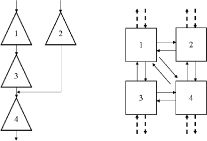
Figure 1: (Left) An example of the traditional reservoir topology assumed in existing works. (Right) An example of a multi-connection reservoir topology considered in this work. Solid lines denote possible transferring directions between two reservoirs. Dashed lines denote natural inflow and released water for consumers in each area.

Secondly, while the goal of existing works is to obtain a dynamic policy of water release, our goal here is to have a static long-term demand-supply plan. In a problem of obtaining a dynamic policy, it is assumed that demand is known for each reservoir in each time period. In our problem, demand (of each reservoir in each time period) itself will be optimized. Therefore, our problem can be considered as a prior step needed to be solved before solving a dynamic policy optimization problem. Moreover, in our problem, a risk management is also taken into account as there will be a risk (a severe loss) if natural inflow supply cannot meet the planned supply. More precisely, after achieving a long-term, e.g. year, demand-supply plan, the obtained plan will be declared to consumers such as farmers and industries. Consumers then integrate the declared supply to their year plans. In order to efficiently utilize their available water, they may invest some money, e.g. farmers may buy new cattle. Therefore, to prevent a futile loss of the investment, if real amount of inflow water is less than what is stated in the plan, the government will have to pay an extra cost, here called a risk, of making extra water from somewhere outside the network, e.g. artificial rain, so that the amount of water will be as specified in the plan.

As a problem is high-dimensional and not dynamic, it is inappropriate to apply stochastic dynamic programming (SDP) as in previous works (?, ?, ?, ?, ?, ?, ?). Beside SDP, deterministic and heuristic approaches such as linear programming, quadratic programming, genetic algorithm and simulated annealing have also been previously employed (?, ?, ?, ?, ?, ?, ?). Nevertheless, these approaches do not directly support the use of stochastic information which is fundamental to reservoir network optimization. In these works, the stochastic information is usually implicitly employed. For examples, given a probability distribution of inflow for each reservoir in each time period, the expected value of inflow can be calculated and input to a deterministic (or heuristic) method.

In this paper, we propose to apply the framework of convex programming to solve the problem. The nowadays technology of convex programming is very efficient like least-square and linear programming, and, with some efforts, many non-linear problems can be reduced to convex programming formulations (?). Similar to linear programming, although convex programming is efficient and appropriate to solve the static problem, a direct application of convex programming does not naturally support the use of stochastic information. Here, we present a novel convex programming formulation which is able to directly take the stochastic information into account and yield a reasonable output.

The remaining of the paper is structured as follows. In Section 2, a mathematical formulation of our problem will be given. In Section 3, related frameworks and our framework which is proposed to solved the problem will be explained. After that, experimental results and discussions are provided subsequently.

2 Problem Specification

Our problem specification here is similar to that of ? (?). However, ? considered only a simple network in Figure 1 (left) and did not consider a static plan with risk management. Let $N$ be the number of reservoirs in the network and $T$ be the number of periods considered in the plan, e.g. one year. Let indices $n,m$ run through $1,...,N$ and $t$ through $1,...,T$. At a period of $t$ a reservoir $n$ can transfer some water to another reservoir $m$ with amount

$$0\leq q^{t}_{nm}\leq Q_{nm},$$ (1)

where $Q_{nm}$ is the maximum pumpage capacity in one period between the two reservoirs. There is also a pumpage cost

$$C^{t}_{nm}(q^{t}_{nm}),$$ (2)

where $C^{t}_{nm}(\cdot)$ is a convex and non-decreasing function. Aside from inputs from other reservoirs, each reservoir will also have its natural inflow input,

$$x^{t}_{n}\sim Pr(x^{t}_{n}),$$ (3)

which is a random variable with respect to a known probability distribution $Pr(x^{t}_{n})$. For each month, there is a profit from releasing water to consumers

$$G^{t}_{n}(g^{t}_{n}),$$ (4)

where $G^{t}_{n}(\cdot)$ is a concave and non-decreasing function, and $g^{t}_{n}$ is an amount of released water to consumers. Let $v_{n}^{t}$ be a volume (after transferring $q_{nm}^{t}$ and releasing $g_{n}^{t}$) of each reservoir on each month. There is a maximum volume $M_{n}$ for each reservoir. If $v_{n}^{t}<M_{n}$, according to the traditional rule of conservation, $v_{n}^{t}$ will depend on $g_{n}^{t}$, $x_{n}^{t}$ and $q_{nm}^{t}$. These relations can be concluded by the following state equation of a volume:

$$v_{n}^{t}=\min\left\{M_{n},v_{n}^{t-1}-g_{n}^{t}+x_{n}^{t}+\sum_{m\neq n}q^{t}_{mn}-\sum_{m^{\prime}\neq n}q^{t}_{nm^{\prime}}\right\}.$$ (5)

And the amount of released and transferred water cannot exceed the existing volume; hence,

$$0\leq g^{t}_{n}+\sum_{n}q^{t}_{nm}\leq v^{t-1}_{n}.$$ (6)

As noted by ? (?), Eq. (6) is conservative since we do not include both (uncertain) natural and transferred inflow at period $t$. In the problem, the initial volume of each reservoir $v^{0}_{n}$ has to be specified. Moreover, there are volume constraints at the end of the optimization period:

$$v^{T}_{n}\geq V_{n}.$$ (7)

Notice that, unlike previous works, there are two notions of sending water from a reservoir, i.e. water transfer $q_{nm}^{t}$ and water release $g_{n}^{t}$. In contrast to water release which is for consumption, water transfer between two reservoirs requires some amount of energy for a pumpage. Hence, there is a cost for water transfer, but a profit for water release.

Finally, we take a risk into account. Since the purpose of a long-term plan considered in this paper is to optimize the demand-supply, after obtaining $g_{n}^{t}$ from an optimizer, the resulted $g_{n}^{t}$ will be declared to consumers such as farmers and industries. Hence, $g_{n}^{t}$ will be their target demand (or, a target supply for the government) since consumers will integrate $g_{n}^{t}$ to their long-term plans. In order to efficiently utilize their available water, consumers may invest some money, e.g. farmers may buy new cattle. As a result of a stochastic nature of $x_{n}^{t}$ stated in Eq.(3), realizable amount of release water $\tilde{g}^{t}_{n}$ may different to its target $g_{n}^{t}$. If $\tilde{g}_{n}^{t}<g_{n}^{t}$, there will be a severe extra cost, or a risk, of acquiring extra water, e.g. by using artificial rain, to satisfy the target demand for consumers:

$$R^{t}_{n}\left(g^{t}_{n}-\tilde{g}^{t}_{n}\right)$$ (8)

where $R^{t}_{n}(\cdot)$ is a convex, non-decreasing function and is zero if $\tilde{g}_{n}^{t}\geq g_{n}^{t}$.

The goal of this optimization problem is to maximize a profit (or minimize a loss) subject to all constraints described above where optimized variables are $\left\{q^{t}_{nm},g^{t}_{n}\right\}$.

3 The Proposed Framework

In this section, we provide our convex optimization framework to solve the problem. However, at first, we motivate the necessary of our framework by illustrating the difficulties of using traditional methods to solve the problem.

3.1 The Need of a New Problem Formulation

From the previous section, it can be observed that our optimization problem is similar to traditional problem formulations of dynamic policy optimization; one may temp to think that methods proposed in previous works can be employed to solve our problem as well. The purpose of this subsection is to explain reasons that existing methods are in fact inappropriate for our current problem, and thus a new method is needed.

We begin by considering the most-popular stochastic dynamic programming (SDP) method (?, ?, ?, ?, ?, ?, ?). There are some difficulties to solve the problem by using SDP due to its nature of dynamic closed-loop control. Firstly, since a long-term static plan is our target, all $\left\{q^{t}_{nm},g^{t}_{n}\right\}_{t=1}^{T}$ must be obtained at the beginning period $t=1$. However, for any $t\geq 2$, a policy obtained from SDP will provide us optimal values of $q^{t}_{nm},g^{t}_{n}$ only when the state variables $\{v^{t-1}_{n},v^{t}_{n}\}$, which are not known at $t=1$, are provided (?, Chapter 17). Secondly, the risk defined in Eq. (8) cannot be straightforwardly taken into account since, by its definition, a risk occurs because a decision has to be made before knowing the real situation (i.e. a decision is made before knowing the future values of state variables); nevertheless, a policy obtained from SDP would provide a decision only after the real situation is known (i.e. a decision will be made in the future). These difficulties may be crudely solved by first implementing traditional closed-loop SDP (without the risk) as illustrated in Figure 2, and then employ the Viterbi algorithm (?, Chapter 15) to find the most-likely sequence of $\{q^{t}_{nm},g^{t}_{n}\}$. Therefore, a series of dynamic controls can be converted to a static plan by this hybrid SDP-Viterbi algorithm. To take the risk into account, some algorithms may be used to further hybridize the SDP-Viterbi algorithm. However, this complicated hybrid method of converting sequential dynamic-controls to a static plan with risk management is beyond the scope of this paper.

Objective:
$\underset{\{q_{nm}^{t},g_{n}^{t}\}}{\max}\ \ {\mathbb{E}}_{x}\left[\underset{t,n}{\sum}G^{t}_{n}\left(g^{t}_{n}\right)-\underset{t,n,m}{\sum}C_{nm}^{t}\left(q_{nm}^{t}\right)\right]$

subject to:
$x^{t}_{n}\sim Pr(x^{t}_{n})$
$0\leq q_{nm}^{t}\leq Q_{nm}$
$0\leq g^{t}_{n}+\sum_{n}q^{t}_{nm}\leq v^{t-1}_{n}$
$v_{n}^{t}=\min\left\{M_{n},v_{n}^{t-1}-g_{n}^{t}+x_{n}^{t}+\sum_{m\neq n}q^{t}_{mn}-\sum_{m^{\prime}\neq n}q^{t}_{nm^{\prime}}\right\}.$
$v_{n}^{T}\geq V_{n}$

Figure 2: The traditional SDP formulation of the multi-connection reservoir optimization problem. This formulation cannot take a risk into account and is intractable.

In fact, we note that there are a third difficulty arising when using SDP since the SDP formulation illustrated Figure 2 is not only stochastic and non-linear, but also high-dimensional. The number of variables grows quadratically with respect to $N$ (due to the $q_{nm}^{t}$ variables); thus, dimensions of the problem is relatively much higher than problems considered in previous works. Due to the curse of dimensionality (?, ?, ?) of discretizing the variables, this high-dimensionality actually prevents the use of SDP in general; even the most efficient SDP approximation, the neuro-dynamic programming method (?), known in literatures can cope with problems of only 30 dimensions (?).

Beside SDP, some existing works proposed to apply deterministic and heuristic approaches such as linear programming (LP), quadratic programming (QP), genetic algorithm and simulated annealing for conventional reservoir networks (?, ?, ?, ?, ?, ?, ?, ?). Nevertheless, the most important limitation of these methods is that they cannot directly take the stochastic information and the risk into account. Usually, uncertainty of inflow is ignored, and $x_{n}^{t}$ is simply replaced by a deterministic value such as its mean $\bar{x}_{n}^{t}$. Henceforth, a deterministic approach with these simple deterministic value inputs will be called a traditional (or conventional) deterministic method. Since a heuristic approach does not guarantee an optimal solution, the traditional deterministic approach is the most suitable method among existing approaches for solving the problem considered here.

Finally, we note that in the literatures of convex optimization itself, there is a methodology called robust programming (?, Chapter 4) which indeed can efficiently utilize the stochastic information. Nonetheless, this robust programming is in fact a worst-case optimization method where the worst situation will be solved. Specifically, in our reservoir problem, robust programming will consider the situation where minimum inflow occurs for each reservoir in each time period. This worst case situation indeed rarely occurs, and hence robust programming is also inappropriate for our problem. In the next section, we present a novel convex optimization formulation which can corporate the stochastic information in a more-efficient way.

3.2 Convex Programming Formulation

Here, we give a new optimization formulation to appropriately solve the problem stated in Section 2 using the convex programming framework (?). Note that in contrast to stochastic dynamic programs, high-dimensional convex programs which are deterministic can be solved efficiently. Moreover, the long-term plan where $\left\{q^{t}_{nm},g^{t}_{n}\right\}_{t=1}^{T}$ is needed at the beginning period can be easily achieved.

The most important step here is to take the stochastic inflow information into this deterministic framework. Our main idea is, instead of treating stochastic inflow variables as random variables or constants like previous works, the stochastic variables $x_{n}^{t}$ themselves will be optimized, as our “best predictions” of inflows. Then, in order to take the risk into account, we propose to consider the average risk of Eq.(8) over all possible actual inflow. The best inflow predictions will be optimized so that they will balance between profits and risks. For instances, if the risk function $R(\cdot)$ is severe, the best predictions will be conservative such that they will smaller than the mean, i.e. $x^{t}_{n}<\bar{x}^{t}_{n}$; this small-value prediction of $x^{t}_{n}$ will limit a predicted volume $v^{t}_{n}$, and hence also limit amount of water transfer $q^{t}_{nm}$, i.e., if the risk is costly and we are unsure of being have abundant of water, we should not transfer the water to other reservoir carelessly; in contrast, if $R(\cdot)$ return low values, the best predictions will be aggressive such that they will be smaller than the mean, i.e. $x^{t}_{n}>\bar{x}^{t}_{n}$.

To formally explain our framework, we first note that if we are able to guarantee that for each reservoir and each time period $v^{t}_{n}\leq M_{n}$, then the state equation simplifies to

$${v}^{t}_{n}={v}_{n}^{t-1}-{g}_{n}^{t}+\tilde{x}_{n}^{t}+\sum_{m\neq n}q^{t}_{mn}-\sum_{m^{\prime}\neq n}q^{t}_{nm^{\prime}}.$$ (9)

It will be explained below that our problem formulation guarantees to satisfy the condition $v^{t}_{n}\leq M_{n}$. Now, suppose an actual (future observed) inflow is $\tilde{x}_{n}^{t}$. Define $\tilde{g}^{t}_{n}$ as the realizable amount of water released by a reservoir $n$ at a period $t$ (see Eq.(8))

$$\tilde{g}^{t}_{n}=g^{t}_{n}+\tilde{v}^{t-1}_{n}-v^{t-1}_{n},$$ (10)

where $\tilde{v}^{t}_{n}$ is as an actual volume defined recursively as

$$\tilde{v}^{t}_{n}=\tilde{v}_{n}^{t-1}-\tilde{g}_{n}^{t}+\tilde{x}_{n}^{t}+\sum_{m\neq n}q^{t}_{mn}-\sum_{m^{\prime}\neq n}q^{t}_{nm^{\prime}},$$ (11)

and $\tilde{v}_{n}^{0}=v_{n}^{0}$. Eq.(10) states that the realizable amount of release from the reservoir $n$ at period $t$ is the target release $g^{t}_{n}$ plus the difference between the actual and target volumes $\tilde{v}^{t-1}_{n}-v^{t-1}_{n}$. By Eq.(10), we have that $\tilde{g}^{t}_{n}-g^{t}_{n}=\tilde{v}^{t-1}_{n}-v^{t-1}_{n}$ and $\tilde{v}^{t-1}_{n}-\tilde{g}^{t}_{n}=v^{t-1}_{n}-g^{t}_{n}$. Using these relations and subtract Eq.(11) with Eq.(9), then, the expected risk ${\mathbb{E}}_{\tilde{x}}\left[R^{t}_{n}\left(g^{t}_{n}-\tilde{g}^{t}_{n}\right)\right]$ can be stated as

$${\mathbb{E}}_{\tilde{x}}\left[R^{t}_{n}\left(g^{t}_{n}-\tilde{g}^{t}_{n}\right)\right]={\mathbb{E}}_{\tilde{x}}\left[R^{t}_{n}\left(x^{t-1}_{n}-\tilde{x}^{t-1}_{n}\right)\right].$$ (12)

For any $t$, to (approximately) calculate ${\mathbb{E}}_{\tilde{x}}\left[R^{t}_{n}\left(x^{t}_{n}-\tilde{x}^{t}_{n}\right)\right]$, we discretize the domain of $Pr(x_{n}^{t})$ into a finite domain set, ${\mathcal{X}}_{n}^{t}$:

$${\mathbb{E}}_{\tilde{x}}\left[R^{t}_{n}\left(x^{t}_{n}-\tilde{x}^{t}_{n}\right)\right]\approx\sum_{\tilde{x}_{n}^{t}\in{\mathcal{X}}_{n}^{t}}Pr(\tilde{x}_{n}^{t})R^{t}_{n}\left(x^{t}_{n}-\tilde{x}^{t}_{n}\right).$$ (13)

Note that in practice the domain of $Pr(x_{n}^{t})$ is originally discrete since we are able to collect only finite statistics of $x_{n}^{t}$ and thus Eq.(13) can be actually exact. Note further that since $R^{t}_{n}(\cdot)$ is convex, $\sum_{\tilde{x}_{n}^{t}\in{\mathcal{X}}}Pr(\tilde{x}_{n}^{t})R^{t}_{n}\left(x^{t}_{n}-\tilde{x}^{t}_{n}\right)$ is also convex.

Objective:
$\underset{\{q_{nm}^{t},g_{n}^{t},x_{n}^{t}\}}{\max}\ \ \underset{t,n}{\sum}{G}_{n}^{t}\left(g_{n}^{t}\right)-\underset{t,n,m}{\sum}C_{nm}^{t}\left(q_{nm}^{t}\right)-\underset{t,n}{\sum}F_{n}^{t}\max\left(v_{n}^{t}-M_{n},0\right)-\underset{t,n}{\sum}{\mathbb{E}}_{\tilde{x}}\left[R^{t}_{n}\left(x^{t}_{n}-\tilde{x}^{t}_{n}\right)\right]$

subject to:
$0\leq q_{nm}^{t}\leq Q_{nm}$
$0\leq g^{t}_{n}+\sum_{n}q^{t}_{nm}\leq v^{t-1}_{n}$
$v_{n}^{t}=v_{n}^{t-1}-g_{n}^{t}+x_{n}^{t}+\sum_{m\neq n}q_{mn}^{t}-\sum_{m^{\prime}\neq n}q_{nm^{\prime}}^{t}$
$v_{n}^{T}\geq V_{n}$
$\min({\mathcal{X}}_{n}^{t})\leq x_{n}^{t}\leq\max({\mathcal{X}}_{n}^{t})$

Figure 3: Summary of the proposed optimization problem.

Our optimization formulation is summarized in Figure 3. This maximization problem formulation consists of a concave objective function and linear constraints, and thus the problem can be efficiently solved by the convex programming framework (?). The initial values of $v_{n}^{0}$ has to be provided.

Note that in order to make our problem formulation convex and efficient, some constraints in Section 2 are changed and new constraints are added. First, the constraint $``\min({\mathcal{X}}_{n}^{t})\leq x_{n}^{t}\leq\max({\mathcal{X}}_{n}^{t})"$ is added so that $x_{n}^{t}$ will take only realizable values. Next, the constraint of Eq.(5) is simplified by introducing a new cost term “$F_{n}^{t}\max(v_{n}^{t}-M_{n},0)$”. Here, $F_{n}^{t}$ is a big constant, and by setting $F_{n}^{t}$ large enough, this will guarantee that $v_{n}^{t}\leq M_{n}$. Note that to obtain a standard objective function form, this term can be easily replaced by a slack variable.

Table 1 summarizes the differences between our framework and the other frameworks. In the table, we do not consider heuristic methods such as genetic algorithm or simulated annealing. The features of heuristic methods are similar to those of deterministic methods: the major difference is that heuristic methods can handle non-linear objective functions. Nevertheless, an ability to handle a non-linear function comes up with a certain tradeoff: heuristic approaches are either sub-optimal or intractable. Also heuristic methods usually were tested with problems with convex objective functions (?, ?, ?, ?). Therefore, our framework presented here can substitute these works with the main advantage that our framework guarantees to find an optimal solution with a polynomial running time. We note also that our framework in fact generalizes traditional uses of LP and QP: if we specify the $Pr(x_{n}^{t}=x^{\prime})=1$ for some $x^{\prime}$ (such as $\bar{x}_{n}^{t}$), then by the constraint $\min({\mathcal{X}}_{n}^{t})<=x_{n}^{t}<=\max({\mathcal{X}}_{n}^{t})$, the best prediction will be $x^{\prime}$, and the risk term $R(x_{n}^{t}-\tilde{x}_{n}^{t})$ will become a constant and can be removed from the optimization problem; for example, in cases that $G(\cdot)$ and $C(\cdot)$ are linearizable, the resulted program is simply an instance of traditional LP applied to a multi-connection reservoir network, see e.g. ? (?).

Table 1: Summary of differences between the three frameworks.

	Traditional SDP	Traditional LP/QP	Our Convex Program
Type	Closed-Loop Control	Open-Loop Optimization	Open-Loop Optimization
Policy	Dynamic: Real-Time Decision	Static: Long-Term Plan	Static: Long-Term Plan
Running Time	Intractable	Tractable	Tractable
Stochastic	Included	Not Included	Included
Objective	Non-linear	Linear/Quadratic	Concave (Maximization)
Risk	Not Included	Not Included	Included
Solution	Sub-Optimal	Optimal	Optimal
$x_{n}^{t}$	Random Variables	Constants	Optimized Variables
$g_{n}^{t}$	Control Variables	Optimized Variables	Optimized Variables
$q_{nm}^{t}$	Control Variables	Optimized Variables	Optimized Variables

4 Experiments

As demonstrated in the previous section (see also Table 1), a deterministic method is the most appropriate candidate among existing methods which can be implemented to solve our problem; hence, in this section, we evaluate our method and compare it to a standard deterministic method. matlab with the optimization interfaces from Yalmip (?) is used for all implementations. For each simulated situation, the following process is employed:

1. All functions, $C_{n}^{t}(\cdot)$, $G_{n}^{t}(\cdot)$ and $R_{n}^{t}(\cdot)$, all constants, $Q_{nm}$ and $M_{n}$, and all probability distributions $Pr(x_{n}^{t})$ are input to our method (or a deterministic method). The long-term demand-supply plan of $\{q_{nm}^{t},g_{n}^{t}\}$ is then obtained for each method.

2. A sequence of inflow is generated $\{\tilde{x}^{t}_{n}\}$ where each $\tilde{x}^{t}_{n}\sim Pr(x^{t}_{n})$. $\{\tilde{g}^{t}_{n}\}$ is then calculated according to Eq.(10) and Eq.(11).

3. The total profit of each method will calculated from:

$$\underset{n}{\sum}G^{t}_{n}\left(g^{t}_{n}\right)-\underset{n,m}{\sum}C_{nm}^{t}\left(q_{nm}^{t}\right)-\underset{n}{\sum}R^{t}_{n}\left(\tilde{g}^{t}_{n}-g^{t}_{n}\right).$$

4. Steps 2. and 3. are repeated 100 times to calculate the average performance of each algorithm.

4.1 Simple Network

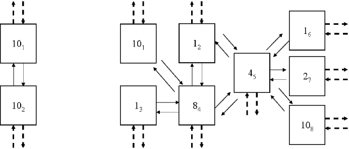
Figure 4: (Left) A simple 2-reservoir network. (Right) The Ang-Puang multi-connection reservoir network being constructed in Petchburi province, Thailand. The maximum volume of each reservoir is indicated. Subscripts denote orders of reservoirs.

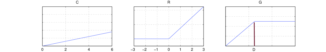
Figure 5: The $C_{n}^{t}(\cdot)$, $R_{n}^{t}(\cdot)$ and $G_{n}^{t}(\cdot)$ employed in the Section 4.1 and Section 4.2.

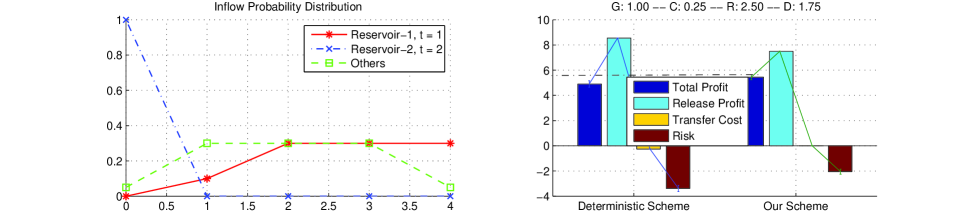
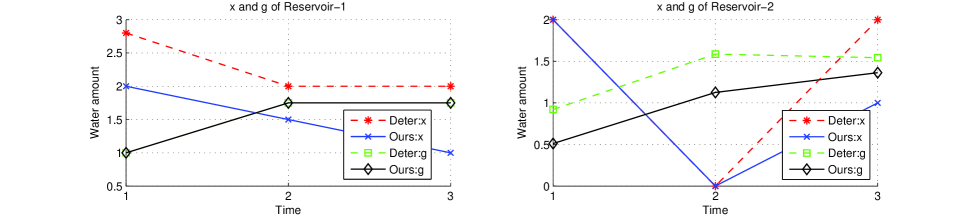
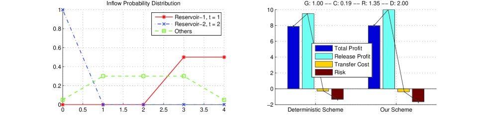
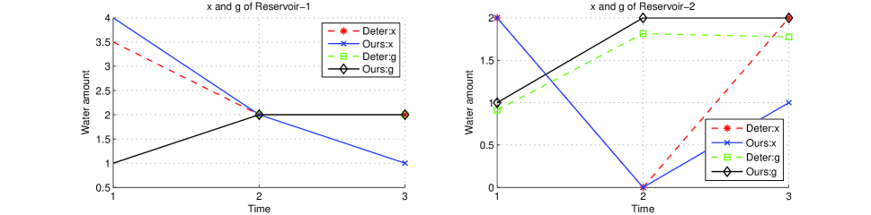
Figure 6: [The Top 4 Figures]: (Up-Left) The probability distributions of inflow used in the simple network. With the exception of $Pr(x_{1}^{1})$ and $Pr(x_{2}^{2})$, the distributions are the same for all $n$ and $t$. (Up-Right) Performance summary: “(Average) Total Profit = Release Profit - Transfer Cost - (Average) Risk” with standard deviations of “Total Profit” and “Risk”. The C,R,G slopes and the D value of Figure 5 are also shown on the top. (Down) $\{x^{t}_{n}\}$ and $\{g^{t}_{n}\}$ are shown for each reservoir. [The Bottom 4 Figures]: Another case of the the simple network.

To intuitively understand results obtained from each algorithm, it is best to start from a a simple reservoir network as illustrated in Figure 4 (Left). Here, $C_{n}^{t}(\cdot)$, $R_{n}^{t}(\cdot)$ and $G_{n}^{t}(\cdot)$ are illustrated in Figure 5 where several values of their slopes and ‘$D$’ (shown in the figure of $G_{n}^{t}(\cdot)$) will be tested. ‘$D$’ can be interpreted as the “maximum demand” for each reservoir at a certain period. In this experiment, these functions are the same for all $n$ and $t$. Since these functions are linearizable, a deterministic method considered in this example is LP. The following values are specified: $T=3$, $N=2$, $M_{1}=M_{2}=10$, $Q_{12}=Q_{21}=5$, and $v^{0}_{1}=v^{0}_{2}=V_{1}=V_{2}=1$. Figure 6 illustrates two cases of this simple network and the corresponding results obtained from traditional LP and our method. The traditional LP implementation can be achieved by simply replacing each uncertain $x_{n}^{t}$ with a deterministic value; $\bar{x}_{n}^{t}$ is used here.

The two cases here illustrate the same simple situation which can be intuitively explained as follows. The first reservoir has a good probability to have more than usual inflow at $t=1$, and the second reservoir will surely do not have any inflow at $t=2$. Therefore, clearly, the first reservoir should send water to the second reservoir on the second period, but the question is: how much should be transferred? The results obtained from traditional and our methods can be used as answers to this question. From the simulations of these two cases (and other several cases not shown here due to the space limitation), our method always significantly outperforms traditional LP. The main reason is because traditional LP inefficiently takes stochastic information into account.

The top 4 figures of Figure 6 illustrate a case where the risk cost is high, and our method becomes more conservative about its predictions of inflow. Even though our method cannot make a high average released profit as that of traditional LP, our method does provide a much lower average risk cost, and therefore results in a higher average total profit (5.49) than that of traditional LP (4.91). The bottom 4 figures of Figure 6 illustrate a second case where a risk plus a transferred cost is not severe and, with high probability, $x_{1}^{1}$ will be very high. In this case, our method results in aggressive inflow prediction of $x^{1}_{1}$ which in turn leads to a higher release profit and a higher average total profit (7.99) compared to that of traditional LP (7.88).

4.2 Complex Network

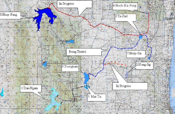
Figure 7: The geography of the Ang-Puang multi-connection reservoir network. “In Progress” denotes a pipe which is being constructed or is planned to be constructed.

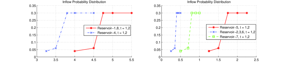
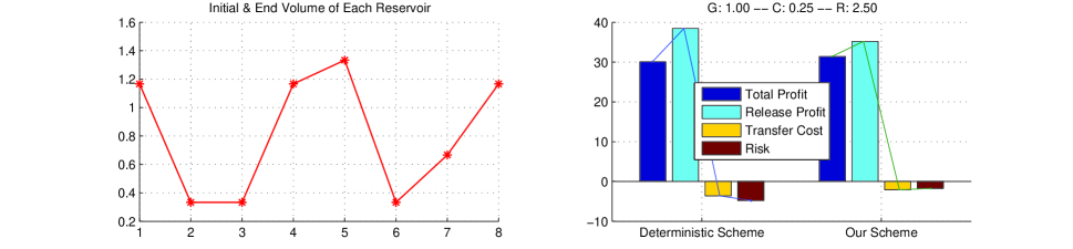
Figure 8: (Up-Left) Inflow probability distributions of the three big reservoirs for $t=1,2$. (Up-Right) Inflow probability distributions of the other reservoirs for $t=1,2$. (Down-Left) $v_{0}$ and $V_{n}$ for each reservoir. (Down-Right) Summary of the profit for each method.

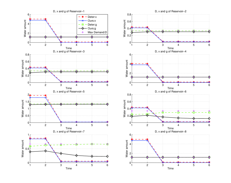
Figure 9: Inflow prediction $x_{n}^{t}$, released volume $g_{n}^{t}$, and $D^{t}_{n}$, for each method and for each reservoir.

Currently, by royal initiating of his Majesty the King of Thailand, a multi-connection reservoir network, namely Ang-Puang, has been being constructed in Petchburi province, Thailand. The geography of the network is shown in Figure 7, and the network topology, together with the capacity of each reservoir (in metric tonne), is shown in Figure 4 (Right). For simplicity, we will mention each reservoir by its order number, e.g. reservoir-1, reservoir-2, etc., instead of its name. Since the network is currently being constructed and all the historical data are being collected, in this experiment we are able to employ only artificial data. The artificial data employed here is in the same spirit as the standard 4 and 10 reservoir problems for a traditional network (?, ?, ?, ?, ?). Nevertheless, our artificial data contains also stochastic information while there is none in the 4 and 10 reservoir problems. Here, $C_{n}^{t}(\cdot)$, $R_{n}^{t}(\cdot)$ and $G_{n}^{t}(\cdot)$ are the same as the previous case, illustrated in Figure 5. The following values are specified: $T=6$, $N=8$, $Q_{nm}=2.5$, $G_{n}^{t}=1$, $C_{nm}^{t}=0.25$ and $R_{n}^{t}=2.5$ for all $n,m,t$. Other parameters are shown in Figure 8 and Figure 9, i.e. Figure 8 illustrates $Pr(x^{t}_{n})$ for $t=1,2$ and $v^{0}_{1}=v^{0}_{2}=V_{1}=V_{2}$, and Figure 9 shows the values of “maximum demand” $D$ specified in $G_{n}^{t}(\cdot)$ for each reservoir in each period.

This problem setting is a simplified version of a real situation normally occured in Thailand where $t$ is a two-month period and $1,...,T$ is thus one year. A long-term plan is determined just before the rainy season; thus, only for $t=1,2$ where $x^{t}_{n}$ will have probabilities to be significantly more than zero, and almost zero in the $t=3,...,6$ periods. To save space, $Pr(x^{t}_{n})$ for $t=3,...,6$ (which their realizable values are around zeros) are not shown. The intuition of this problem setting is that, at the first two periods $t=1,2$, because of the huge amount of rain, all reservoirs will, with high probability, nearly attain their maximum capacities. However, only the big reservoirs $n=1,4,8$ will have enough water for later periods and are responsible to transfer water to the other small reservoirs.

The total profit of the two methods are shown in Figure 8 (Down-Right). Note that, for both methods, standard deviations are almost zeros, and thus our method significantly provides more profit than the conventional deterministic method. As can be seen from Figure 9, in this situation, our method usually becomes more conservative about amount of inflow than the conventional method. As a result, our method cannot guarantee water supply in reservoir-6 and reservoir-7; in contrast, the plan of conventional LP decide to provide almost enough water for every reservoir in every period. Nevertheless, there are often cases that the real inflow $\tilde{x}^{t}_{n}$ for each reservoir is not as high as expected from $x^{t}_{n}$ of the plan of conventional LP; thus, a high risk cost has often to be paid for extra water requirement.

It is also important to note that, in the simulations, the time-complexity of our method increases only slightly from traditional LP. By using matlab’s “linprog” function with the “largescale” option. Our method converges in 18 iterations (4.52 seconds) where traditional LP converges in 17 iterations (4.28 seconds).

4.3 Sensitivity Analysis

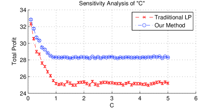
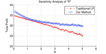
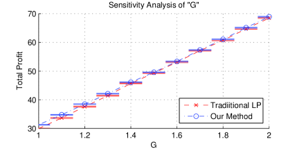
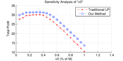
Figure 10: Sensitivity analysis of the two methods.

In this section, we demonstrate the sensitivity of each method with respect to four parameters of the complex-network problem explained in Section 4.2. Figure 10 shows results of the sensitivity analyzes. In each analysis, all the parameters are the same as those of the experiment in Section 4.2, except the analyzed parameter written in the title of each figure. Each figure shows the average total profit of each method in each parameter setting. The standard deviation of the average is also drawn; nevertheless, the standard deviation of each point is very small and is difficult to observe in every figure. This indicates that the statistical confidences of the results shown here are very high. Note that our method always significantly outperforms the existing method in all cases.

Figure 10 (Up-Left) illustrates the case where the parameter ‘$C_{nm}^{t}$’ is varied. We can see that in the beginning where $C_{nm}^{t}\leq 1$, the total profits of the two methods decrease about linearly with respect to the increase of $C_{nm}^{t}$. After $C_{nm}^{t}\geq 1$, the total profits do not change further since the transfer cost becomes more than the release profit $G_{nm}^{t}$, and thus no water transfer occurs after $C_{nm}^{t}>1$.

Figure 10 (Up-Right) illustrates the case where the parameter ‘$R_{n}^{t}$’ is varied. We can see that the average total profit of traditional LP decreases about linearly with respect to the increase of $R_{n}^{t}$. In contrast, the average total profit of our method decreases in a slower rate. This is because our method is able to efficiently take the risk and the stochastic information into account while traditional LP cannot. As a result, our method is less sensitive to the change of $R_{n}^{t}$ than traditional LP.

Figure 10 (Down-Left) illustrates the case where the parameter ‘$G_{n}^{t}$’ is varied. In this case, the average total profits of the two methods increase about linearly with respect to $G_{n}^{t}$. In this case, like other cases, our method provides significantly higher total profit than traditional LP although it is difficult to see in the figure due to the large scale of the y-axis.

Figure 10 (Down-Right) illustrates the case where the parameter ‘$v_{n}^{0}=V_{n}$’ is varied for each reservoir. In this case, the $v_{n}^{0}$ is varied from 5% of $M_{n}$ to 100% of $M_{n}$. As a result, the sensitivity of each method is about the same. Note that as the value of $v_{n}^{0}=V_{n}$ becomes near $M_{n}$, the total profits decrease since the constraint $v_{n}^{T}\geq V_{n}$ forces the optimizer not to use any water at later periods.

5 Discussions

As we explained earlier, a deterministic method seems to be the most appropriate among previously existing methods for the problem of demand-supply optimization in a multi-connection network considered in this paper. From the experiments, we have shown that our new optimization framework gives promising results by always outperforming the existing deterministic method in all experiment settings.

There are some issues which should be considered in practical uses of our method. Firstly, remember that our method requires to discretize $Pr(x_{n}^{t})$. This discretization is not an important limitation of our method since, in practice, all statistics from historical data are in fact originally discrete. Hence, the original statistical distributions can be applied to our method directly. Nevertheless, an application of a smoothing method might be useful to obtain simplified probability distributions which can reduce an optimization time of our method.

Secondly, we note that although the class of convex programming is efficiently solvable, the class of linear programming is still the most preference in term of time efficiency. In fact, theoretically, a convex function can be linearized which an arbitrary degree of approximation accuracy. Therefore, in our opinion, one potential future research direction is to apply an efficient linearization method from the computer vision community to linearize a convex objective function (?, ?), and find the best tradeoff between the time efficiency and the approximation accuracy.

Finally, it is important to note that although our method provides a static long-term plan, our method can be used to dynamically update a plan as well (by re-running the method in the beginning of each time period), provided that the length of $t$ is not shorter than a running time of our method. In all experiments mentioned in Section 4, the optimization process of our method usually accomplished within 1 minute; therefore, for any long-period plans, e.g. $t$ is a week or a month, our method can also provide a dynamic plan.

Acknowledgements

This work was accomplished while the first author stayed at Kanda Laboratory, Ookayama Campus, Tokyo Institute of Technology, and was supported by Japan Student Services Organization (JASSO) under the JENESYS program. We are grateful to Prof. Manabu Kanda and Prof. Kumiko Yokoi for hosting the first author while he was doing this research. We also thank Makoto Nakayoshi and Dr. Kanlaya Sunthornwongsakul for helpful discussions.

References

- Archibald et al. Archibald, T., McKinnon, K., and Thomas, L. (1997). An aggregate stochastic dynamic programming model of multireservoir systems. Water Resources Research, 33(2), 333–340.
- Bellman Bellman, R. (1954). Some problems in the theory of dynamic programming. Econometrica, 37–48.
- Bertsekas and Tsitsiklis Bertsekas, D., and Tsitsiklis, J. (1996). Neuro-dynamic programming. Athena Scientific.
- Boyd and Vandenberghe Boyd, S., and Vandenberghe, L. (2004). Convex Optimization. Cambridge University Press.
- Cai et al. Cai, X., Mckinney, D., and Lasdon, L. (2001). Solving nonlinear water management models using a combined genetic algorithm and linear programming approach. Advances in Water Resources, 24(6), 667–676.
- Castelletti et al. Castelletti, A., De Rigo, D., Rizzoli, A., Soncini-Sessa, R., and Weber, E. (2007). Neuro-dynamic programming for designing water reservoir network management policies. Control Engineering Practice, 15(8), 1031–1038.
- Cervellera et al. Cervellera, C., Chen, V., and Wen, A. (2006). Optimization of a large-scale water reservoir network by stochastic dynamic programming with efficient state space discretization. European Journal of Operational Research, 171(3), 1139–1151.
- Jalali et al. Jalali, M., Afshar, A., and Mariño, M. (2007). Multi-colony ant algorithm for continuous multi-reservoir operation optimization problem. Water Resources Management, 21(9), 1429–1447.
- Kolesnikov and Franti Kolesnikov, A., and Franti, P. (2003). Reduced-search dynamic programming for approximation of polygonal curves. Pattern Recognition Letters, 24(14), 2243–2254.
- Labadie Labadie, J. (2004). Optimal operation of multireservoir systems: State-of-the-art review. Journal of Water Resources Planning and Management, 130(2), 93–111.
- Larson Larson, R. (1968). State increment dynamic programming. Elsevier.
- Li and Wei Li, X., and Wei, X. (2008). An Improved Genetic Algorithm-Simulated Annealing Hybrid Algorithm for the Optimization of Multiple Reservoirs. Water Resources Management, 22(8), 1031–1049.
- Loefberg Loefberg, J. (2004). Yalmip : A toolbox for modeling and optimization in MATLAB. In Proceedings of the CACSD Conference, Taipei, Taiwan.
- Murray and Yakowitz Murray, D., and Yakowitz, S. (1979). Constrained differential dynamic programming and its application to multireservoir control. Water Resources Research, 15, 1017–1027.
- Reis et al. Reis, L., Bessler, F., Walters, G., and Savic, D. (2006). Water Supply Reservoir Operation by Combined Genetic Algorithm–Linear Programming (GA-LP) Approach. Water Resources Management, 20(2), 227–255.
- Russell and Norvig Russell, S., and Norvig, P. (2003). Artificial Intelligence: A Modern Approach, 2 Edition. Prentice Hall.
- Salotti Salotti, M. (2001). An efficient algorithm for the optimal polygonal approximation of digitized curves. Pattern Recognition Letters, 22(2), 215–221.
- Tospornsampan et al. Tospornsampan, J., Kita, I., Ishii, M., and Kitamura, Y. (2005). Optimization of a multiple reservoir system using a simulated annealing–A case study in the Mae Klong system, Thailand. Paddy and Water Environment, 3(3), 137–147.
- Wardlaw and Sharif Wardlaw, R., and Sharif, M. (1999). Evaluation of genetic algorithms for optimal reservoir system operation. Journal of Water Resources Planning and Management, 125(1), 25–33.
- Wurbs Wurbs, R. (1993). Reservoir-system simulation and optimization models. Journal of Water Resources Planning and Management, 119(4), 455–472.
- Wurbs Wurbs, R. (2005). Comparative evaluation of generalized river/reservoir system models. Civil Engineering Department, Texas A&M University.
- Yakowitz Yakowitz, S. (1982). Dynamic programming applications in water resources. Water Resources Research, 18(4).