A universal form of slow dynamics in zero-temperature random-field Ising model

Abstract

The zero-temperature Glauber dynamics of the random-field Ising model describes various ubiquitous phenomena such as avalanches, hysteresis, and related critical phenomena. Here, for a model on a random graph with a special initial condition, we derive exactly an evolution equation for an order parameter. Through a bifurcation analysis of the obtained equation, we reveal a new class of cooperative slow dynamics with the determination of critical exponents.

Slow dynamical behaviors caused by cooperative phenomena are observed in various many-body systems. In addition to well-studied examples such as critical slowing down H-H , phase ordering kinetics Bray , and slow relaxation in glassy systems Cavagna , seemingly different phenomena from these examples have also been discovered successively. In order to judge whether or not an observed phenomenon is qualitatively new, one needs to determine a universality class including the phenomenon. In this context, it is significant to develop a theoretical method for classifying slow dynamics.

Here, let us recall a standard procedure for classifying equilibrium critical phenomena. First, for an order parameter $m$ of a mean-field model, a qualitative change in the solutions of a self-consistent equation $m={\cal F}(m)$ is investigated; then, the differences between the results of the mean-field model and finite-dimensional systems are studied by, for example, a renormalization group method. On the basis of this success, an analysis of the dynamics of a typical mean-field model is expected to be a first step toward determining a universality class of slow dynamics.

As an example, in the fully connected Ising model with Glauber dynamics, an evolution equation for the magnetization, $\partial_{t}m={\cal G}(m)$, can be derived exactly. The analysis of this equation reveals that the critical behavior is described by a pitchfork bifurcation in the dynamical system theory Gucken . As another example, an evolution equation for a time-correlation function and a response function was derived exactly for the fully connected spherical $p$-spin glass model CHZ ; Kurchan . The obtained evolution equation represents one universality class related to dynamical glass transitions.

The main purpose of this Letter is to present a non-trivial class of slow dynamics by exactly deriving an evolution equation for an order parameter. The model that we consider is the zero-temperature Glauber dynamics of a random-field Ising model, which is a simple model for describing various ubiquitous phenomena such as avalanches, hysteresis, and related critical phenomena Inomata ; Sethna ; Vives ; Durin ; Shin1 . As a simple, but still non-trivial case, we analyze the model on a random graph fn:global , which is regarded as one type of Bethe lattices MP . Thus far, several interesting results on the quasi-static properties of the model on Bethe lattices have been obtained Duxbury1 ; Illa ; Dhar1 ; Colaiori1 ; Alava ; Rosinberg0 ; Rosinberg1 . In this Letter, by performing the bifurcation analysis of the derived equation, we determine the critical exponents characterizing singular behaviors of dynamical processes.

Model:

Let $G(c,N)$ be a regular random graph consisting of $N$ sites, where each site is connected to $c$ sites chosen randomly. For a spin variable $\sigma_{i}=\pm 1$ and a random field $h_{i}^{\prime}$ on the graph $G(c,N)$, the random-field Ising model is defined by the Hamiltonian

$$H=-\frac{1}{2}\sum_{i=1}^{N}\sum_{j\in B_{i}}\sigma_{i}\sigma_{j}-\sum_{i=1}^{N}(h+{h}_{i}^{\prime})\sigma_{i},$$ (1)

where $B_{i}$ represents a set of sites connected to the $i$ site and $h$ is a uniform external field. The random field ${h}_{i}^{\prime}$ obeys a Gaussian distribution $D_{R}({h}_{i}^{\prime})$ with variance $R$. We collectively denote $(\sigma_{i})_{i=1}^{N}$ and $(h_{i})_{i=1}^{N}$ by ${\boldsymbol{\sigma}}$ and ${\boldsymbol{h}}$, respectively. Let $u_{i}$ be the number of upward spins in $B_{i}$. Then, for a given configuration, we express the energy increment for the spin flip at $i$ site as $-2\sigma_{i}\Delta_{i}$, where

$$\Delta_{i}\equiv c-2u_{i}-(h+{h}_{i}^{\prime}).$$ (2)

The zero-temperature Glauber dynamics is defined as a stochastic process in the limit that the temperature tends to zero for a standard Glauber dynamics with a finite temperature. Specifically, we study a case in which the initial condition is given by $\sigma_{i}=-1$ for any $i$. In this case, once $\sigma_{i}$ becomes positive, it never returns. Thus, the time evolution rule is expressed by the following simple rule: if $\sigma_{i}=-1$ and $u_{i}$ satisfies $\Delta_{i}\leq 0$, the spin flips at the rate of $1/\tau_{0}$; otherwise, the transition is forbidden. Note that $\sigma_{i}(t)=-1$ when $\Delta_{i}(t)>0$, and $\Delta_{i}(t)$ is a non-increasing function of $t$ in each sample Dhar1 . In the argument below, a probability induced by the probability measure for the stochastic time evolution for a given realization ${\boldsymbol{h}}$ is denoted by $P^{{\boldsymbol{h}}}$, and the average of a quantity $X$ over ${\boldsymbol{h}}$ is represented by $\overline{X}$.

Order parameter equation:

We first note that the local structure of a random graph is the same as a Cayley tree. In contrast to the case of Cayley trees, a random graph is statistically homogeneous, which simplifies the theoretical analysis. Furthermore, when analyzing the model on a random graph in the limit $N\to\infty$, we may ignore effects of loops. Even with this assumption, the theoretical analysis of dynamical behaviors is not straightforward, because $\sigma_{j}$ and $\sigma_{k}$, $j,k\in B_{i}$, are generally correlated. We overcome this difficulty by the following three-step approach.

The first step is to consider a modified system in which $\sigma_{i}=-1$ is fixed irrespective of the spin configurations. We denote a probability in this modified system by $Q^{{\boldsymbol{h}}}$. We then define $q(t)\equiv\overline{Q^{{\boldsymbol{h}}}(\sigma_{j}(t)=1)}$ for $j\in B_{i}$, where $q(t)$ is independent of $i$ and $j$ owing to the statistical homogeneity of the random graph. The second step is to confirm the fact that any configurations with $\Delta_{i}(t)>0$ in the original system are realized at time $t$ in the modified system as well, provided that the random field and the history of a process are identical for the two systems. This fact leads to a non-trivial claim that $P^{{\boldsymbol{h}}}(\Delta_{i}(t)>0)$ is equal to $Q^{{\boldsymbol{h}}}(\Delta_{i}(t)>0)$. By utilizing this relation, one may express $P^{{\boldsymbol{h}}}(\Delta_{i}(t)>0)$ in terms of $Q^{{\boldsymbol{h}}}(\sigma_{j}(t)=1)$. The average of this expression over ${\boldsymbol{h}}$, with the definition $\rho(t)\equiv\overline{P^{{\boldsymbol{h}}}(\Delta_{i}(t)>0)}$, leads to

$$\rho(t)=\sum_{u=0}^{c}\left(\begin{array}[]{c}c\\ u\end{array}\right)q(t)^{u}(1-q(t))^{c-u}\int_{-\infty}^{c-2u-h}dh^{\prime}D_{R}(h^{\prime}),$$ (3)

where we have employed the statistical independence of $\sigma_{j}$ and $\sigma_{k}$ with $j,k\in B_{i}$ in the modified system. The expression (3) implies that $q(t)$ defined in the modified system has a one-to-one correspondence with the quantity $\rho(t)$ defined in the original system. The third step is to define $p(t)\equiv\overline{Q^{{\boldsymbol{h}}}(\sigma_{j}=-1,\Delta_{j}\leq 0)}$ and $r(t)\equiv\overline{Q^{{\boldsymbol{h}}}(\Delta_{j}(t)>0)}$ for $j\in B_{i}$. Then, by a procedure similar to the derivation of (3), we find that $dq(t)/dt$ is equal to $p(t)/\tau_{0}$. $r(t)$ is also expressed as a function of $q(t)$ because $r(t)$ is equal to a probability of $\Delta_{j}(t)>0$ in a modified system with $\sigma_{i}=-1$ and $\sigma_{j}=-1$ fixed. Concretely, we write $r(t)=1-F(q(t))$, where

$$F(q)=\sum_{u=0}^{c-1}\left(\begin{array}[]{c}c-1\\ u\end{array}\right)q^{u}(1-q)^{c-1-u}\int_{c-2u-h}^{\infty}dh^{\prime}D_{R}(h^{\prime}).$$ (4)

By combining a trivial relation $p(t)+q(t)+r(t)=1$ with these results, we obtain

$$\tau_{0}\dfrac{dq}{dt}=F(q)-q,$$ (5)

which determines $q(t)$ with the initial condition $q(0)=0$.

Here, for a spin configuration at time $t$ under a quenched random field $h_{i}^{\prime}$, we define

$${\hat{\rho}}(t)\equiv\frac{1}{N}\sum_{i=1}^{N}\theta(\Delta_{i}(t)),$$ (6)

where $\theta(x)=1$ for $x>0$ and $\theta(x)=0$ otherwise. Due to the law of large numbers, ${\hat{\rho}}(t)$ is equal to $\rho(t)$ in the limit $N\to\infty$. Since $\rho(t)$ is determined by (3) with (5), one may numerically compare $\rho(t)$ with ${\hat{\rho}}(t)$ observed in the Monte Calro (MC) simulations. We confirmed that these two results coincided with each other within numerical accuracy. We also numerically checked the validity of (5) on the basis of the definition of $q$. As a further evidence of the validity of our results, we remark that the stationary solution $q(\infty)$ satisfies $q(\infty)=F(q(\infty))$, which is identical to the fixed-point condition of a recursive equation $Z_{n+1}=F(Z_{n})$ in the Cayley tree, where $Z_{n}$ is a probability at generation $n$. (See Ref. Dhar1 for the precise definition of $Z_{n}$.) In the argument below, we set $\tau_{0}=1$ without loss of generality and we investigate the case $c=4$ as an example. The obtained results are essentially the same for $c>4$; however, the behaviors for $c<4$ are qualitatively different from those for $c\geq 4$.

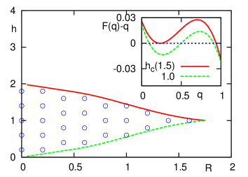
Figure 1: (color online) Phase diagram. Inset: $F(q)-q$ as functions of $q$. $R=1.5$. $h=1.0$ and $h=h_{c}(R)$.

Bifurcation analysis:

We start with the analysis of (5) for $R=1.5$ and $h=1.0$. The qualitative behavior of $q(t)$ is understood from the shape of the graph $F(q)-q$ shown in the inset of Fig. 1. There are three zeros, $q_{1}$, $q_{2}$, and $q_{3}$, where $0<q_{1}<q_{2}<q_{3}<1$. Since $F(q)>q$ in the interval $[0,q_{1})$, $q(t)\to q_{1}$ as $t\to\infty$ with the initial condition $q(0)=0$. This geometrical structure sustains in a region of the parameter space $\alpha\equiv(R,h)$, as shown in Fig. 1. Let $q_{i}(\alpha)$ be the parameter dependence of $q_{i}$. Then, the stable fixed point $q_{1}(\alpha)$ and the unstable fixed point $q_{2}(\alpha)$ merge at the solid line, and the stable fixed point $q_{3}(\alpha)$ and the unstable fixed point $q_{2}(\alpha)$ merge at the dashed line, both of which correspond to saddle-node bifurcations Gucken . The two lines terminate at a critical point $(R_{\rm sp},h_{\rm sp})$. Since the trajectories with the initial condition $q(0)=0$ do not exhibit a singularity at the dashed line, only the bifurcations at the solid line are relevant in the present problem. The solid line is called a spinodal line Dahmen0 .

Now, we investigate the singular behaviors of slow dynamics near the bifurcation points. We first fix the value of $R$ such that $0<R\ll R_{\rm sp}$. Then, a saddle-node bifurcation occurs at $(R,h_{\rm c}(R))$ on the solid line. Let $q_{\rm c}(R)$ be the saddle-node point such that $q_{1}=q_{2}=q_{\rm c}(R)$. We set $h=h_{\rm c}(R)+\epsilon$ and $q=q_{\rm c}+u$. From the graph in the inset of Fig. 1, one finds that (5) becomes

$$\dfrac{du}{dt}=a_{0}\epsilon+a_{2}u^{2}+O(|u|^{3},|\epsilon u|),$$ (7)

when $|u|\ll 1$ and $|\epsilon|\ll 1$. $a_{0}$ and $a_{2}$ are numerical constants. Solutions of (7) are expressed as a scaling form

$$u(t)=|\epsilon|^{1/2}\bar{u}_{\pm}(|\epsilon|^{1/2}t)$$ (8)

when $|\epsilon|\ll 1$, where $\bar{u}_{+}$ and $\bar{u}_{-}$ are $\epsilon$-independent functions for $\epsilon>0$ and $\epsilon<0$, respectively. The result implies that the characteristic time near $q=q_{\rm c}$ diverges as $\tau\simeq|\epsilon|^{-1/2}.$ Note that $q(t\to\infty)=q_{3}$ when $\epsilon>0$. Therefore, $q(t\to\infty)$ exhibits a discontinuous change, and the jump width is given by the distance between $q_{1}(\alpha)=q_{2}(\alpha)$ and $q_{3}(\alpha)$ at $\epsilon=0$.

Next, we focus on the dynamical behaviors near the critical point $(R_{\rm sp},h_{\rm sp})$. By substituting $q=q_{\rm c}(R_{\rm sp})+v$ and $(R,h)=(R_{\rm sp},h_{\rm sp})+(\eta,\epsilon)$ into (5), we obtain

$$\dfrac{dv}{dt}=c_{0}\epsilon+c_{1}\eta v-c_{3}v^{3}+O(|v|^{4},|\epsilon v|,|\eta v^{2}|),$$ (9)

when $|v|\ll 1$, $|\epsilon|\ll 1$, and $|\eta|\ll 1$. $c_{0}$, $c_{1}$, and $c_{3}$ are numerical constants. System behaviors are classified into two types. First, when $|\eta|\gg|\epsilon|^{2/3}$, solutions of (9) are expressed as $v=|\eta|^{1/2}\bar{v}_{1\pm}(|\eta|t)$ when $|\eta|\ll 1$. This scaling form is identical to that near a pitchfork bifurcation, which might be related to conjectures presented in Refs. Perez ; Colaiori2 ; Dahmen1 . Second, when $|\eta|\ll|\epsilon|^{2/3}$, which includes the case in which $R=R_{\rm sp}$ is fixed, solutions of (9) are expressed as

$$v=|\epsilon|^{1/\delta}\bar{v}_{2\pm}(|\epsilon|^{\zeta}t)$$ (10)

when $|\epsilon|\ll 1$, with $\delta=3$ and $\zeta=2/3$. The characteristic time diverges as $\tau\simeq|\epsilon|^{-\zeta}$ near the critical point $(R_{\rm sp},h_{\rm sp})$. In addition to the two scaling forms, one can calculate the width of the discontinuous jump of $q$ along the spinodal line, which is proportional to $(-\eta)^{1/2}$ near the critical point Colaiori1 ; Duxbury1 .

Finite size fluctuations:

In a system with large but finite $N$, fluctuations of $\hat{\rho}$ are observed. Their basic characterization is given by the intensity

$$\chi_{\rho}(t)\equiv N\left\langle({\hat{\rho}}(t)-\left\langle{\hat{\rho}}(t)\right\rangle)^{2}\right\rangle.$$ (11)

where for a quantity $\hat{X}(t)$ determined by ${\boldsymbol{\sigma}}(t)$ and ${\boldsymbol{h}}$, $\left\langle\hat{X}(t)\right\rangle\equiv\overline{\sum_{{\boldsymbol{\sigma}}}P^{{\boldsymbol{h}}}({\boldsymbol{\sigma}}(t)={\boldsymbol{\sigma}})\hat{X}(t)|_{{\boldsymbol{\sigma}}(t)={\boldsymbol{\sigma}}}}$. The problem here is to determine a singular behavior of $\chi_{\rho}$ under the condition that $0<\epsilon\ll 1$ and $\eta=0$. Let $\rho_{\rm c}$ be defined by (3) with $q=q_{\rm c}(R_{\rm sp})$. We then assume

$${\hat{\rho}}(t)-\rho_{\rm c}=A(\epsilon,N)\hat{F}(t/\tau(\epsilon,N))$$ (12)

near ${\hat{\rho}}(t)\simeq\rho_{\rm c}$, where $A$ and $\tau$ are typical values of the amplitude and the characteristic time, respectively, and $\hat{F}$ is a time-dependent fluctuating quantity scaled with $A$ and $\tau$. We further conjecture finite size scaling relations

$$A(\epsilon,N) = N^{-1/(\nu\delta)}F_{A}(\epsilon N^{1/\nu}),$$

$$\tau(\epsilon,N) = N^{\zeta/\nu}F_{\tau}(\epsilon N^{1/\nu}),$$ (13)

where $F_{A}(x)\simeq x^{1/\delta}$ for $x\gg 1$ and $F_{\tau}(x)\simeq x^{-\zeta}$ for $x\gg 1$; $F_{A}(x)={\rm const.}$ and $F_{\tau}(x)={\rm const.}$ for $x\ll 1$. Here, the exponent $\nu$ characterizes a cross-over size $N_{\rm c}$ between the two regimes as a power-law form $N_{\rm c}\simeq\epsilon^{-\nu}$. We thus obtain

$$\chi_{\rho}(\tau(\epsilon,N))=N^{\gamma/\nu}F_{\chi}(\epsilon N^{1/\nu}),$$ (14)

where $\gamma=\nu-2/\delta$. The values of $\zeta$ and $\delta$ have already been determined. We derive the value of $\nu$ in the following paragraph.

It is reasonable to assume that the qualitative behavior of $\hat{\rho}$ near the critical point $(R_{\rm sp},h_{\rm sp})$ is described by (9) with small fluctuation effects due to the finite size nature. There are two types of fluctuation effects: one from the stochastic time evolution and the other from the randomness of $h_{i}^{\prime}$. The former type is expressed by the addition of a weak Gaussian-white noise with a noise intensity proportional to $1/N$, whereas the latter yields a weak quenched disorder of the coefficients of (9). In particular, $\epsilon$ is replaced with $\epsilon+\hat{g}/\sqrt{N}$, where $\hat{g}$ is a time-independent quantity that obeys a Gaussian distribution. Then, two characteristic sizes are defined by a balance between the fluctuation effects and the deterministic driving force. As the influence of the stochastic time evolution rule, the size $N_{\rm s}$ is estimated from a dynamical action of the path-integral expression $\int dt[Nc_{4}(\partial_{t}v-c_{0}\epsilon+c_{3}v^{3})^{2}+c_{5}v^{2}]$, where the last term is a so-called Jacobian term. $c_{4}$ and $c_{5}$ are constants. In fact, the balance among the terms $\epsilon^{2}\simeq v^{6}\simeq v^{2}/N_{\rm s}$ leads to $N_{\rm s}\simeq\epsilon^{-4/3}$. (See Refs. Iwata ; Ohta2 for a similar argument.) On the other hand, the size $N_{\rm q}$ associated with the quenched disorder is determined by the balance $\epsilon\simeq 1/\sqrt{N_{\rm q}}$, which leads to $N_{\rm q}\simeq\epsilon^{-2}$. Since $N_{\rm s}\ll N_{\rm q}$ for $\epsilon\ll 1$, the system is dominated by fluctuations when $N\leq N_{\rm q}$. With this consideration, we conjecture that $N_{\rm c}=N_{\rm q}\simeq\epsilon^{-2}$. That is, $\nu=2$.

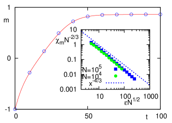
Figure 2: (color online) Time evolution of the magnetization for $R=1.781258(\simeq R_{\rm sp})$ and $h=1.1$. Note that $h_{\rm sp}=1$. The circles are the result obtained by the MC simulations with $N=10^{5}$, and the solid line corresponds to the solution of $\partial_{t}m=-(m-1+2\rho)$ with (3) and (5). One may derive this equation for $m$ in a straightforward manner. Inset: $\chi_{\rm m}N^{-2/3}$ as functions of $\epsilon N^{1/2}$. The guideline represents $\chi_{\rm m}\simeq\epsilon^{-4/3}$.

In laboratory and numerical experiments, statistical quantities related to the magnetization $\hat{m}=\sum_{i=1}^{N}\sigma_{i}/N$ may be measured more easily than $\chi_{\rho}$. Since $\hat{m}$ is not independent of ${\hat{\rho}}$, $\hat{m}$ also exhibits singular behaviors near the critical point. Concretely, the fluctuation intensity $\chi(t)\equiv N\left(\left\langle\hat{m}^{2}(t)\right\rangle-\left\langle\hat{m}(t)\right\rangle^{2}\right)$ is characterized by the above exponents. In order to confirm this claim, we measured $\chi(t)$ by MC simulations. Then, the characteristic time is defined as a time $t_{*}$ when $\chi(t)$ takes a maximum value $\chi_{\rm m}$. Our theory predicts $t_{*}\simeq\epsilon^{-2/3}$ and $\chi_{\rm m}=N^{2/3}\bar{\chi}_{\rm m}(\epsilon N^{1/2})$ with $\bar{\chi}_{\rm m}(x)\simeq x^{-4/3}$ for $x\gg 1$. The numerical results shown in Fig. 2 are consistent with the theoretical predictions.

Concluding remarks:

We have derived the exact evolution equation for the order parameter $\rho$ describing the dynamical behaviors of a random field Ising model on a random graph. From this dynamical system, we have determined the values of the critical exponents: $\zeta=2/3$, $\delta=3$, $\nu=2$, and $\gamma=4/3$.

Before ending this Letter, we discuss the critical phenomena in $d$-dimensional random-field Ising models on the basis of our theoretical results. Let $\nu_{\rm m}$ be the critical exponent characterizing the divergence of a correlation length above an upper-critical dimension $d_{\rm u}$. By assuming a standard diffusion coupling for (9) as an effective description of finite-dimensional systems, we expect $z\equiv\zeta/\nu_{\rm m}=2$. This leads to $\nu_{\rm m}=1/3$. From an application of a hyper-scaling relation to the upper-critical dimension, one also expects the relation $\nu=d_{\rm u}\nu_{\rm m}$ Pfeuty . This leads to $d_{\rm u}=\nu/\nu_{\rm m}=6$, which is consistent with the previous result Dahmen0 . We then denote the exponents characterizing the divergences of time and length scales by $\nu_{3}$ and $\zeta_{3}$, respectively, for three-dimensional systems. These values were estimated as $\zeta_{3}\simeq 1.3$ and $\nu_{3}\simeq 0.7$ in numerical experiments Carpenter ; Perez ; Ohta1 . The theoretical analysis of finite dimensional systems will be attempted as an extension of the present work; this might be complementary to previous studies Dahmen0 ; Muller . Finally, we wish to mention that one of the most stimulating studies is to discover such a universality class in laboratory experiments by means of experimental techniques that capture spatial structures directly Shin1 ; Shin2 ; Durin .

We acknowledge M. L. Rosinberg, G. Semerjian, S. N. Majumdar, H. Tasaki, and G. Tarjus for the related discussions. This work was supported by a grant from the Ministry of Education, Science, Sports and Culture of Japan, Nos. 19540394 and 21015005. One of the authors (H.O.) is supported by a Grant-in-Aid for JSPS Fellows.

References

- (1) P. C. Hohenberg and B. I. Halperin, Rev. Mod. Phys. 49, 435 (1977).
- (2) A. J. Bray, Advances in Physics 43, 357 (1994).
- (3) A. Cavagna, Physics Reports 476, 51 (2009).
- (4) J. Guckenheimer and P. Holmes, Nonlinear Oscillations, Dynamical Systems and Bifurcations of Vector Fields, (Springer-Verlag, New York, 1983).
- (5) A. Crisanti, H. Horner, and H. J. Sommers, Z. Phys. B 92, 257 (1993).
- (6) L. F. Cugliandolo and J. Kurchan, Phys. Rev. Lett. 71, 173 (1993).
- (7) A. Berger, A. Inomata, J. S. Jiang, J. E. Pearson, and S. D. Bader, Phys. Rev. Lett. 85, 4176 (2000).
- (8) J. P. Sethna, K. A. Dahmen, and C. R. Myers, Nature 410, 242 (2001).
- (9) J. Marcos, E. Vives, L. Manosa, M. Acet, E. Duman, M. Morin, V. Novak, and A. Planes, Phys. Rev. B 67, 224406 (2003).
- (10) M. Lobue, V. Basso, G. Beatrice, C. Bertotti, G. Durin, and C. P. Sasso, J. Magn. Mat. 290, 1184 (2005).
- (11) M.-Y. Im, D.-H. Kim, P. Fischer, and S.-C. Shin, Appl. Phys. Lett. 95, 182504 (2009).
- (12) The fully connected model exhibits a qualitatively different behavior from finite dimensional systems Duxbury1 ; Illa .
- (13) M. Mézard and G. Parisi, Eur. Phys. J. B 20, 217 (2001).
- (14) D. Dhar, P. Shukla, and J. P. Sethna, J. Phys. A: Math. Gen. 30, 5259 (1997).
- (15) F. Colaiori, A. Gabrielli, and S. Zapperi, Phys. Rev. B 65, 224404 (2002).
- (16) R. Dobrin, J. H. Meinke, and P. M. Duxbury, J. Phys. A: Math. Gen. 35, 247 (2002).
- (17) M. J. Alava, V. Basso, F. Colaiori, L. Dante, G. Durin, A. Magni, and S. Zapperi, Phys. Rev. B 71, 064423 (2005).
- (18) X. Illa, P. Shukla, and E. Vives, Phys. Rev. B 73, 092414 (2006).
- (19) X. Illa, M. L. Rosinberg, and G. Tarjus, Eur. Phys. J. B 54, 355 (2006).
- (20) M. L. Rosinberg, G. Tarjus, and F. J. Pérez-Reche, J. Stat. Mech. P03003 (2009).
- (21) K. A. Dahmen and J. P. Sethna, Phys. Rev. B 53, 14872 (1996).
- (22) F. J. Pérez-Reche and E. Vives, Phys. Rev. B 67, 134421 (2004).
- (23) F. Colaiori, M. J. Alava, G. Durin, A. Magni, and S. Zapperi, Phys. Rev. Lett. 92, 257203 (2004).
- (24) Y. Liu and K. A. Dahmen, Europhys. Lett. 86, 56003 (2009).
- (25) H. Ohta and S. Sasa, Phys. Rev. E 78, 065101(R) (2008).
- (26) M. Iwata and S. Sasa, J. Phys. A: Math. Gen. 42, 075005 (2009).
- (27) R. Botet, R. Jullien, and P. Pfeuty, Phys. Rev. Lett. 49, 478 (1982).
- (28) J. H. Carpenter and K. A. Dahmen, Phys. Rev. B 67, 020412 (2003).
- (29) H. Ohta and S. Sasa, Phys. Rev. E 77, 021119 (2008).
- (30) M. Müller and A. Silva, Phys. Rev. Lett. 96, 117202 (2006).
- (31) D.-H. Kim, H. Akinaga, and S.-C. Shin, Nature Phys. 3, 547 (2007).