The Influence Of Elastic Deformations On The Supersolid Transition

Abstract

We study, within the Ginzburg-Landau (GL) theory of phase transitions, how elastic deformations in a supersolid lead to local changes in the supersolid transition temperature. The GL theory is mapped onto a Schrödinger-type equation with an effective potential that depends on local dilatory strain. The effective potential is attractive for local contractions and repulsive for local expansion. Different types of elastic deformations are studied. We find that a contraction (expansion) of the medium that may be brought about by, e.g., applied stress leads to a higher (lower) transition temperature as compared to the unstrained medium. In addition, we investigate edge dislocations and illustrate that the local transition temperature may be increased in the immediate vicinity of the dislocation core. Our analysis is not limited to supersolidity. Similar strain effects should also play a role in superconductors.

I Introduction

Superfluids flow without resistance. The existence of superfluidity raised the possibility of supersolids supersolid ; Chester - solids in which superfluidity can occur without disrupting crystalline order. Long ago, Chester Chester theoretically demonstrated the possible existence of a supersolid. If supersolids exist, a natural contender would be solid Helium. Prokof'ev2007 Recent torsional oscillator experiments KC on solid ⁴He pointed to supersolid type features and have led to a flurry of activity. In the simplest explanation of the experiments, KC a portion of the medium becomes, at low temperatures, a superfluid that decouples from the measurement apparatus. Such a “Non Classical Rotational Inertia” (NCRI) effect is known to exist in superfluid liquid Helium London ; Fairbank which was probed with similar techniques. Fairbank ; Andron Experimental results suggest the absence of superfluid features in ideal crystals with no grain boundaries. Sasaki Currently, it is not clear if an NCRI lies at the core of the recent experimental findings in solid ⁴He. For instance, the required condensate fraction adduced from a simple NCRI-only explanation does not simply conform with thermodynamic measurements bgnt . Rittner and Reppy Reppy discovered that the putative super-solid type feature is acutely sensitive to the quench rate for solidifying the liquid. Aoki, Keiderling, and Kojima reported rich hysteresis and memory effects Kojima similar to those occurring in glasses memory . The torsional oscillator findings can arise from material characteristics alone. dynamics ; dorsey ; Huse07 ; DSB ; iw ; andreev ; korshunov ; plastic In particular, the thermodynamics and transient dynamics of distributed processes in amorphous or general non-equilibrated solids can currently fit bgnt ; dynamics observed results. Indeed, later numerical results point towards such a possibility. giuilio Notably, recent experimental results science agree with an earlier suggested theory concerning such transient dynamics. dynamics The presence of non-uniformity in ⁴He is also suggested by a criterion comparing the change in dissipation vs. relative period shift in torsion oscillator. Huse07 It may well be that these glassy and superfluid effects are present in solid Helium. superglass An interesting question concerns the coupling between elastic defects such as dislocations and superfluid type features. znmc The coupling of the supersolid transition to impurities was discussed in Ref. ba, . The coupling between superfluidity and elasticity in supersolids and how this may lead to a strain-dependent critical temperature was discussed in Refs. DGT, ; Toner, . The viable existence of supersolid phase is not confined to solid Helium. Other contenders for the supersolid state include cold atoms in a confining optical lattice. coldatom There has been much work examining supersolidity in spin systems as well, see, for example, Ref. cristian, . Supersolids constitute a fascinating state of matter and appear in a host of systems.

This article focuses on the coupling between nanoscale structure and supersolidity. DGT ; Toner As is well appreciated, elastic strain may fundamentally affect local and mesoscopic electronic, magnetic and structural properties. There is ample evidence for significant coupling amongst the electronic degrees of freedom with the lattice distortions in cuprates, manganites, and ferroelectrics. review-ela ; strain_PRL The central thesis of this work is that elastic distortions may alter the supersolid behavior. As we will elaborate later on, in, e.g., a cylindrical torsional oscillator geometry in which the boundary of the solid is elastically deformed so that it undergoes a supersolid transition at a higher temperature than the bulk, a fraction of the boundary will become a supersolid leading to a partial decoupling of the bulk from the torsional oscillator chassis and a consequent reduction in the period.

In this work, we will employ a Ginzburg-Landau (GL) theory to study the influence of elastic strain on supersolidity. As we will show, the Euler-Lagrange equations for the GL free energy result in an effective Schrödinger type equation. We find the lattice distortion acts as an effective potential for the supersolid order parameter. Solving the resulting effective Schrödinger–type equation, we find our main results: (1) a contraction (expansion) of the lattice edges leads to an increase (decrease) in the local supersolid transition temperature; (2) elastic defects, such as dislocations, lead to similar effects.

Although our motivation is the analysis of supersolids, all of our calculations within the GL framework are identical for non-uniform elastically strained superconductors strain_PRL ; sc1 and lead to the same general conclusions, which we will derive in this work. The case of uniformly strained superconductors has been investigated in detail in myriad experiments, starting from Ref.  sizoo, and many works since. pressuresc It was found in these works that uniform hydrostatic pressure can increase the superconducting transition temperature. The influence of pressure on the superconducting temperature has also been investigated in numerous theoretical treatments, e.g., Refs. ozaki, ; betouras, . Our GL formulation and Schrödinger- type equation give rise to an increase of the superconducting transition temperature under applied pressure.

The outline of the paper is as follows: in Section II, we set up the general GL framework for our investigations. We illustrate the connection between the Euler-Lagrange equation and the Schrödinger equation. In the sections thereafter, we focus on particular lattice distortion profiles to determine the change in the local supersolid transition temperature. In Section III, we examine the influence of a boundary edge contraction, and in section IV, we study the opposite case of a boundary edge expansion. In section V, we analyze the case of an edge dislocation. We summarize our findings in section VI.

II General framework

We study the GL free energy density

$$F(\vec{r})=a(T)|\psi|^{2}+\frac{1}{2}b|\psi|^{4}+c|\nabla\psi|^{2}+\lambda(\vec{r})|\psi|^{2},$$ (1)

where $T$ is the temperature, $b$ and $c$ being positive constants, $\psi$ the (complex) supersolid order parameter, and $\lambda(\vec{r})$ a position dependent function that captures the coupling of the order parameter to elastic strain as we elaborate on below. The prefactor $b$ in Eq. (1) is positive and depends only on the density of the crystal, as well as on defect densities. LLV9chp45 For temperatures $T<T_{c}$, the coefficient $a(T)$ is negative enabling a non-zero $\psi$ to minimize the free energy. Tinkham1996chp4 The condition $a(T_{c})=0$ determines the transition temperature $T=T_{c}$ below which supersolidity onsets. LLV9chp45 The third term in Eq. (1) relates the free energy with the magnitude of the gradient of $\psi$, as in a domain wall. Tinkham1996chp4 The difference between the free energy of a normal crystal and a displaced crystal appears in the last term. For a crystal whose constituents $i$ undergo a distortion from an ideal unperturbed configuration $\vec{R}$ to a shifted configuration $\vec{R}^{\prime}$ due to the application of stresses, we set $\vec{u}_{i}=\vec{R}^{\prime}_{i}-\vec{R}_{i}$ and take the continuum limit wherein we replace $i$ by the continuous coordinate $\vec{r}$. In the up and coming, the Greek indices $\gamma,\delta$ will denote the spatial components (e.g., $u_{\gamma=1,2,3}$ will denote the Cartesian components of the displacement $\vec{u}$ at site $\vec{r}$). In general, a linear coupling of the form $a_{\gamma\delta}u_{\gamma\delta}|\psi|^{2}$ is allowed between the linear order strain tensor $u_{\gamma\delta}=\frac{1}{2}(\partial_{\gamma}u_{\delta}+\partial_{\delta}u_{\gamma})$ (where $\vec{u}$ is the elastic displacement) kleinert and the supersolid order parameter $\psi$. DGT ; Aronovitz In what follows, we will consider, for simplicity, the case in which the displacement occurs only along one Cartesian direction. Allowing for general displacements does not change our conclusions. For unidirectional displacements, the coefficient of the last term in Eq. (1) can be expressed as a dilatory strain

$$\lambda(\vec{r})=d\vec{\nabla}\cdot\vec{u}(\vec{r}),$$ (2)

where $d$ is a positive constant and $\vec{u}(r)$ is the displacement field. The sign of $d$ is chosen such that the free energy of Eq. (1) is lowered on introducing vacancies. The vacancy density scales with $[-(\vec{\nabla}\cdot\vec{u})]$ (whereas the interstitial density scales with $[(\vec{\nabla}\cdot\vec{u})]$). Ions in the vicinity of a vacany will have an inward displacement towards its location whereas ions in the vicinity of a interstitial will be pushed outwards. Eq. (2) and the free energy are functions of the strain tensor and thus symmetric under spatial reflections under which $\vec{r}\to-\vec{r}$ and $\vec{u}\to-\vec{u}$. In bulk linear elasticity, the local strains scale, as in Hooke’s law, as the pressure divided by the elastic moduli. In the following sections, we will consider the strain fields associated with various cases.

As noted earlier, our GL theory of Eq. (1) also describes a (singlet) superconductor with an order parameter $\psi$ in the presence of elastic strains on which we comment below. In a charged crystal (of unit cell volume when undeformed), under applied elastic stress the electric field couples to the local charge density (which deviates from that of the undeformed crystal by an amount $[-(\vec{\nabla}\cdot\vec{u})]$ (and whose volume trivially scales as $(1+\vec{\nabla}\cdot\vec{u})$)). For superconductors, $\lambda(\vec{r})\to e^{*}\phi(\vec{r})$ with $\phi$ the electrostatic potential and $e^{*}$ an effective charge. znmc ; diel With Eq. (2), the last term in Eq. (1) is a general isotropic coupling between the strain and the supersolid (superconducting) order parameter. In the cases that we will examine the displacement $\vec{u}$ will occur along one Cartesian direction ($\vec{u}$ will have only one component). Furthermore, in the first two cases that we will detail below (contraction and expansion along an edge), this displacement field will vary only along one Cartesian direction and will be uniform along all other orthogonal directions. Consequently, the coupling $\lambda$ will depend only on one Cartesian direction: $\lambda=\lambda(z)$. In the last case discussed in this work, that of an edge dislocation, the displacement field (and consequently the coupling $\lambda$) will depend on two directions.

To find the ground state of such crystal, we want to minimize the free energy. The variational derivative of F with respect to $\psi^{*}$ leads to the Euler-Lagrange equation

$$\frac{\delta F}{\delta\psi^{*}}=a(T)\psi+b|\psi|^{2}\psi-c\nabla^{2}\psi+\lambda(\vec{r})\psi=0,$$ (3)

with an identical (complex conjugated) equation for $\delta F/\delta\psi=0$. In situations in which a weakly first- or second-order supersolid transition occurs, we may, in the vicinity of the transition (where $\psi$ is small) omit the cubic term in Eq. (3), quadrature and the variational equation may be recast as

$$-c\nabla^{2}\psi+\lambda(\vec{r})\psi=-a(T)\psi.$$ (4)

Eq. (4) is a Schrödinger type equation with $c=\hbar^{2}/2m$ and $a(T)=-E$ with $E$ the energy and $m$ a mass. Solving for the eigenvalue $E=-a(T)$ enables us to extract the transition temperature. Generally, a shift in the transition temperature results from the coupling to the elastic displacements.

The gradients of $\vec{u}$ as embodied in $\lambda(\vec{r})$, take on the role of a potential energy in the effective quantum problem for the “wavefunction” $\psi$. We briefly comment that the case of uniform pressure corresponds to a constant $(\vec{\nabla}\cdot\vec{u})$ and thus to a constant effective potential $\lambda(\vec{r})=const$. Applied to the analysis to be presented below to more complicated cases, such a uniform shift of the potential energy (and thus to the eigenvalues $E$) leads to a constant shift in the value of $a(T)$ at the transition point. As $a(T)$ is monotonic in temperature, for $d>0$ ($d<0$) this leads to an increase (decrease) in the transition temperature for a uniform contraction ($\vec{\nabla}\cdot\vec{u}<0$) as it may indeed occur under uniform applied pressure in superconductors for which for an increase or decrease of the superconducting $T_{c}$ appear for different systems. sizoo ; pressuresc The case of a spatially uniform dilatory stress is a particular simple limiting form of the more general non-uniform elastic deformations that we discuss in this work.

In the remainder of this work, we will examine the solutions of Eq. (4) for various non-uniform elastic displacements $\vec{u}$. In particular, we will examine the strain fields associated with a contraction of the sample boundaries, an expansion of a boundary edge, and the strain profile associated with an edge dislocation.

III Contraction of boundary edge

Consider a crystal with a side of length $L$ along one of the Cartesian directions (the coordinate values corresponding to this side are in the range $L/2\geq z\geq-L/2$). We consider a contraction in which near the two edges, the lattice sites are most displaced from their equilibrium positions, see Fig. 1. Such a contraction may, e.g., be brought about by applying stress (along opposite directions) on the two edges of the system. Alternatively, a shock wave or generation of coherent phonon propagation by ultrafast pump-probe spectroscopy may be used to create local density modulations resulting in nonuniform strain near the edges of the sample.UOS As we will show, the displacement at the edges leads to a change in the local transition temperature.

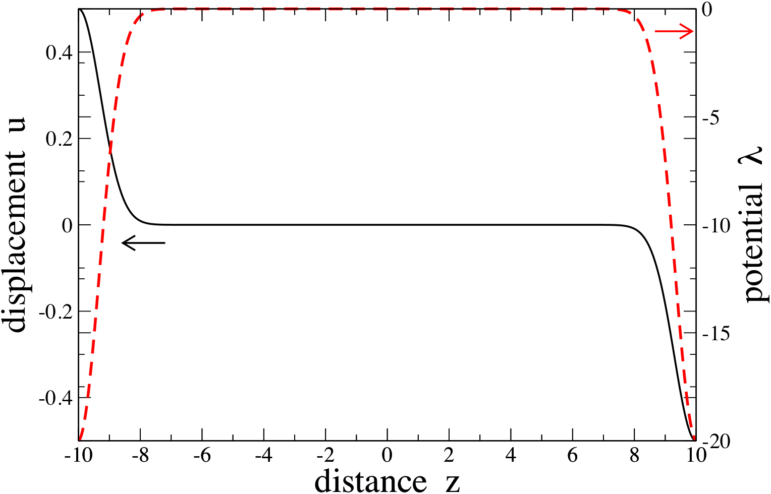
Figure 1: (Color online.) The displacement corresponding to a contraction near the edges. For clearly illustrating the contraction, we depict exaggerated displacements. In this sketch, the displacement (black solid) is given by Eq. (5) with $L=20,u_{0}=0.5,d=1$, and $k=1$ where the lattice constant set to unity. The effective potential (red dashed) is given by Eq. (6). The large (exaggerated) value of the displacement $u_{o}$ is chosen to vividly illustrate the contraction.

A displacement field describing a contraction along the $z$ direction is given by

$$u_{z}=\begin{cases}u_{0}[e^{-(z+L/2)^{2}/k^{2}}-e^{-(z-L/2)^{2}/k^{2}}]&\mbox{ for }|z|\leq L/2\\ 0&\mbox{ for }|z|>L/2\end{cases}.$$ (5)

The displacement thus occurs in some finite region (of scale $k$) about the edges. $u_{0}$ the maximum displacement, and with no displacement along the $x$ or $y$ directions, $u_{x}=u_{y}=0$.

The corresponding effective potential of Eq. (2) is given by

$$\lambda=\frac{2u_{0}d}{k^{2}}\Big{[}(z-\frac{L}{2})e^{-(dz-\frac{L}{2})^{2}/k^{2}}-(z+\frac{L}{2})e^{-(z+\frac{L}{2})^{2}/k^{2}}\Big{]}.$$ (6)

For $|z|>L/2$ (points outside the crystal), the supersolid order parameter $\psi=0$ and in Eq. (4) the effective potential $\lambda=\infty$. For small deformations, this attractive potential leads to the appearance of a weak bound state. For $z>0,~{}L/2\gg(L/2-z)\gg k\sqrt{\ln(2u_{0}d/k)}\equiv\epsilon/2$, the effective potential tends to zero, and the bound state wavefunction is of the form $\psi\sim\exp[\kappa(z-L/2)]$. A similar form is attained near the point $z=-L/2$. The value of $\kappa$ and thus of the bound state energy $E=-c\kappa^{2}$ can be computed in the standard way by integrating the Schrödinger equation once in a region of width $\epsilon$ across the point $z=L/2$ in an extension of the problem to $z>L/2$ in which the potential is symmetrized about the point $z=L/2$. As $|E|\ll|\lambda(z)|$ in the narrow region near the edges, Eq. (4) reads

$$-2\kappa=\left[\frac{d\psi}{dz}\right]^{L/2+\epsilon/2}_{L/2-\epsilon/2}=\frac{1}{c}\displaystyle\int_{L/2-\epsilon}^{L/2+\epsilon}\lambda(z)dz.$$ (7)

Ignoring exponentially small corrections, we attain that the bound state energy is

$$E=-\frac{d^{2}u_{0}^{2}}{4c}.$$ (8)

We will now employ the value of E to determine a change in the transition temperature. Within the GL theory, $a(T)\simeq\alpha(T-T_{c}^{0})$ near the transition temperature, where $T_{c}^{0}$ is the unaltered transition temperature and $\alpha>0$ is a constant. Writing $a+E=\alpha(T-T_{c}^{eff})$ where $T_{c}^{eff}$ is the effective transition temperature, we have

$$T_{c}^{eff}=T_{c}^{0}+\Delta T_{c},$$ (9)

with

$$\Delta T_{c}=\frac{d^{2}u^{2}_{0}}{4\alpha c}.$$ (10)

In other words, the region near the contracted edges has a higher transition temperature into the supersolid state than the bulk. Generally, the maximal displacement in Eqs. (5) and (13) can be of order $u_{0}\sim 0.1$ lattice constants as set by the Lindemann criterion of melting in most materials (or of $u_{0}\sim 0.2$ in solid ⁴He and potentially other quantum solids). lind In Eqs. (1) and (2), the parameters $c,d={\cal{O}}(1)$. We estimate a small enhancement of the transition temperature in the surface region. For parameters $\alpha=1/T_{c}^{0},d=1,u_{0}=0.1$, and $c=1$, we find from Eq. (10) a small enhancement compared to the bulk transition, $\Delta T_{c}=2.5\times 10^{-3}T_{c}^{0}$.

The effect of this shifted transition temperature is that, when a sample of contracted ⁴He is cooled down, the region near the edges would turn into supersolid at a higher temperature than the bulk of the crystal. Perusing the form of the supersolid order parameter $\psi$, and Eq. (7), we see that $\psi$ drops exponentially away with the boundary with a penetration depth $\ell=2c/(du_{0})$. With our previous estimates for parameters in Eq. (10) combined, we find that the penetration depth $\ell\sim 20$ lattice constants.

Returning to the NCRI KC ; London ; Fairbank ; Andron briefly discussed in the introduction, if the entire sample is rotating before the transition to a supersolid phase occurs, at some temperature higher than the normal transition to supersolid of bulk helium but low enough to make the edges become supersolid, the supersolid component in the edges will partially decouple from the bulk rotation. This situation is depicted schematically in Fig. (2).

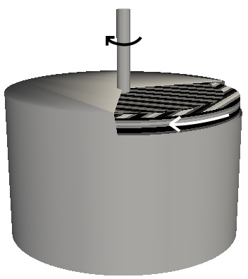
Figure 2: Under compression of the edges of the torsional oscillator, the rim attains a supersolid component at a higher temperature than the bulk does. On cooling down to this temperature, the supersolid fraction of the rim partially decouples from the bulk and outer chassis.

We now expand on the relation between the local value of the supersolid order parameter $\psi$ and the local effective transition temperature. Eq. (4) holds for all locations $-L/2\leq z\leq L/2$ (and trivially, of course, on any local segment within this region). We earlier solved Eq. (4) to find that the supersolid order parameter decays exponentially with a decay distance $\ell$ away from the boundary points $z=\pm L/2$. Thus, deep within the bulk, the supersolid order parameter was zero. We may examine Eq. (4) locally (with a local effective potential $\lambda(z)$) in order to see when we may attain a finite supersolid order parameter $\psi(z)$ at general locations $z$ away from the boundary.

As the displacement only occurs near the edges, and since the change in transition temperature is the result of the displacement, it is reasonable to assume that the change in transition temperature can only be detected in the region near the edges. For the region inside the crystal (far from the edge), the transition temperature should remain unaltered. Based on the observation, the transition temperature as a function of the z-axis (the axis parallel to the length of the crystal) could be described as

$$T_{c}^{eff}(z)=T_{c}^{0}+f(z)\left(\frac{d^{2}u^{2}_{o}}{4\alpha c}\right),$$ (11)

where $f(z)$ is a function that rapidly varies from $1$ at the boundaries $z=\pm L/2$ to zero for positions removed from the boundaries. An example is provided by

$$f(z)=e^{-(z-L/2)^{2}/k^{2}}+e^{-(z+L/2)^{2}/k^{2}}.$$ (12)

A contour plot of $T_{c}^{eff}$ is depicted in figure 3, for $L=20$ (we set the lattice constant to be unity), $k=1,T_{c}^{0}=2$ K, $u_{0}=0.5$ and $\frac{d^{2}u_{0}^{2}}{4\alpha c}=0.2$ K. The large (exaggerated) value of the displacement $u_{o}$ is chosen to lucidly illustrate a contraction as in, e.g., Fig. 1 and its effect.

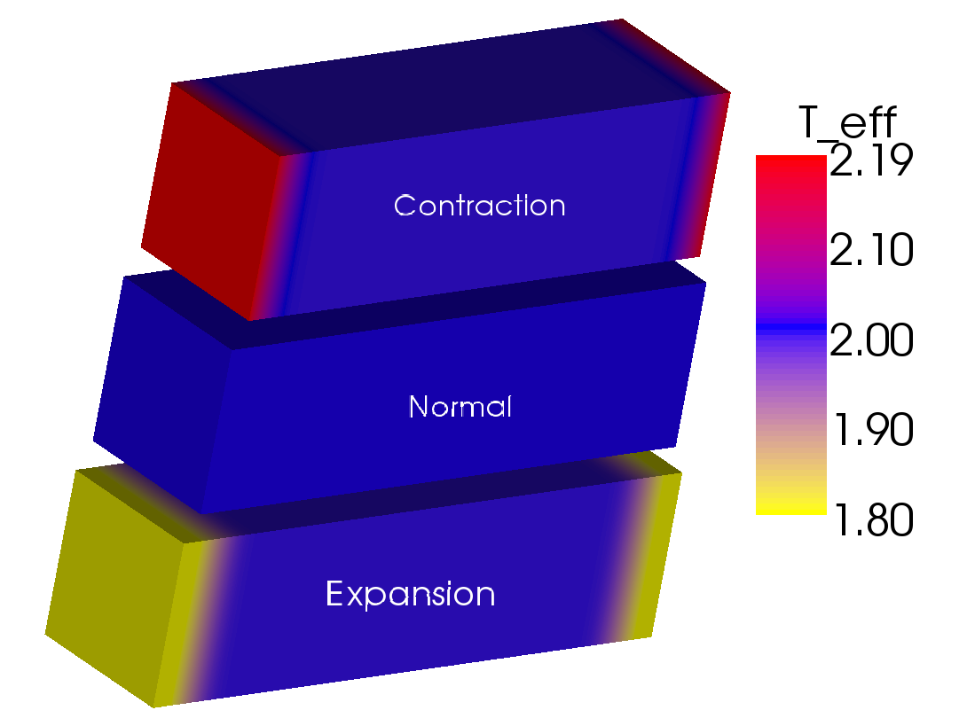
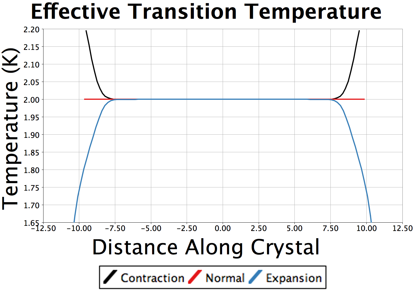
Figure 3: (Color online.) (a) The transition temperature along a slab is plotted in a contour map for different cases from top to bottom: a slab with contraction, a uniform slab, and a slab with expansion near its edges. Whenever the elastic deformations are present, the local supersolid transition temperature is altered by comparison to the uniform solid. Near the edges, where the elastic deformation is present, the supersolid transition temperature is altered: $T_{c}$ increases at the boundaries in the case of boundary contraction and decreases for an expansion near the boundaries. The dark (black) line is associated with contraction, red line with the normal crystal, and blue with the expansion. With the lattice constant to unity, the parameters $k=1,T_{c}^{0}=2$ K, $u_{0}=0.5$ and $\frac{d^{2}u_{0}^{2}}{4\alpha c}=0.2$ K. (b) We plot the effective transition temperature for an undeformed crystal (straight line), and that with a compression/expansion of its boundaries.

IV Expansion of edge boundaries

The situation of the expansion near the edge boundaries is schematically shown in Fig. 4. As in the case of contraction, this may be physically brought about by applying opposite stresses (e.g., shear stresses) on the two boundaries of the system. In an annular geometry similar to that in Fig.  2, an expansion may result by a difference in pressures between the inner and outer parts of the cylinder.

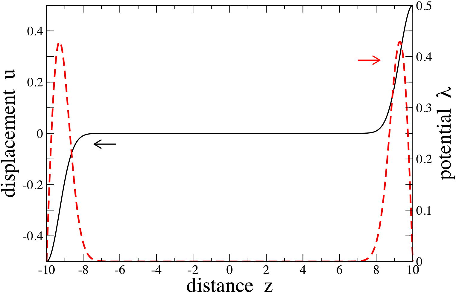
Figure 4: (Color online.) The displacement field corresponding to an expansion near the edges. Plotted is the displacement field (black solid) given by Eq. (13) with $L=20,u_{0}=0.5,d=1$ and $k=1$. The effective potential (red dashed) is given by Eq. (16). The large (exaggerated) displacement highlights the expansion near the boundaries.

A typical displacement field $\vec{u}$ is, in this case, given by

$$u_{z}=\begin{cases}u_{0}[e^{-(z-L/2)^{2}/k^{2}}-e^{-(z+L/2)^{2}/k^{2}}]&\mbox{for }|z|\leq L/2\\ 0&\mbox{for }|z|>L/2\end{cases},$$ (13)

and $u_{x}=u_{y}=0$. The variational equations give rise to a Schrödinger equation. The sign of $\lambda$ is flipped relative to the case of the contraction. In this case, $\lambda$ is everywhere positive reflecting a repulsive effective potential. This difference in sign gives rise to an important difference between expansion and contraction. In the case of expansion, the effective potential displays two peaks instead of two wells. In the absence of the two peaks, the problem reduces to that of a particle in an infinite potential well model. The wavefunction for the unperturbed ground state is now given by

$$\psi=\sqrt{\frac{2}{L}}\cos\left(\frac{\pi}{L}z\right).$$ (14)

The energy of such a bound state in a box of size $L$ is

$$E=\frac{\pi^{2}c}{L^{2}}.$$ (15)

Now, consider the perturbed state with the potential given by $\lambda=d\vec{\nabla}\cdot\vec{u}$ which reads

$$\lambda=\frac{2du_{0}}{k^{2}}\Big{[}(z+\frac{L}{2})e^{-(z+\frac{L}{2})^{2}/k^{2}}-(z-\frac{L}{2})e^{-(z-\frac{L}{2})^{2}/k^{2}}\Big{]}.$$ (16)

We may approximate $\lambda$ near its maxima by delta functions. The maxima occur at $z=\mp\frac{L}{2}\pm\frac{k}{\sqrt{2}}$. We express $\lambda$ as

$$\lambda=du_{0}\left[\delta[z-(\frac{L}{2}-\frac{k}{\sqrt{2}})]+\delta[z+(\frac{L}{2}-\frac{k}{\sqrt{2}})]\right].$$ (17)

The first order approximation to the perturbed ground state energy trivially yields

$$E^{\prime}=E+\displaystyle\int^{\infty}_{-\infty}\psi^{*}\lambda\psi dz=E+\frac{8du_{0}}{\pi}\sin\frac{k\pi}{L\sqrt{2}}.$$ (18)

Replicating the steps of Section III, we find that the effective transition temperature $T_{c}^{eff}$ for the case of expansion is

$$T_{c}^{eff}(z)=T_{c}^{0}-f(z)\left(\frac{\pi^{2}c}{\alpha L^{2}}+\frac{8du_{0}}{\alpha\pi}\sin\frac{k\pi}{L\sqrt{2}}\right).$$

In this case, as the system is cooled down, the faces would become supersolid after the bulk crystal as we cool down the crystal. A plot is given in Fig.  3 for $T_{c}^{0}=2$ K, $u_{0}=0.5,\frac{\pi^{2}c}{\alpha L^{2}}=0.02$ K, and $\frac{8du_{0}}{\alpha\pi}\sin\frac{k\pi}{L\sqrt{2}}=1$ K. As in our prior analysis of the contraction, the large value of $u_{0}$ in Fig. 4 is chosen to vividly illustrate the elastic distortion associated with an expansion.

It is worth highlighting the origin of the difference between the cases of edge contraction and expansion. Both cases have different divergences of the displacement field (and thus different local density profiles). The local mass or equivalently, the vacancy density is what couples to the supersolid order parameter. Note, in case of a superconductor it is the charge density that couples to the order parameter. Both the displacement field and the spatial gradient are odd under spatial reflection. In our case, $\vec{\nabla}\cdot\vec{u}$ is even under spatial reflection (it reflects the scalar mass density) and the two cases are physically very different even though the spatial profile of the displacement fields in both cases are related by a minus sign (see Eqs.(5) and (13)).

V Dislocations

Below, we will present detailed numerical and variational calculations of the local transition temperature due to an edge dislocation using the formalism that we have employed thus far in this work. For a discussion of dislocations in the quantum arena see, e.g., Ref. znmc, . An analysis analogous to ours was done by Toner Toner who reached similar conclusions as we have. Some time after we discussed this phenomenon us09 , Ref. filament, considered the problem of dislocation line filaments which become supersolid while the bulk is non-supersolid. This is markedly different from our approach where both the bulk and the dislocation core become supersolid at transition temperatures that differ by small amounts. The small change in the ordering temperature is imperative in our perturbative approach of linearly expanding $a(T)$ in Eq. (1) about the bulk supersolid transition temperature and in neglecting the cubic terms in Eq. (3) when solving the effective Schrödinger type equation of Eq. (4).

Many displacement fields can correspond to a given “Burgers vector” $\vec{b}$ describing a dislocation. The Burgers vector is defined by a circuit integral around a dislocation core kleinert $b_{\gamma}=(\oint_{K}d\vec{s}\cdot\vec{\nabla}u_{\gamma})$ for a large contour $K$ around the dislocation core) describing a dislocation. We will analyze one such particular set of displacement fields. All of these displacement fields are related to one another via a smooth deformation $\vec{u}\to\vec{u}+\vec{v}$. Here, $\vec{v}$ is a non-singular vector field with a vanishing associated circulation: $\oint_{C}d\vec{s}\cdot\vec{\nabla}v_{\gamma}=0$ around any closed contour $C$. As we saw in the earlier sections, a smooth displacement field (corresponding to, e.g., a contraction or an expansion) can, on its own, raise or lower the effective local supersolid transition temperature. Thus, the effective change in $T_{c}$, which we turn to next, will generally depend on the detailed form of the displacement fields $\vec{u}$ corresponding to a given dislocation. In what follows, we consider a particular minimal displacement field form that corresponds to symmetric unidirectional displacements about a lattice direction of an unstrained crystal. With $x$ and $y$ denoting the horizontal and vertical Cartesian directions, we consider a particular displacement field in Figs. 5(a)) and 5(b) that corresponds to a dislocation with a Burgers vector $\vec{b}=b\hat{e}_{x}$. In what follows, the spatial extent of the dislocation core will be set by $k$.

(a) An edge dislocation

(b) The displacement field corresponding to an edge dislocation

Figure 5: A schematic of an edge dislocation. At left (a), shown are rows of atoms. The presence of an edge dislocation is manifest in the appearance of a different number of vertical rows of atoms above and below the terminal dislocation point. The corresponding displacement field is shown at right (b).

The following displacement field describes such an edge dislocation,

$$\vec{u}(x,y)=-\frac{b}{2\pi}e^{-(x^{2}+y^{2})/k^{2}}sgn(x)\cos^{-1}\left(\frac{-y}{\sqrt{x^{2}+y^{2}}}\right)\hat{e}_{x},$$ (19)

where $sgn(x)$ is the sign of $x$, i.e., $sgn(x)=[2\theta(x)-1]$ with $\theta(x)$ the Heavyside function. In Eq. (19), the magnitude of the Burgers vector $b$ cannot exceed the inter-atomic lattice spacing. Furthermore, realistically, $k$ may be of order of 10 (lattice constants). We may derive an effective potential from the displacement in the same way we did for the above two cases (Eq. (2)). In this case, an analytical solution to Schrödinger equation is not possible and we will resort to a numerical solution. The effective potential energy is provided in Fig.  6.

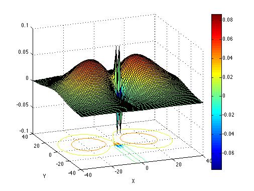
Figure 6: (Color online.) The effective potential energy of Eq. (V) corresponding to the displacement function of Eq. (19). In this figure, $b=d=c=$ and $k=10$. That is, $\beta=0.0135$ and $\sigma=0.0017$. The maximum strain is 0.086 (in units of the lattice constant).

We approximate the partial derivatives in the Schrödinger equation by finite differences and use the numerical Gauss-Seidel method for solving iteratively a system of linear equations in conjunction with over-relaxation. Our relaxation scheme shows that the wavefunction localizes rapidly to the region near the origin where the dislocation core sits. Both the initial seed and the final numerical result are depicted in Fig. 7.

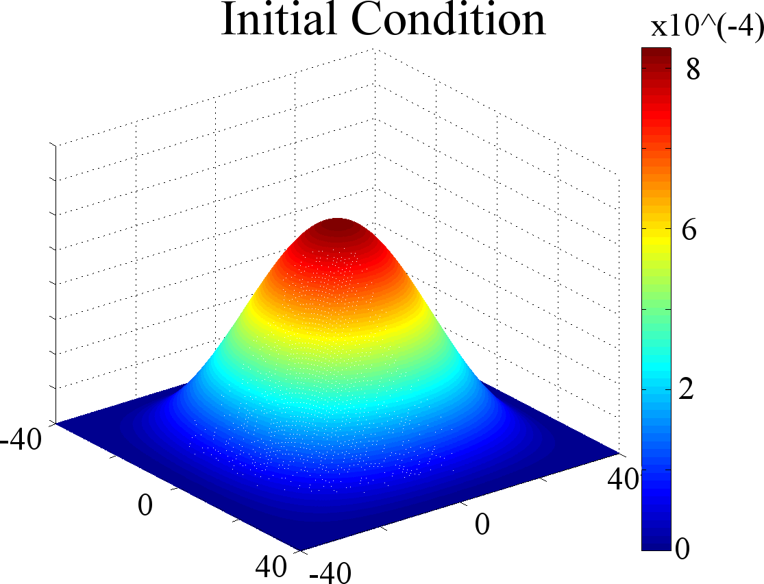
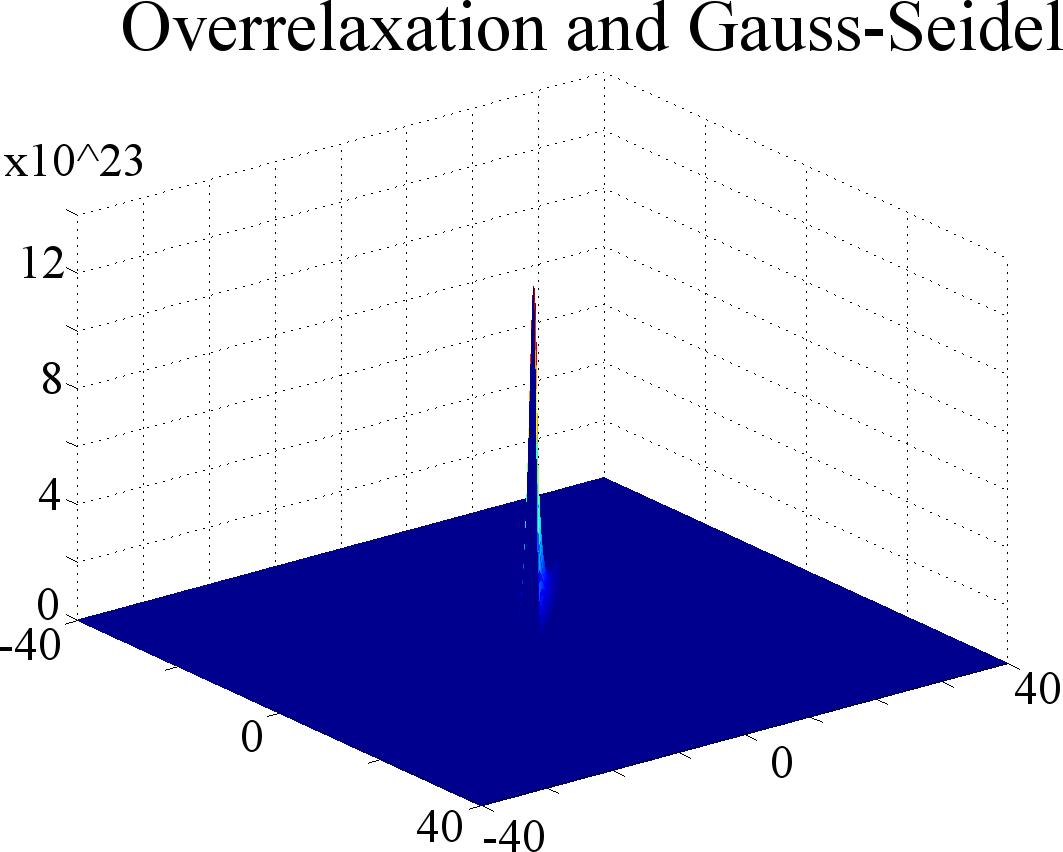
Figure 7: (Color online.) The supersolid order parameter associated with the effective potential of Fig. 6. Shown is the Gauss-Seidel solution of Eqs. (3) and (4) with $c=1$ for the dislocation profile of Eq. (19). Left: An initial seed state. Right: The final “wavefunction” (supersolid order parameter) $\psi$. The localized bound state of the order parameter is evident.

The numerical solution to the Schrödinger equation illustrates that there is a change in transition temperature.

We now turn to an approximate analytical solution. A contending variational state that is localized about the dislocation core is given by

$$\psi(x,y)=\sqrt{\frac{2\sigma}{\pi}}e^{-\sigma(x^{2}+y^{2})}.$$ (20)

From Eq. (19), we can compute the effective potential energy,

$$V \equiv\lambda=d(\vec{\nabla}\cdot\vec{u})$$

$$=\frac{bd}{2\pi}sgn(x)e^{-\sigma(x^{2}+y^{2})}\bigg{[}\frac{2x}{k^{2}}\cos^{-1}\left(\frac{-y}{\sqrt{x^{2}+y^{2}}}\right)$$

$$\qquad+\frac{y}{x(x^{2}+y^{2})}\bigg{]}.$$ (21)

The Hamiltonian $H=[-c\nabla^{2}+V]$ corresponds to the Schrödinger equation of Eq. (4). The expectation value is

$$\langle H\rangle=2c\sigma-\frac{\sigma bd}{2\sqrt{\pi k^{2}(2\sigma+\frac{1}{k^{2}})^{3}}}\geq E_{ground}.$$ (22)

An extremizing variational value of $\sigma$ is given by

$$\sigma=\frac{1}{2}\left(\left(\frac{3bd}{8\sqrt{\pi}ck^{4}}\right)^{2/5}-\frac{1}{k^{2}}\right).$$ (23)

Substituting the above equation into Eq. (22), we obtain

$$\langle H\rangle=c(\beta-\frac{1}{k^{2}})-bd\left(\frac{\beta k^{2}-1}{4\sqrt{\pi}\beta^{3}k^{4}}\right),$$ (24)

where $\beta=\left(\frac{3bd}{8\sqrt{\pi}ck^{4}}\right)^{2/5}$. Similar to the earlier two cases of boundary deformations, the effective transition temperature can be found by approximating $a(T)\approx\alpha\,(T-T_{c}^{0})$. The transition temperature

$$T_{c}^{eff}=T_{c}^{0}-\frac{1}{\alpha}c\left(\left(\beta-\frac{1}{k^{2}}\right)+bd\left(\frac{\beta k^{2}-1}{4\sqrt{\pi}\beta^{3}k^{4}}\right)\right).$$ (25)

In Fig. 8, we plot $\Delta T_{c}=T_{c}^{eff}-T_{c}^{0}$ for different Burgers vectors $b$ as a function of dislocation core size $k$ for fixed values of the parameters in the GL functional of Eqs. (1) and (2): $c=d=1$. Depending on the choice of parameters an increase or decrease in the local transition temperature relative to a bulk transition is possible. Assuming a typical Burgers vector magnitude of $b=1$ for an edge dislocation in an hcp crystal, with parameters $c=d=1$, a core size radius of $R=k/\sqrt{2}<3.5$ lattice constants will result in a supersolid dislocation core prior to the bulk supersolid transition.

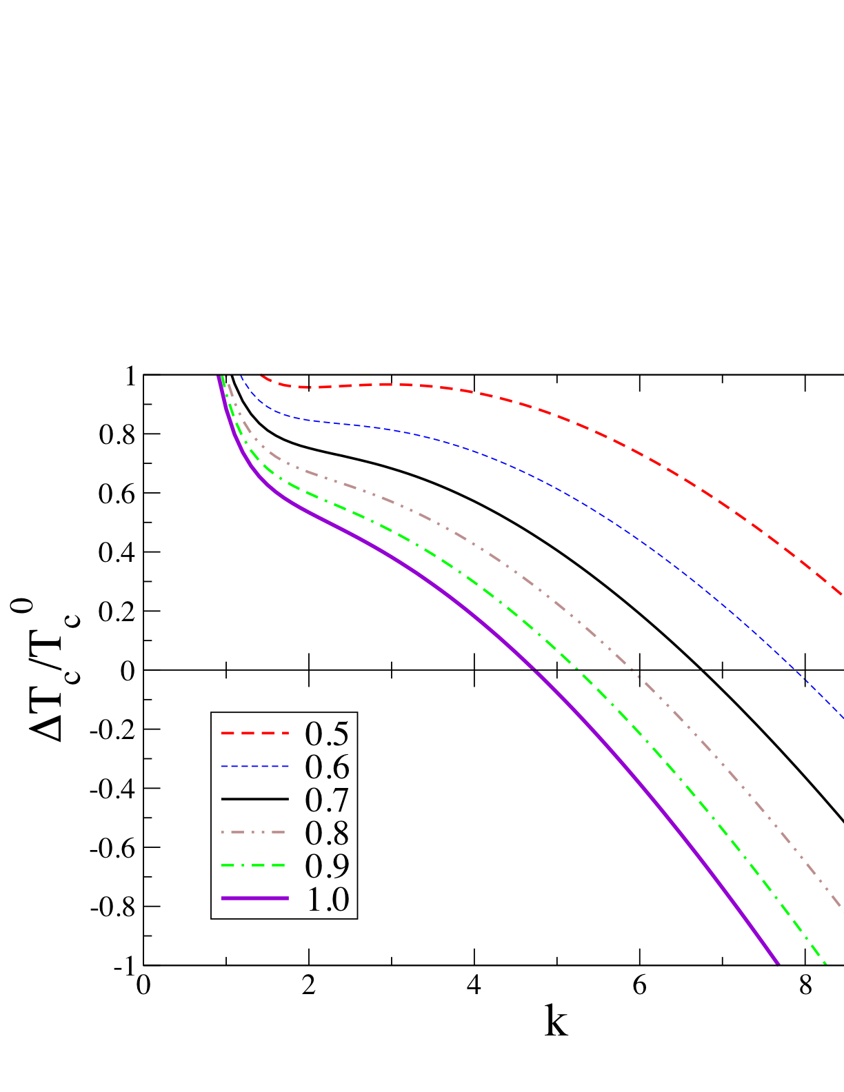
Figure 8: (Color online.) The shift in the local transition temperature in the vicinity of the dislocation core for different values of Burgers vector $b=0.5,\dots,1.0$ as a function of core size $k$. The other parameters are set as $c=d=1$ and $\alpha=1/T_{c}^{0}$.

VI Conclusions

In summary, we find that elastic deformations in supersolid lead to local changes in the transition temperature. For a positive coupling constant $d$ in Eq. (2) we obtain the results:

1. Edge contraction increases the supersolid transition temperature at and near the edges.

2. Edge expansion decreases the supersolid transition temperature at and near the edges.

3. The local supersolid transition may be enhanced or suppressed near a dislocation core.

This implies the observation of interesting effects. For example, for edge contractions, we would find that, below a certain temperature that is higher than the supersolid transition temperature, a sample of supersolid would have its supersolid edges partially decouple from its bulk crystal. Of course, the effects of elastic deformations on the supersolid transition are not limited to the few selected cases studied here. For example, the same physics applies to point defects like interstitials and vacancies, as well as to extended defects like grain boundaries and inclusions or voids. The above conclusions were based on the assumption of a positive coupling constant $d$ in Eq. (2). Formally, for negative $d$, our conclusions would have been inverted- an expansion would enhance the local supersolid transition while a contraction would reduce the supersolid transition temperature.

Similar effects are found elsewhere in regions that locally expand or contract. In Ref. znmc, it was shown how a dislocation condensate may generally enhance and trigger superfluid behavior via a Higgs type mechanism. The presented GL approach of elastic deformations on the supersolid transition temperature is quite general and also applies to superconductors. In fact, dislocation defects and lattice-mismatched interfaces in superconductors are known to create nonuniform strain and changes to the superconducting transition temperature, which have been studied extensively.Fogel2002 Thus, our calculations of the changes in the local transition temperature due to a nonuniform elastic strain coupling in a Ginzburg-Landau approach are not limited to supersolidity and may as well apply to superconductivity.

VII Acknowledgments

This work was partially supported by the Center for Materials Innovation (CMI) of Washington University, St. Louis and by the US Dept. of Energy at Los Alamos National Laboratory under contract No. DEAC52-06NA25396. We are grateful to A. T. Dorsey, J. Beamish, J. C. Davis, and J.-J. Su for many stimulating discussions.

References

- (1) O. Penrose and L. Onsager, Phys. Rev. 104, 576 (1956); G. V. Chester and L. Reatto, Phys. Rev. 155, 88 (1967); A. F. Andreev and I. M. Lifshitz, Sov. Phys. JETP 29, 1107 (1969); L. Reatto, Phys. Rev. 183, 334 (1969); A. J. Leggett, Phys. Rev. Lett. 25, 2543 (1970); P.W. Anderson, Basic Notions of Condensed Matter Physics, (Benjamin, Menlo Park, CA), Ch. 4, 143 (1984); G. G. Batrouni, R. T. Scalettar, G. T. Zimanyi, and A. P. Kampf, Phys. Rev. Lett. 74, 2527 (1995); G. G. Batrouni and R. T. Scalettar, Computer Physics Communications 97, 63 (1996); D. M. Ceperley and B. Bernu, Phys. Rev. Lett. 93, 155303 (2004); W. Saslow, Phys. Rev. B 71, 092502 (2005); T. Suzuki and N. Kawashima, Phys. Rev. B 75, 180502 (R) (2007); A. Stoffel and M. Gulacsi, Europhysics Letters 85, 20009 (2009).
- (2) G.V. Chester, Phys. Rev. A 2, 256 (1970).
- (3) N. Prokof’ev, Adv. in Phys. 56 2, 381 (2007).
- (4) E. Kim and M. H. W. Chan, Nature (London) 427, 225 (2004); Science 305, 1941 (2005); Phys. Rev. Lett. 97, 115302 (2006); A. S. C. Rittner and J. D. Reppy, Phys. Rev. Lett. 97, 165301 (2006); ibid. 98, 175302 (2007); Y. Aoki, J. C. Graves, and H. Kojima, Phys. Rev. Lett. 99, 015301 (2007); J. Low Temp. Phys. 150, 252 (2008); M. Kondo, S. Takada, Y. Shibayama, and K. Shirahama, J. Low Temp. Phys. 148, 695 (2007); A. Penzev, Y. Yasuta, and M. Kubota, J. Low Temp. Phys. 148, 677 (2007); Phys. Rev. Lett. 101, 065301 (2008); D. Y. Kim, S. Kwon, H. Choi, H. C. Kim, E. Kim, New J. Phys. 12, 033004 (2010); H. Choi, S. Kwon, D.Y. Kim, E. Kim, Nature Physics 6, 424 (2010); Yu. Mukharsky, A. Penzev, and E. Varoquaux, Phys. Rev. B 80, 140504(R) (2009)
- (5) E. Pratt, B. Hunt, V. Gadagkar, M. Yamashita, M. J. Graf, A. V. Balatsky, and J. C. Davis, Science 332, 821 (2011).
- (6) F. London, Superfluids (Wiley, New York (1954)), vol. II, p. 144.
- (7) G. B. Hess and W. M. Fairbank, Phys. Rev. Lett. 19, 216 (1967).
- (8) E. I. Andronikashvili, J. Phys. (USSR) 10, 201 (1946); E. I. Andronikashvili and Yu. G. Mamaladze, Rev. Mod. Phys. 38, 567 (1966).
- (9) S. Sasaki, R. Ishiguro, F. Caupin, H. J. Maris, and S. Balibar, Science 313, 1098 (2006).
- (10) A. V. Balatsky, M. J. Graf, Z. Nussinov, and S. A. Trugman, Phys. Rev. B 75, 094201 (2007); J.-J. Su, M. J. Graf, and A. V. Balatsky, J. Low Temp. Phys. 159, 431 (2010).
- (11) A. S. C. Rittner and J. D. Reppy, Phys. Rev. Lett. 98, 175302 (2007).
- (12) Y. Aoki, M. C. Keiderling, and H. Kojima, Phys. Rev. Lett. 100, 215303 (2008).
- (13) Z. Nussinov, A. V. Balatsky, M. J. Graf, and S. A. Trugman, Phys. Rev. B 76, 014530 (2007); M. J. Graf, Z. Nussinov, and A. V. Balatsky, J. Low Temp. Phys. 158, 550 (2010); J.-J. Su, M. J. Graf, and A. V. Balatsky, Phys. Rev. Lett. 105, 045302 (2010); M. J. Graf, A. V. Balatsky, Z. Nussinov, I. Grigorenko, and S.A. Trugman, J. Phys.: Conf. Ser. 150, 032025 (2009);
- (14) C-D. Yoo and A. Dorsey, Phys. Rev. B 79, 100504 (2009).
- (15) D. A. Huse and Z. U. Khandker, Phys. Rev. B 75, 212504 (2007).
- (16) J. Day, O. Syshchenko, and J. Beamish, Phys. Rev. B 79, 214524 (2009); O. Syshchenko, J. Day, and J. Beamish, Phys. Rev. Lett. 104, 195301 (2010).
- (17) I. Iwasa, Phys. Rev. B 81, 104527 (2010).
- (18) A. F. Andreev, JETP Lett. 85, 585 (2007); A. F. Andreev, JETP 109, 103 (2009).
- (19) S. E. Korshunov, JETP Lett. 90, 156 (2009).
- (20) X. Rojas, A. Haziot, V. Bapst, S. Balibar, and H. J. Maris, Phys. Rev. Lett. 105, 145302 (2010)
- (21) L. C. Struick, Physical Aging in Amorphous Polymers and Other Materials (Elsevier, Amsterdam,1978). A. P. Young (Editor), Spin Glasses and Random Fields, Series on Directions in Condensed Matter Physics, Vol. 12 (World Scientific, Singapore, 1998).
- (22) G. Biroli, B. Clark, L. Foini, and F. Zamponi, Phys. Rev. B 83, 094530 (2011)
- (23) M. Boninsegni, N. Prokof ev, and B. Svistunov, Phys. Rev. Lett. 96, 105301 (2006); J. Wu and P. Phillips, Phys. Rev. B 78, 014515 (2008); G. Biroli, C. Chamon, and F. Zamponi, Phys. Rev. B 78, 224306 (2008); Z. Nussinov, Physics 1, 40 (2008).
- (24) J. Zannen, Z. Nussinov, and S. I. Mukhin, Ann. Phys. 310, 181 (2004); V. Cvetkovic and J. Zaanen, Phys. Rev. Lett. 97, 045701 (2006); V. Cvetkovic, Z. Nussinov, S. Mukhin, and J. Zaanen, Europhys. Lett. 81, 27001 (2008).
- (25) A. V. Balatsky and E. Abrahams, J. of Superconductivity and Novel Magnetism 19, 395 (2006).
- (26) A. T. Dorsey, P. M. Goldbart, and J. Toner, Phys. Rev. Lett. 96, 055301 (2006).
- (27) J. Toner, Phys. Rev. Lett. 100, 035302 (2008).
- (28) H. P. Büchler and G. Blatter, Phys. Rev. Lett. 91, 130404 (2003); V. W. Scarola and S. Das Sarma, Phys. Rev. Lett. 95, 033003 (2005); A. Koga, T. Higashiyama, K. Inaba, S. Suga, and N. Kawakami, J. Phys. Soc. Japan 77, 073602 (2008); T. Keilmann, I. Cirac, and T. Roscilde, Phys. Rev. Lett. 102, 255304 (2009).
- (29) P. Sengupta and C. D. Batista, Phys. Rev. Lett. 98, 227201 (2007).
- (30) For a review, see Lattice Effects in High-Tc Superconductors, eds. Y. Bar-yam, T. Egami, J. Mustre-de Leon, and A. R. Bishop (World Scientific, Singapore, 1992); Nanoscale Phase Separation and Colossal Magnetoresistence, ed. E. Dagotto (Springer, New York, 2003); Instrinsic Multiscale Structure and Dynamics in Complex Electronic Oxides, eds. A. R. Bishop, S. R. Shenoy, and S. Sridhar (World Scientific, Singapore, 2003).
- (31) Jian-Xin Zhu, K. H. Ahn, Z. Nussinov, T. Lookman, A. V. Balatsky, and A. R. Bishop, Phys. Rev. Lett. 91, 057004 (2003).
- (32) A. V. Gurevich and E. A. Pashitskii, Low Temp. Phys. 24, 794 (1998).
- (33) G. J. Sizoo and H. K. Onnes, Commun. Phys. Lab. Univ. Leiden, No. 180b (1925).
- (34) D. H. Bowen, in R.S. Bradley(ed.), High Pressure Physics and Chemistry I, Academic Press, New York, 353 (1963); J. S. Schilling, Proceedings of the NATO Advanced Research Workshop Frontiers of High Pressure Research II: Application of High Pressure to Low-Dimensional Novel Electronic Materials, 345 edited by H. D. Hochheimer, B. Kuchta, P. K. Dorhout, and J.L. Yarger (Kluwer Academic Pub., Boston,2001).
- (35) M. Ozaki et al., Prog. Theor. Phys. 75, 442 (1986)
- (36) J.J. Betouras, V.A. Ivanov, and F.M. Peeters, Eur. Phys. J. B 31, 349 (2003)
- (37) L. D. Landau and E. M. Lifshitz, Statistical Physics Part 2, Butterworth-Heinemann, Boston (1999).
- (38) M. Tinkham, Introduction to Superconductivity, 2nd edition, McGraw-Hill, New York (1996).
- (39) J. Friedel, Dislocations, Pergamon press, New York, 1954; F. R. N. Nabarro, Theory of Dislocations, Clarendon, Oxford, 1967; J. P. Hirth and J. Lothe, Theory of Dislocations, McGraw- Hill, New York, 1968; H. Kleinert, Gauge fields in Condensed Matter, Vol. II: Stresses and Defects, Differential Geometry, Crystal Defects (World Scientific, Singapore, 1989).
- (40) J. A. Aronovitz, P. Goldbart, and G. Mouzurkewich, Phys. Rev. Lett. 64, 2799 (1990).
- (41) J-J. Su, M. J. Graf, and A. V. Balatsky. arXiv:1105.5343 (2011)
-
(42)
Eq. (3) could also be solved in the presence of the cubic term,
albeit not giving any new insight relative
to our linearized differential equation of Eq. (4).
Throughout this work, we will assume a system that is symmetric about the origin, with a unidirectional axis of length along
which the displacements occur ().
For real , with boundary condition ,
multiplying Eq. (3) by and integrating,
we arrive at the general implicit relation
for . Eq. (26) may be inverted to determine for negative . For , in a system with displacements that are symmetric about , .(26) - (43) D. Lim, V. K. Thormoelle, R. D. Averitt, Q. X. Jia, K. H. Ahn, M. J. Graf, S. A. Trugman, and A. J. Taylor, Phys. Rev. B 71, 134403 (2005).
- (44) H. R. Glyde, Excitations in Liquid and Solid Helium (Oxford: Clarendon, 1994) C. Cazorla and J. Boronat, J. Phys.: Condens. Matter 20, 015223 (2008); D. A. Arms, R. S. Shah, and R. O. Simmons, Phys. Rev. B 67, 094303 (2003).
- (45) T. Arpornthip, A. V. Balatsky, M. J. Graf, and Z. Nussinov, arXiv: 0912.4787 (2009).
- (46) D. Goswami, K. Dasbiwas, C.-D. Yoo, and A. T. Dorsey, arXiv:1103.0057 (2011).
- (47) N. Ya. Fogel, E. I. Buchstab, Yu. V. Bomze, O. I. Yuzephovich, A. Yu. Sipatov, E. A. Pashitskii, A. Danilov, V. Langer, R. I. Shekhter, and M. Jonson, Phys. Rev. B 66, 174513 (2002); P. P. Pal-Val, V. D. Natsik, and L. N. Pal-Val, Low Temp. Phys. 32, 169 (2006); G. J. van Gurp and D. J. van Ooijen, J. de Physique, Colloque C 3, Suppl. 7-8, 51 (1966).