UMISS-HEP-2009-02

Department of Physics and Astronomy,
             University of Mississippi,
            Lewis Hall, University, MS, 38677.

1 Introduction

The flavor sector of the Standard Model(SM) is poorly understood. The origin of masses and mixing and CP violation in the quark and lepton sector is unknown. Another mystery is the rare Flavor Changing Neutral Current processes. Flavor Changing Neutral Current (FCNC) processes in the Standard Model(SM) do not arise at tree level, and are highly suppressed. Many extensions of the SM naturally have FCNC processes that occur at tree or loop level. Hence, measurements of FCNC processes can put strong constraints on new physics (NP) that may be discovered at present colliders like the Tevatron or the LHC. In that sense, flavor data can complement the new physics search at colliders.

Effects from new physics can cause deviations from the SM predictions. These deviations are expected to be more pronounced in rare FCNC processes as they are suppressed in the SM. The B factories have made several measurements of FCNC processes in the bottom sector and have put strong constraints on new physics. Here we will be concerned with constraints on the $b\to s\gamma$ and $b\to sZ$ transitions. New physics in the former are constrained by better measurements of the $b\to s\gamma$ rate [2] and a better understanding of the SM [3] contribution to the process. The later transition is constrained by $B_{s}$ mixing, $b\to sll$ and also possible hints of new physics in decays like $B\to K\pi,\phi K_{s}$ etc [4, 5].

There are no measurements of FCNC in the top sector. There are 95% C.L bounds, $t\to q(=u,c)\gamma<5.9\times 10^{-3}$ and $t\to q(=u,c)Z<0.037$ [6]. In the SM the branching ratios for the rare FCNC decays $t\to cV$ where $V=g,\gamma,Z$ are tiny [7, 8]. The small mass of the internal quarks in the SM loop diagram makes FCNC effects in the top sector much smaller than FCNC effects in the bottom sector. Hence, FCNC processes in the top sector are excellent probes of new physics.

The LHC will be a top factory allowing the possible detection of FCNC effects in the top sector [9]. One can hope to measure $t\to q(=u,c)Z$ with branching ratios in the range $6.1\times 10^{-5}-3.1\times 10^{-4}$ while $t\to q(=u,c)\gamma$ can be measured with branching ratios in the range $1.2\times 10^{-5}-4.1\times 10^{-5}$. New physics searches via the top quark decays have been extensively analyzed in the literature in specific models [10]. In this paper we focus on a model independent study of the non-SM FCNC effects in the top sector. In this framework, imposing the constraints on $b\to sV,V=\gamma,Z$ transitions as well as constraints from top branching ratios measurements, we predict the size of rare FCNC $t\to cV,V=\gamma,Z$ decays.

In our approach, we write down higher dimension operators which are invariant under the SM gauge group that generate the anomalous $t\to cV,V=\gamma,Z$ couplings. As the left-handed top and the left-handed bottom are in the same $SU(2)_{L}$ doublet the $tcV$ and the $bsV$ couplings are related. We consider two operators that can generate the $tcV$ and $bsV$ couplings. One involves the $SU(2)_{L}$ gauge fields and the other the $U(1)_{Y}$ gauge field. We choose the size of the couplings to be the same size as the $SU(2)_{L}$ gauge coupling, $g$, and the $U(1)_{Y}$ gauge coupling $g^{\prime}$. This choice for the size of the anomalous coupling is motivated by the assumption that the physics that generates the anomalous couplings are weakly coupled. Constraints from $b\to s\gamma$ force the couplings between the two operators to follow the same relation as the one between the $U(1)_{Y}$ and $SU(2)_{L}$ gauge couplings in the SM to a very good approximation. Assuming such a relation between the two couplings, the $b\to s\gamma$ constraint is eliminated and all predictions are found to depend on a single coupling associated with the $SU(2)_{L}$ gauge field. With the size of this coupling of the same order as $g$, all low energy constraints are found to be satisfied. The operators also generate a $t\to sW$ vertex and for the anomalous coupling $\sim g$, the corrections to the branching ratio for $t\to sW$ from new physics is found to be consistent with the top branching fraction measurements. Finally, predictions are made for $t\to c\gamma,t\to cZ$ and $t\to sW$ transitions.

There have been previous attempts [11, 12, 13] to make predictions for rare top processes using constraints from $B$ decays, specifically $b\to s\gamma$, in an effective Lagrangian approach. There are several differences between this work and the previous work. First, in the previous work the $tc\gamma$ and $tcZ$ couplings are independent while in our work they are related as our anomalous couplings are generated by operators invariant under the SM gauge group. Second, in the previous work constraints on the anomalous $tcZ$ and $tc\gamma$ couplings are obtained from FCNC effects in the down sector generated though loop effects. In our work, for the considered size of the couplings, we find that loop effects are sufficiently small to be consistent with experiments and therefore do not introduce any additional constraints. The size of the anomalous couplings are fixed from tree processes and hence these couplings are quite strongly constrained. As indicated above, we also take into account experimental constraints on top branching fractions.

Finally, a unique feature of the operators in the effective Lagrangian in our approach is that they are momentum dependent and therefore contributions to FCNC effects in the top sector are enhanced typically by a factor $\sim{m_{t}^{2}\over m_{b}^{2}}$ relative to the ones in the bottom sector. Note that, it has been speculated in the past that FCNC effects in the top sector may be enhanced because of its heavy mass. This has motivated specific ansatz for the FCNC vertices with enhanced effect in the top sector[14].

In our approach, the anomalous couplings in the bottom and top sector are related. This is true only for certain classes of models. However, the connection between the top and bottom sectors is not generic as far as FCNC effects are concerned. In the two higgs doublet model, for instance, FCNC arise in the bottom and the top sector at the tree or loop level. However, any connection between the effects in the two sectors are strongly dependent on the structure of the Yukawa couplings in the up and the down quark sectors. Within specific models of the Yukawa structures one can relate FCNC effects in the top and the bottom sector in new physics models [15, 16, 17].

The paper is organized in the following manner. In sec. 1 we write down the effective Hamiltonian that generates the $t\to cV(=\gamma,Z)$ transitions. The vertices for $b\to sV,t\to cV$ as well as $b\to cW$ and $t\to sW$ are written down. Constraints on these couplings are obtained. In the next section, sec. 2, we make predictions for the processes $t\to cV$, $V=\gamma,Z$, and $t\to sW$. In the final section, we present our conclusions.

2 Effective Lagrangian

In this section we write the effective Lagrangian that generates to $t\to cV,V=\gamma,Z$ transitions. We write the effective Hamiltonian as,

$${\cal L} = {\cal L}_{SM}+\sum_{i}\frac{c_{i}{\cal O}_{i}}{\Lambda^{2}},\$$ (1)

where ${\cal O}_{i}$ are dimension 6 operators.

We will concentrate on the following two operators [18],

$${\cal O}_{W} = i\bar{Q}_{i}\tau^{a}\gamma^{\mu}D_{\nu}Q_{j}W^{a\mu\nu},$$

$${\cal O}_{B} = i\bar{Q}_{i}\gamma^{\mu}D_{\nu}Q_{j}B^{\mu\nu},\$$ (2)

where $Q_{i,j}$ are the left-handed quark doublets, $i,j$ are the generation indices that refer to the second and third families respectively, and

$${\vec{D}_{\mu}}={\vec{\partial}}_{\mu}+igA_{\mu}^{a}\frac{\tau^{a}}{2}+ig^{\prime}B_{\mu}\frac{Y}{2}.$$

Hence we rewrite Eq. 1 as,

$${\cal L} = {\cal L}_{SM}+\frac{a_{W}{\cal O}_{W}+a_{B}{\cal O}_{B}}{\Lambda^{2}},\$$ (3)

As indicated in the previous section, the operators generate FCNC vertices with a $q^{2}$ dependence resulting in new physics FCNC effects in the top sector that are enhanced by a factor of $(m_{t}/m_{b})^{2}$ compared to new physics effects in the bottom sector. Such $q^{2}$ dependent operators were previously considered in the context of single top production[19]. One can also write down operators involving the Higgs field which can generate top FCNC processes[20]. Since, the mechanism of electroweak symmetry breaking and the Higgs sector of the SM are untested we will not consider those operators in our analysis. Now, before we go into the details of the calculations, it is worthwhile to see how such interactions might arise. Consider the interaction involving only the second and third family quarks of the type:

$${\cal L}_{0} = C_{3}\bar{Q}_{3}{\widetilde{Q}}_{3}{\widetilde{X}}+C_{2}\bar{Q}_{2}{\widetilde{Q}}_{2}{\widetilde{X}}+h.c,\$$ (4)

where we have suppressed any particle indices. The ${\widetilde{X}}$ could be a scalar/pseudoscalar, vector/axial vector etc. and the ${\widetilde{Q}}_{3}$ could be spin 0 or spin ${1\over 2}$ objects. Let us now suppose there is mixing such that in the mass basis,

$$\widetilde{Q}_{2}\rightarrow\widetilde{Q}_{2}\cos{\phi}-\widetilde{Q}_{3}\sin{\phi},$$

$$\widetilde{Q}_{3}\rightarrow\widetilde{Q}_{2}\sin{\phi}+\widetilde{Q}_{3}\cos{\phi},\$$ (5)

where $\phi$ is the mixing angle. One can then rewrite, Eq. 4 as,

$${\cal L}_{0} = C_{3}\bar{Q}_{3}{\widetilde{Q}}_{3}{\widetilde{X}}\cos{\phi}+C_{3}\bar{Q}_{3}{\widetilde{Q}}_{2}{\widetilde{X}}\sin{\phi}+C_{2}\bar{Q}_{2}{\widetilde{Q}}_{2}{\widetilde{X}}\cos{\phi}-C_{2}\bar{Q}_{2}{\widetilde{Q}}_{3}{\widetilde{X}}\sin{\phi}$$ (6)

$$+h.c\$$

Now we consider vertex corrections involving an intermediate $\widetilde{Q}_{3}$ or $\widetilde{Q}_{2}$ and $\widetilde{X}$. These corrections will generate the following vertices:

$$\bar{Q}_{2}Q_{3}V\equiv C_{2}C_{3}^{*}\left[f(\widetilde{Q}_{2})-f(\widetilde{Q}_{3})\right]\sin{\phi}\cos{\phi}$$

$$\bar{Q}_{3}Q_{3}V\equiv|C_{3}|^{2}\left[f(\widetilde{Q}_{3})\cos^{2}{\phi}-f(\widetilde{Q}_{2})\sin^{2}{\phi}\right]$$

$$\bar{Q}_{2}Q_{2}V\equiv|C_{2}|^{2}\left[f(\widetilde{Q}_{2})\cos^{2}{\phi}-f(\widetilde{Q}_{3})\sin^{2}{\phi}\right],\$$ (7)

where $V$ is the $W,Z,\gamma$ and $f^{\prime}s$ are the loop functions. It is clear that by proper choice of the parameters one can make the second operator, $\bar{Q}_{3}Q_{3}V$, small enough without suppressing the first flavor changing operator. The second operator can contribute to $Z\to\bar{b}_{L}b_{L}$ where new physics effects are strongly constrained [6]. This is just a scenario where the structure in Eq. 2 may be generated. Since we are adopting a model independent approach, we will not discuss specific models anymore.

These operators in Eq. 2 lead to the following interactions,

$${\cal L}_{C} = i\frac{a_{W}}{\sqrt{2}\Lambda^{2}}\left[\bar{c}\gamma_{\mu}(1-\gamma_{5})\partial_{\nu}bW^{+\mu\nu}+\bar{s}\gamma_{\mu}(1-\gamma_{5})\partial_{\nu}tW^{-\mu\nu}\right],$$

$${\cal L}_{tcZ} = i\frac{a_{W}c-a_{B}s}{{2\Lambda^{2}}}\left[\bar{c}\gamma_{\mu}(1-\gamma_{5})\partial_{\nu}tZ^{\mu\nu}\right],$$

$${\cal L}_{tc\gamma} = i\frac{a_{W}s+a_{B}c}{{2\Lambda^{2}}}\left[\bar{c}\gamma_{\mu}(1-\gamma_{5})\partial_{\nu}tA^{\mu\nu}\right],$$

$${\cal L}_{bsZ} = i\frac{-a_{W}c-a_{B}s}{{2\Lambda^{2}}}\left[\bar{s}\gamma_{\mu}(1-\gamma_{5})\partial_{\nu}bZ^{\mu\nu}\right],$$

$${\cal L}_{bs\gamma} = i\frac{-a_{W}s+a_{B}c}{{2\Lambda^{2}}}\left[\bar{s}\gamma_{\mu}(1-\gamma_{5})\partial_{\nu}bA^{\mu\nu}\right],\$$ (8)

where $c=\cos{\theta_{W}}$ and $s=\sin{\theta_{W}}$, with $\theta_{W}$ being the Weinberg angle.

The Lagrangian above generates momentum dependent vertices. We can combine the processes as $t(p)\to c(k)V(q)$ and $b(p)\to s(k)V(q)$, where $V=W,Z,\gamma$. For $b$ decays the massive vector bosons have to be off-shell. The vertices for various processes can now be written as,

$${\cal L}_{bcW} = -i\frac{a_{W}}{\sqrt{2}\Lambda^{2}}\left[\bar{c}\gamma_{\mu}(1-\gamma_{5})\left(q^{\mu}p^{\nu}-q\cdot p\delta^{\mu\nu}\right)bW^{+\nu}\right],$$

$${\cal L}_{tsW} = -i\frac{a_{W}}{\sqrt{2}\Lambda^{2}}\left[\bar{s}\gamma_{\mu}(1-\gamma_{5})\left(q^{\mu}p^{\nu}-q\cdot p\delta^{\mu\nu}\right)bW^{-\nu}\right],$$

$${\cal L}_{tcZ} = -i\frac{a_{W}c-a_{B}s}{2\Lambda^{2}}\left[\bar{c}\gamma_{\mu}(1-\gamma_{5})\left(q^{\mu}p^{\nu}-q\cdot p\delta^{\mu\nu}\right)tZ^{\nu}\right],$$

$${\cal L}_{tc\gamma} = -i\frac{a_{W}s+a_{B}c}{{2\Lambda^{2}}}\left[\bar{c}\gamma_{\mu}(1-\gamma_{5})\left(q^{\mu}p^{\nu}-q\cdot p\delta^{\mu\nu}\right)tA^{\nu}\right],$$

$${\cal L}_{bsZ} = -i\frac{-a_{W}c-a_{B}s}{{2\Lambda^{2}}}\left[\bar{s}\gamma_{\mu}(1-\gamma_{5})\left(q^{\mu}p^{\nu}-q\cdot p\delta^{\mu\nu}\right)bZ^{\nu}\right],$$

$${\cal L}_{bs\gamma} = -i\frac{-a_{W}s+a_{B}c}{{2\Lambda^{2}}}\left[\bar{s}\gamma_{\mu}(1-\gamma_{5})\left(q^{\mu}p^{\nu}-q\cdot p\delta^{\mu\nu}\right)bA^{\nu}\right].\$$ (9)

We now consider the constraints on the couplings above. We begin with $b\to s\gamma$. The SM amplitude for $b\to s\gamma$ is given by,

$$M_{b\to s\gamma}^{SM} = -V_{tb}V^{*}_{ts}{G_{F}\over\sqrt{2}}{e\over 8\pi^{2}}C_{7}(\mu)\bar{s}\sigma_{\mu\nu}A^{\mu\nu}(m_{s}L+m_{b}R)b,\$$ (10)

where $L(R)={(1\mp\gamma_{5})}$. Now we can write the $bs\gamma$ vertex from Eq. 8 as

$$M_{b\to s\gamma}^{NP} = -\frac{-a_{W}s+a_{B}c}{{4\Lambda^{2}}}\bar{s}\sigma_{\mu\nu}A^{\mu\nu}\left[m_{b}R+m_{s}L\right]b.\$$ (11)

Comparing with the SM expression we have,

$$x = \Big{|}\frac{{M}_{bs\gamma}^{NP}}{{M}_{bs\gamma}^{SM}}\Big{|}=\left|\left[\frac{-a_{W}+a_{B}c/s}{g}\right]\left[\frac{16\pi^{2}M_{W}^{2}}{\Lambda^{2}}\right]\left[\frac{1}{g^{2}V_{tb}V_{ts}^{*}C_{7}(\mu)}\right]\right|.\$$ (12)

With $\Lambda\sim 1$ TeV, $C_{7}(\mu=m_{b})=-0.280$ [21] and $|V_{tb}V_{ts}^{*}|=0.04$, we have $x\sim 214[\frac{-a_{W}+a_{B}c/s}{g}]$. In other words for $x\sim 1$, $[\frac{-a_{W}+a_{B}c/s}{g}]\sim 0.004$. This difference between $a_{W}$ and $a_{B}c/s$ then arises most likely at the loop level. It is interesting to speculate how this scenario might arise in some models of new physics. While we do not present a concrete model, we refer to Eq. 4 to Eq. 7 for an understanding of how the relation between $a_{W}$ and $a_{B}$ could arise. If the particles $\widetilde{Q}_{2,3}$ have the same couplings to $W_{\mu}$ and $B_{\mu}$ as the SM quarks, resulting from some enhanced symmetry , then for the generated operators in Eq. 2 we would expect $a_{W}\propto g$ and $a_{B}\propto g^{\prime}$ which could then result in the relation between $a_{W}$ and $a_{B}$ discussed above.

Note that if $a_{W}=g$ and $a_{B}=g^{\prime}$ then the NP contribution to $bs\gamma$ vanishes. Since, due to the weak coupling assumption, we expect $a_{W}\sim g$ and $a_{B}\sim g^{\prime}$ then the NP contribution to $b\to s\gamma$ are expected to be small due to cancellation. Hence to avoid constraints from $b\rightarrow s\gamma$ we will choose,

$$\frac{a_{B}c}{a_{W}s} = 1.\$$ (13)

With the above condition, we can now rewrite the vertices in Eq. 8 as,

$${\cal L}_{C} = i\frac{a_{W}}{\sqrt{2}\Lambda^{2}}\left[+\bar{c}\gamma_{\mu}(1-\gamma_{5})\partial_{\nu}bW^{+\mu\nu}+\bar{s}\gamma_{\mu}(1-\gamma_{5})\partial_{\nu}tW^{-\mu\nu}\right],$$

$${\cal L}_{tcZ} = i\frac{a_{W}(c^{2}-s^{2})}{{2c\Lambda^{2}}}\left[\bar{c}\gamma_{\mu}(1-\gamma_{5})\partial_{\nu}tZ^{\mu\nu}\right],$$

$${\cal L}_{tc\gamma} = i\frac{a_{W}s}{{\Lambda^{2}}}\left[\bar{c}\gamma_{\mu}(1-\gamma_{5})\partial_{\nu}tA^{\mu\nu}\right],$$

$${\cal L}_{bsZ} = i\frac{-a_{W}}{2c\Lambda^{2}}\left[\bar{s}\gamma_{\mu}(1-\gamma_{5})\partial_{\nu}bZ^{\mu\nu}\right].\$$ (14)

Hence, all interactions depend on the coupling $a_{W}$. We now estimate the effects of the anomalous couplings on the various vertices. To be specific we choose $|a_{W}|$ from $0.5g$ to $2g$ and consider NP effects in the charged current processes $t\to sW$ and $b\to cW$. We start with the $t\to sW$ vertex which has the form,

$${\cal L}_{tsW} = \bar{s}\left[\gamma_{\mu}(a+b\gamma_{5})+ic\frac{\sigma_{\mu\nu}q^{\nu}}{m_{t}}+id\frac{\sigma_{\mu\nu}\gamma_{5}q^{\nu}}{m_{t}}\right]t\epsilon^{*\mu},\$$ (15)

with

$$a = i\frac{a_{W}}{\sqrt{2}}\left[\frac{M_{W}^{2}}{2\Lambda^{2}}\right],$$

$$b = -i\frac{a_{W}}{\sqrt{2}}\left[\frac{M_{W}^{2}}{2\Lambda^{2}}\right],$$

$$c = i\frac{a_{W}}{\sqrt{2}}\left[\frac{-(m_{t}-m_{s})m_{t}}{2\Lambda^{2}}\right],$$

$$d = i\frac{a_{W}}{\sqrt{2}}\left[\frac{-(m_{t}+m_{s})m_{t}}{2\Lambda^{2}}\right].\$$ (16)

The SM piece in this case is given by,

$${\cal L}^{SM}_{tsW} = \frac{-ig}{\sqrt{2}}V_{ts}\bar{s}\left[\gamma_{\mu}(1-\gamma_{5})\right]t\epsilon^{*\mu},\$$ (17)

We can estimate the ratio of the NP to the SM contribution to $t\to sW$ as,

$$r_{tsW} \sim \left|\frac{{\cal L}^{NP}_{tsW}}{{\cal L}^{SM}_{tsW}}\right|=\left|\frac{a_{W}}{gV_{ts}}\left[\frac{M_{W}^{2}}{2\Lambda^{2}}\right]\right|\approx 0.08\left|\frac{a_{W}}{g}\right|,\$$ (18)

for $\Lambda=1TeV$ and $|V_{ts}|=0.04$. In the above, we have dropped $c$ and $d$ in the NP contribution. We do not expect their inclusion to change our estimate by much. Hence allowing $|a_{W}|=0.5g-2g$, $r_{tsW}$ can be between 4 % to 16 %. Allowing the NP contribution to add constructively to the SM contribution, the branching ratio for $t\to sW$ is doubled for $r_{tsW}=\sqrt{2}-1$ which leads to $a_{W}\sim 5g$. The estimate made here is rough and a more accurate calculations of the branching ratio for $t\to sW$ can be found in the next section. The result of the calculation, combined with experimental measurements, validates the use of the assumption $|a_{W}|\sim g$.

Let us now turn to $b\to cW$: The NP contribution to this charged current is ,

$${\cal L}_{bcW} = \bar{c}\left[\gamma_{\mu}(a+b\gamma_{5})+ic\frac{\sigma_{\mu\nu}q^{\nu}}{m_{b}}+id\frac{\sigma_{\mu\nu}\gamma_{5}q^{\nu}}{m_{b}}\right]b\epsilon^{*\mu},\$$ (19)

with

$$a = i\frac{a_{W}}{\sqrt{2}}\left[\frac{q^{2}}{2\Lambda^{2}}\right],$$

$$b = -i\frac{a_{W}}{\sqrt{2}}\left[\frac{q^{2}}{2\Lambda^{2}}\right],$$

$$c = i\frac{a_{W}}{\sqrt{2}}\left[\frac{-(m_{b}-m_{c})m_{b}}{2\Lambda^{2}}\right],$$

$$d = i\frac{a_{W}}{\sqrt{2}}\left[\frac{-(m_{b}+m_{c})m_{b}}{2\Lambda^{2}}\right].\$$ (20)

The SM piece is given by,

$${\cal L}^{SM}_{bcW} = \frac{-ig}{\sqrt{2}}V_{cb}\bar{c}\left[\gamma_{\mu}(1-\gamma_{5})\right]b\epsilon^{*\mu},\$$ (21)

We can estimate the ratio of the NP to the SM contribution to $b\to cW$ as,

$$r_{bcW} \sim \Big{|}\frac{{\cal L}^{NP}_{bcW}}{{\cal L}^{SM}_{bcW}}\Big{|}=\left|\frac{a_{W}}{gV_{cb}}\left[\frac{q^{2}}{2\Lambda^{2}}\right]\right|.\$$ (22)

Using $|a_{W}|\sim g$, $\Lambda=1$TeV, $V_{cb}=0.04$, we find $r_{bcW}\stackrel{{\scriptstyle<}}{{\sim}}10^{-3}$. Since $b\to cW$ is measured through $B$ decays this NP correction will be masked by hadronic uncertainties.

We now turn to FCNC vertices and start with the $bsZ$ vertex. This can be written using Eq. 14 as,

$${M}_{bsZ} = \bar{s}\left[\gamma_{\mu}(a+b\gamma_{5})+ic\frac{\sigma_{\mu\nu}q^{\nu}}{m_{b}}+id\frac{\sigma_{\mu\nu}q^{\nu}}{m_{b}}\right]b\epsilon^{*\mu},\$$ (23)

with

$$a = \frac{-a_{W}}{2c}\left[\frac{q^{2}}{2\Lambda^{2}}\right],$$

$$b = -\frac{-a_{W}}{2c}\left[\frac{q^{2}}{2\Lambda^{2}}\right],$$

$$c = \frac{-a_{W}}{2c}\left[\frac{-(m_{b}-m_{s})m_{b}}{2\Lambda^{2}}\right],$$

$$d = \frac{-a_{W}}{2c}\left[\frac{-(m_{b}+m_{s})m_{b}}{2\Lambda^{2}}\right].$$ (24)

We see that the $bsZ$ couplings are suppressed by $\sim{m_{b}^{2}\over\Lambda^{2}}\sim 2.5\times 10^{-5}$ which is tiny. One can look at this in another way. As a quick estimate, we can compare the $bsZ$ vertex above with the size of the $bsZ$ in Ref [4]. The $bsZ$ vertex, in the notation of Ref [4], is given by,

$${\cal L}_{bsZ} = -\frac{g}{4c}U_{sb}\bar{s}\left[\gamma_{\mu}(1-\gamma_{5})\right]b\epsilon^{*\mu}+h.c.,\$$ (25)

where $|U_{sb}|\sim 0.002$ is obtained using the measured $B_{s}$ mixing. Comparing with Eq. 24, we obtain,

$$a_{W} \sim gU_{sb}\frac{\Lambda^{2}}{m_{b}^{2}},\$$ (26)

which leads

$$a_{W} \sim 80g,\$$ (27)

for $\Lambda\sim 1$ TeV and $m_{b}\sim 5$ GeV. We have dropped $c$ and $d$ in the NP contribution which is reasonable for a quick guess estimate for $a_{W}$. The value for $a_{W}$ in Eq. 27 will result in very large effects in the top sector that are inconsistent with experimental constraints. As an example, the branching ratio for $t\to sW$ will be too large in contradiction to experimental results. In our analysis, as indicated earlier, $a_{W}\sim g$ and so the effect of the anomalous couplings on the $b\to sZ$ are too small. Hence the operators in Eq. 1 cannot generate a $bsZ$ coupling of the right size to explain the possible hints of new physics in rare $B$ decays [4]. Stated in another way, any anomalous $bsZ$ vertex of the correct size must arise from a mechanism that does not affect the top sector. This happens in models with new vector-like isosinglet down-type quarks.

We can now proceed to $t\to cV,V=\gamma,Z$. We can write the $t\to cZ$ vertex as,

$${M}_{tcZ} = \bar{c}\left[\gamma_{\mu}(a+b\gamma_{5})+ic\frac{\sigma_{\mu\nu}q^{\nu}}{m_{t}}+id\frac{\sigma_{\mu\nu}\gamma_{5}q^{\nu}}{m_{t}}\right]t\epsilon^{*\mu},\$$ (28)

with

$$a = \frac{a_{W}(c^{2}-s^{2})}{2c}\left[\frac{M_{Z}^{2}}{2\Lambda^{2}}\right],$$

$$b = -\frac{a_{W}(c^{2}-s^{2})}{2c}\left[\frac{M_{Z}^{2}}{2\Lambda^{2}}\right],$$

$$c = \frac{a_{W}(c^{2}-s^{2})}{2c}\left[\frac{-(m_{t}-m_{c})m_{t}}{2\Lambda^{2}}\right],$$

$$d = \frac{a_{W}(c^{2}-s^{2})}{2c}\left[\frac{-(m_{t}+m_{c})m_{t}}{2\Lambda^{2}}\right].\$$ (29)

At this point, one may worry about constraints from meson mixing on $d_{i}d_{j}Z$ ($d_{i,j}$ are down quarks) vertices generated by the anomalous couplings above at loop level. We show below, that the size of the $tcZ$ couplings above is consistent with constraints from $K$ and $B_{d,s}$ mixings. Following Ref [11] we write the $tcZ$ vertex as,

$$\Delta{\cal L}^{eff}=-\frac{g}{{2\cos\theta_{W}}}\,\Big{[}\kappa_{L}Z^{\mu}\bar{t}\gamma_{\mu}\Big{(}\frac{1-\gamma_{5}}{2}\Big{)}c+\kappa_{R}Z^{\mu}\bar{t}\gamma_{\mu}\Big{(}\frac{1+\gamma_{5}}{2}\Big{)}c\Big{]}+{\it h.c.}\ ,$$ (30)

where $\kappa_{L(R)}$ are free parameters determining the strength of these anomalous couplings. Assuming $CP$-invariance, $\kappa_{L(R)}$ are real. Comparing the above with Eq. 29, and neglecting the terms $c$ and $d$ we obtain,

$$\kappa_{L} = \frac{a_{W}}{g}\left[c^{2}-s^{2}\right]\frac{M_{Z}^{2}}{\Lambda^{2}},$$

$$\kappa_{R} = 0.\$$ (31)

Using $\Lambda=1$ TeV we find $\kappa_{L}\sim 4\times 10^{-3}({a_{W}\over g})$.

In Ref [11], the anomalous coupling $\kappa_{L}$ in Eq. 30 was constrained by experimental measurements/bounds on the induced flavor-changing neutral couplings of the light fermions. This was done in the following manner: Integrating the heavy top quark out of ${\cal L}^{eff}$ generates an effective interaction of the form

$$\tilde{\cal L}=\frac{g}{\cos\theta_{W}}a_{ij}\bar{f_{i}}\gamma^{\mu}\Big{(}\frac{1-\gamma_{5}}{2}\Big{)}f_{j}Z_{\mu}+{\it h.c.}\,$$ (32)

where $f_{i}=b,\ s,\ d$. Evaluating the one-loop diagram for the vertex correction gives

$$a_{ij}=\frac{\kappa_{L}}{16\pi^{2}}\frac{m_{t}^{2}}{v^{2}}\ (V_{ti}V^{*}_{cj}+V_{tj}V^{*}_{ci})\ {\rm ln}\frac{\Lambda^{2}}{m_{t}^{2}},$$ (33)

where $V_{ij}$ are the elements of the Cabbibo-Kobayashi-Maskawa matrix and $\Lambda$ is a cutoff for the effective Lagrangian.

Now imposing constraints on $a_{ij}$ derived by studying several flavor-changing processes, such as $K_{L}\rightarrow\bar{\mu}\mu$, the $K_{L}-K_{S}$ mass difference, $B_{d,s}^{0}-\bar{B_{d,s}^{0}}$ mixing, a bound on $\kappa_{L}$ was obtained as [11],

$$\kappa_{L}<5\times 10^{-2},$$ (34)

with $\Lambda=$1 TeV and $m_{t}=$ 171 GeV. Since the work in Ref [11], $B_{s}$ mixing has been measured. One can estimate $|\kappa_{L}|$, using this new piece of experimental information. Comparing Eq 25 with Eq 33 we can write down

$$\kappa_{L}=8\pi^{2}\frac{v^{2}}{m_{t}^{2}}\frac{1}{{\rm ln}\frac{\Lambda^{2}}{m_{t}^{2}}}|U_{sb}|.\$$ (35)

This gives $\kappa_{L}\sim 9\times 10^{-2}$ which is consistent with Eq. 34. Using Eq. 31 and Eq. 34 one obtains $a_{W}\sim 10g$. As shown in the next section, this will lead to too large a branching ratio for $t\to sW$. Hence $a_{W}\sim g$ is quite consistent with experimental constraints from mixing and rare processes in the down quark sector.

We now move to $t\rightarrow c\gamma$. The matrix element is

$${\cal M}_{tc\gamma} = \bar{c}\left[ic\frac{\sigma_{\mu\nu}q^{\nu}}{m_{t}}+id\frac{\sigma_{\mu\nu}q^{\nu}}{m_{t}}\gamma_{5}\right]t\epsilon^{*\mu},\$$ (36)

with

$$a = b=0,$$

$$c = {a_{W}s}\left[\frac{-(m_{t}-m_{c})m_{t}}{2\Lambda^{2}}\right],$$

$$d = {a_{W}s}\left[\frac{-(m_{t}+m_{c})m_{t}}{2\Lambda^{2}}\right].\$$ (37)

Again, as before the above vertex may generate a $bs\gamma$ term via loop effects. Following Ref [12] we write,

$$\Delta{\cal L}^{eff}=\frac{1}{\Lambda}\,[\kappa_{\gamma}e~{}\bar{t}~{}\sigma_{\mu\nu}~{}c~{}F^{\mu\nu}]+{\it h.c.}\ ,$$ (38)

where $F^{\mu\nu}$ is the $U_{em}(1)$ field strength tensor; $e$ is the corresponding coupling constant;

Comparing with Eq. 36 we obtain,

$$\kappa_{\gamma} \sim \frac{a_{W}}{g}\frac{m_{t}}{4\Lambda}.\$$ (39)

This gives $|\kappa_{\gamma}|\sim 4.3\times 10^{-2}(\frac{a_{W}}{g})$.

The anomalous top-quark couplings $\bar{t}c\gamma$ can modify the coefficients of operators $O_{7}$ in the SM effective Hamiltonian for $b\to s\gamma$ [12]. With the value of $\kappa_{\gamma}$ above, the corrections to $b\to s\gamma$ are consistent with the experimental measurements with $a_{W}\sim g$.

3 Numerical Analysis

In this section we provide the branching ratios for $t\to cZ,~{}t\to c\gamma$ and $t\to sW$. The general form of the amplitude ${\cal A}\left(t\rightarrow c+V\right)$ where $V=\gamma$ or $Z$ is,

$${\cal A} = \bar{u}_{c}\left(a\,\gamma^{\mu}+b\,\gamma^{\mu}\gamma_{5}+ic\,\sigma^{\mu\nu}{q_{\nu}\over m_{t}}+id\,\sigma^{\mu\nu}\gamma_{5}{q_{\nu}\over m_{t}}\right)u_{t}\epsilon^{*}_{\mu},\$$ (40)

where $\bar{u}_{t}$, $u_{c}$ and $\epsilon_{\mu}$ are the incoming and outgoing spinors and the gauge boson polarization vector respectively. In terms of the coefficient functions the decay widths are,

$$\Gamma(t\rightarrow c\gamma) = \frac{1}{8\pi}m_{t}\left(|c|^{2}+|d|^{2}\right),$$

$$\Gamma(t\rightarrow cZ) = \frac{1}{16\pi m_{t}}\left(1-{m_{Z}^{2}\over m_{t}^{2}}\right)\left({m_{t}^{2}\over m_{Z}^{2}}-1\right)\left[(m_{t}^{2}+2m_{Z}^{2})(|a|^{2}+|b|^{2})\right.$$ (41)

$$\left.-6m_{Z}^{2}Re(a^{*}c-b^{*}d)+m_{Z}^{2}({m_{Z}^{2}\over m_{t}^{2}}+2)(|c|^{2}+|d|^{2})\right].\$$

The same formula can be adapted to the $t\to sW$ process. The branching ratios for $t\rightarrow sW$, $t\rightarrow cZ$, and $t\rightarrow c\gamma$ processes are defined as,

$$BR_{tsW} = \frac{\Gamma[t\to sW]}{\Gamma[m_{t}]},$$

$$BR_{tcZ} = \frac{\Gamma[t\to cZ]}{\Gamma[m_{t}]},$$

$$BR_{tc\gamma} = \frac{\Gamma[t\to c\gamma]}{\Gamma[m_{t}]}.$$ (42)

For the top width we use $\Gamma(m_{t})\approx\Gamma(t\rightarrow bW)$ which is given by,

$$\Gamma(t\rightarrow bW) = {G_{F}\over 8\pi\sqrt{2}}|V_{tb}|^{2}m_{t}^{3}\left(1-{m_{W}^{2}\over m_{t}^{2}}\right)\left(1+{m_{W}^{2}\over m_{t}^{2}}-2{m_{W}^{4}\over m_{t}^{4}}\right).\$$ (43)

For the charged current pieces we have to include the SM contributions also. For the $b\to cW$ transition we have already shown the NP contribution to be small and so we will not consider it any further. For the rare decays $t\to cV,V=\gamma,Z$, since the SM contributions are tiny we can ignore the SM terms.

In the numerical analysis, we used the quark masses $m_{t}=171.3$ GeV, $m_{b}=4.2$ GeV [6], and CKM matrix elements $|V_{ts}|=0.04042$, $|V_{tb}|=0.999146$ [22]. We plotted the branching ratios for $t\rightarrow c\gamma$, and $t\rightarrow cZ$ as a function of $|a_{W}|$ for $\Lambda=1$ TeV in Figs. 1(a) and 1(b) respectively. Here $|a_{W}|$ is varied between 0.5 g and 2 g. Also, the branching ratio for $t\rightarrow sW$ is plotted as a function of $|a_{W}|$ for $\Lambda=1$ TeV in Fig. 2. The NP contributions added constructively and destructively to the SM contributions are shown in Figs. 2(a) and 2(b) respectively. We calculated the branching ratios $BR_{tsW}\approx 10.3\times 10^{-3}~{}\mathrm{(constructive)},~{}\approx 3.8\times 10^{-3}~{}\mathrm{(destructive)}$, $BR_{tcZ}\approx 0.93\times 10^{-4}$, and $BR_{tc\gamma}\approx 2.0\times 10^{-4}$ at $|a_{W}|=g$. The branching ratios for $t\to cZ$ and $t\to c\gamma$ are within the reach of LHC. Using the maximum $BR_{tsW}$ above, we can compute,

$$r_{t} = \frac{\Gamma[t\to bW]}{\sum_{q=d,s,b}\Gamma[t\to Wq]}\sim 0.99.\$$ (44)

The experimental measurements give $r_{t}=0.99^{+0.09}_{-0.08}$ [6], which compared to $r_{t}$ in Eq. 44 validates the weak coupling assumption $|a_{W}|\sim g$.

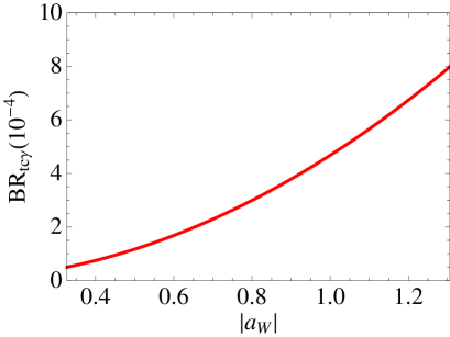
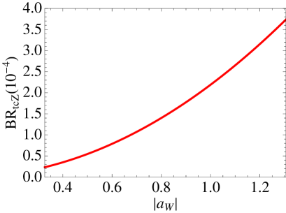
Figure 1: The branching fractions (a) $BR_{tc\gamma}(10^{-4})$, and (b) $BR_{tcZ}(10^{-4})$ plotted as a function of $|a_{W}|$ for $m_{t}=171.3$ GeV, and $\Lambda=1$ TeV. Here $|a_{W}|$ is varied between 0.5 g and 2 g.

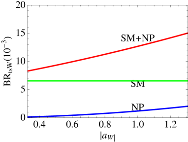
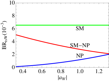
Figure 2: The branching fraction $BR_{tsW}$ plotted as a function of $|a_{W}|$ for $m_{t}=171.3$ GeV, and $\Lambda=1$ TeV. Here $|a_{W}|$ is varied between 0.5 g and 2 g. (a) We assume constructive interference between the SM and NP contributions. (b) We assume destructive interference between the SM and NP contributions.

4 Conclusion

In this paper, we considered rare $b\to sV,V=\gamma,Z$ and $t\to cV,V=\gamma,Z$ decays that arise from the same non-SM physics, or in other words, the same higher dimensional operator corrections to the standard model. The existing constraints from $B$ physics strongly constrain the NP contributions to $t\to cZ(\gamma)$. In certain situation, the constraints from $B$ decays as well as top branching fraction measurements still allow branching ratios for $t\to cZ(\gamma)$ that may be accessible at the LHC.

5 Acknowledgments

The work of A.D was supported by a research grant from the College of Liberal Arts, University of Mississippi.

References

• [1]
• [2] See the heavy flavor averaging group and references therein.
• [3] M. Misiak et al., Phys. Rev. Lett.  98, 022002 (2007) [arXiv:hep-ph/0609232].
• [4] R. Mohanta and A. K. Giri, Phys. Rev.  D 78, 116002 (2008) [arXiv:0812.1077 [hep-ph]].
• [5] J. A. Aguilar-Saavedra, F. J. Botella, G. C. Branco and M. Nebot, Nucl. Phys.  B 706, 204 (2005) [arXiv:hep-ph/0406151].
• [6] C. Amsler et al. (Particle Data Group), Physics Letters B667, 1 (2008) and 2009.
• [7] G. Eilam, J. L. Hewett and A. Soni, Phys. Rev.  D 44, 1473 (1991) [Erratum-ibid.  D 59, 039901 (1999)].
• [8] B. Mele, S. Petrarca and A. Soddu, Phys. Lett.  B 435, 401 (1998) [arXiv:hep-ph/9805498].
• [9] M. Beneke et al., physics,” arXiv:hep-ph/0003033; T. Han, arXiv:0804.3178 [hep-ph]. W. Bernreuther, the LHC,” J.  Phys.  G 35, 083001 (2008) [arXiv:0805.1333 [hep-ph]]; D. Chakraborty, J. Konigsberg and D. L. Rainwater, Part. Sci. 53, 301 (2003) [arXiv:hep-ph/0303092]. J. Carvalho et al. [ATLAS Collaboration], Eur. Phys. J.  C 52, 999 (2007) [arXiv:0712.1127 [hep-ex]]; ATLAS Collaboration, Expected Performance of the ATLAS Experiment, Detector, Trigger and Physics, CERN-OPEN-2008-020, Geneva, 2008, to appear.
• [10] See for example, J. A. Aguilar-Saavedra, flavour-changing neutral interactions: Theoretical expectations and [arXiv:hep-ph/0409342]; T. M. Aliev, O. Cakir and K. O. Ozansoy, Phys. Lett.  B 670, 336 (2009); [arXiv:0809.2327 [hep-ph]]. J. J. Zhang, C. S. Li, J. Gao, H. Zhang, Z. Li, C. P. Yuan and T. C. Yuan, Phys. Rev. Lett.  102, 072001 (2009); [arXiv:0810.3889 [hep-ph]]. M. Frank and I. Turan, supersymmetric model,” Phys.  Rev.  D 72, 035008 (2005) [arXiv:hep-ph/0506197]; C. S. Li, R. J. Oakes and J. M. Yang, in the minimal supersymmetric model,” Phys. Rev. D 49, 293 (1994) [Erratum-ibid.  D 56, 3156 (1997)]; PHRVA,D49,293;G. M. de Divitiis, R. Petronzio and L. Silvestrini, changing top decays in supersymmetric extensions of the standard [arXiv:hep-ph/9704244]; J. L. Lopez, D. V. Nanopoulos and R. Rangarajan, contributions to t –¿ c V,” Phys. Rev.  D 56, 3100 (1997) [arXiv:hep-ph/9702350]. H. Hong-Sheng, littlest Higgs model with (2007) [arXiv:hep-ph/0703067]; G. Eilam, A. Gemintern, T. Han, J. M. Yang and X. Zhang, rare decay t $\rightarrow$ c h in R-parity-violating SUSY,” Phys.  Lett. B 510, 227 (2001) [arXiv:hep-ph/0102037]; PHLTA,B510,227;M. E. Luke and M. J. Savage, top decays,” Phys. Lett.  B 307, 387 (1993) [arXiv:hep-ph/9303249].
• [11] T. Han, R. D. Peccei and X. Zhang, via flavor changing neutral currents at hadron colliders,” Nucl. Phys. B 454, 527 (1995) [arXiv:hep-ph/9506461]. NUPHA,B454,527;
• [12] T. Han, K. Whisnant, B. L. Young and X. Zhang, quark decay via the anomalous coupling $\bar{t}c\gamma$ at hadron [arXiv:hep-ph/9603247].
• [13] T. Han, K. Whisnant, B. L. Young and X. Zhang, Phys. Lett.  B 385, 311 (1996) [arXiv:hep-ph/9606231].
• [14] T. P. Cheng and M. Sher, Phys. Rev.  D 35, 3484 (1987).
• [15] A. Datta and P. J. O’Donnell, Phys. Rev.  D 72, 113002 (2005) [arXiv:hep-ph/0508314].
• [16] A. Datta, Published in Phys.Rev.D78:095004,2008. e-Print: arXiv:0807.0795 [hep-ph]
• [17] X. G. He and G. Valencia, Phys. Lett.  B 680, 72 (2009) [arXiv:0907.4034 [hep-ph]].
• [18] W. Buchmuller and D. Wyler, Nucl. Phys.  B 268, 621 (1986).
• [19] A. Datta and X. Zhang, production Phys. Rev.  D 55, 2530 (1997) [arXiv:hep-ph/9611247].
• [20] P. J. Fox, Z. Ligeti, M. Papucci, G. Perez and M. D. Schwartz, Phys. Rev.  D 78, 054008 (2008) [arXiv:0704.1482 [hep-ph]].
• [21] A. J. Buras, M. Misiak, M. Munz and S. Pokorski, Nucl. Phys.  B 424, 374 (1994) [arXiv:hep-ph/9311345].
• [22] CKMfitter Group, ”http://ckmfitter.in2p3.fr/”