The dynamics of loop formation in a semiflexible polymer

Abstract

The dynamics of loop formation by linear polymer chains has been a topic of several theoretical/experimental studies. Formation of loops and their opening are key processes in many important biological processes. Loop formation in flexible chains has been extensively studied by many groups. However, in the more realistic case of semiflexible polymers, not much results are available. In a recent study (K. P. Santo and K. L. Sebastian, Phys. Rev. E, 73, 031293 (2006)), we investigated opening dynamics of semiflexible loops in the short chain limit and presented results for opening rates as a function of the length of the chain. We presented an approximate model for a semiflexible polymer in the rod limit, based on a semiclassical expansion of the bending energy of the chain. The model provided an easy way to describe the dynamics. In this paper, using this model, we investigate the reverse process, i.e., the loop formation dynamics of a semiflexible polymer chain by describing the process as a diffusion-controlled reaction. We make use of the “closure approximation” of Wilemski and Fixmann (G. Wilemski and M. Fixmann, J. Chem. Phys., 60, 878 (1974)), in which a sink function is used to represent the reaction. We perform a detailed multidimensional analysis of the problem and calculate closing times for a semiflexible chain. We show that for short chains, the loop formation time $\tau$ decreases with the contour length of the polymer. But for longer chains, it increases with length obeying a power law and so it has a minimum at an intermediate length.  In terms of dimensionless variables, the closing time is found to be given by $\tau\sim L^{n}\exp(\mathrm{const.}/L)$, where $n=4.5-6$. The minimum loop formation time occurs at a length  $L_{m}$ of about $2.2-2.4$. These are, indeed, the results that are physically expected, but a multidimensional analysis leading to these results does not seem to exist in the literature so far.

I Introduction

In a previous paper Santo and Sebastian (2006), the dynamics of opening of a weak bond between the two ends of a semiflexible polymer chain was considered in detail. An approximate model for a stiff polymer ring in the rod limit, based on a “semiclassical” method was developed. This model, though approximate, was found to provide an easy approach to describe the dynamics of a worm-like polymer chain in the rod limit. In Ref. Santo and Sebastian (2006), we used the model to analyze the dynamics of opening and to calculate the rates of opening as a function of length in the short chain limit. Here in this paper, we analyze the dynamics of loop formation.

The closing dynamics of polymer chains has been studied extensively, being the key process in important biological functions, such as control of gene expression Rippe (2001); Rippe et al. (1995), DNA replication Jun and Bechhoefer (2003) and protein folding. Experimental studies on loop formation involve monitoring the dynamics of DNA hairpins Bonnet et al. (1998); Wallace et al. (2001); Goddard et al. (2000); Ansari et al. (2001); Shen et al. (2001) and small peptides Lapidus et al. (2002); Hagen et al. (2002); Lapidus et al. (2000, 2001), using fluorescence spectroscopic techniques. Several theoretical approaches are available for analyzing loop formation of a flexible chain. Using the formalism of Wilemski and Fixman (WL) Wilemski and Fixman (1974) for diffusion controlled reactions, the closing time $\tau$ for a flexible chain was calculated by Doi Doi (1975) and was found to vary as, $\tau\sim L^{2}$. In another important approach, Szabo, Schulten and Schulten (SSS) Szabo et al. (1980) calculated the mean first passage time for closing for a gaussian chain and found $\tau\sim L^{3/2}$. The two approaches have been analyzed by recent simulations Srinivas et al. (2002); Pastor et al. (1996). But real polymers such as DNA, RNA and proteins are not flexible and hence, it is more important to understand the closing dynamics of stiff chains. Unfortunately, in this case, only simple, approximate approaches Wilhelm and Frey (1996); Chirikjian and Wang (2000); Winkler et al. (1994); Freed (1971); Harris and Hearst (1966); Saito et al. (1967) are available in the literature so far. Since worm-like chains are represented by differentiable curves, one has to incorporate the constraint $|\mathbf{u}(s)|=1$ and this has been a problem in dealing with semiflexible polymers. Yamakawa and Stockmayer Yamakawa and Stockmayer (1972) and Shimada and Yamakawa Shimada and Yamakava (1984) have calculated the static ring closure probabilities for worm-like chains and helical worm-like chains. According to their analysis, the ring closure probability for a worm-like chain has the form, $G(\mathbf{0};L)=896.32(l_{p}/L)^{5}\exp(-14.054l_{p}/L+0.246L/l_{p}),$ where $l_{p}$ is the persistence length of the chain. An approximate treatment that leads to the end-to-end probability distribution for semiflexible polymers has been given by Winkler et. al Winkler et al. (1994) and using their approach, the closing dynamics has been analyzed recently by Cherayil and Dua Dua and Cherayil (2002). They find that the closing time $\tau\sim L^{\nu}$, where $\nu$ is in the range $2.2$ to $2.4$. In an interesting paper, Jun. et. al Jun et al. (2003) showed that the closing time should decrease with length in the short chain limit and then increase with length for longer chains. Hence, the closing time has a minimum at an intermediate length. The reason for this behavior is that, for short chains, the bending energy contributes significantly to the activation energy for the process. Thus the activation energy $\sim{\mathrm{const.}}/L$ and therefore the closing time $\tau\sim\exp({\mathrm{const.}}/L)$. For longer chains, the free energy barrier for closing is due to the configurational entropy and hence, $\tau$ obeys a power law. Jun et. al Jun et al. (2003) have followed an approximate one dimensional Kramers approach to reproduce this behavior and obtain the minimum of closing time at a length $L_{m}=3.4l_{p}$, where $l_{p}$ is the persistence length of the chain. Monte Carlo simulations by Chen et.al Chen et al. (2004) lead to $L_{m}=2.85l_{p}$. See also the paper by Ranjith et al Ranjith et al. (2005).

In Ref. Santo and Sebastian (2006), we analyzed the opening dynamics of a semiflexible polymer ring formed by a weak bond between the ends. We developed a model that describe the polymer near the ring configuration, using a semiclassical expansion of the bending energy of the chain. The model, though approximate, provided an easy way to analyze the dynamics. Using this model, we calculated the opening rates as function of the contour length of the chain. The formalism presented in Ref.Santo and Sebastian (2006), took into account of the inextensibility constraint, $|\mathbf{u}(s)|=1$ for semiflexible chains rigourously. The conformations of the chain can be mapped onto the paths of a Brownian particle on a unit sphere. We performed a semiclassical expansion about the most probable path assuming that the fluctuations about the most probable path are small. For the ring, we took most probable path to be the great circle on the sphere. This is again an approximation, as the minimum energy configuration for a semiflexible polymer loop does not correspond to the great circle. However, as described in Ref. Santo and Sebastian (2006), it led to minimum energy values very close to exact results by Yamakawa and Stockmayer Yamakawa and Stockmayer (1972) and the approximation scheme by Kulic and Schiessel Kulic and Schiessel (2003). Once the ends of a semiflexible polymer are brought together, they can separate in any of the three directions in space. Our analysis showed that two of the three directions in space are unstable, while one direction is stable. If one considers the ring to be in the $XY$-plane, with its ends meeting on the $Y$ axis, then the motion that leads to separation along the $Y$ direction is stable, while the motions lead to separation along $X$ or $Z$ direction are unstable. The nature of instabilities along the $X$ and $Z$ directions are different. Hence, near the ring, the three directions in space are non-equivalent for a semiflexible polymer and are governed by different energetics (see Sec. III.2). One may also perform the expansion near the rod configuration by expanding about the straight rod. On the unit sphere the straight rod corresponds to a point and unlike the great circle this is an exact minimum energy configuration (see Sec. III).

In this paper, we present a detailed multidimensional analysis of the dynamics of loop formation in semiflexible chains. We make use of the approximation scheme developed in Ref. Santo and Sebastian (2006). Following Wilemski and Fixman Wilemski and Fixman (1974), the looping is described as a diffusion-controlled reaction. In the WF theory, the effect of the reaction is incorporated into the model using a sink function. In special cases, exact analytical results are possible for a delta function sink Bicout and Szabo (1997); Sebastian (1992); Debnath et al. (2006). But for an arbitrary sink, and multidimensional dynamics, this is not possible. For such cases, WF suggested an approximation known as the “closure” approximation. In this, the diffusion limited life-time of the process is expressed in terms of a sink-sink correlation function and the essential step for finding the loop formation time is to calculate this sink-sink correlation function. For this, we need to know the time-dependent Green’s function of the chain and the equilibrium probability distribution. We therefore derive the time-dependent multidimensional Green’s function of the semiflexible polymer near the loop configuration by performing a normal mode analysis. This Green’s function is then used to find the sink-sink correlation function for a Gaussian sink and the closing time. We find that the closing time $\tau\sim(L/l_{p})^{n}\exp(Al_{p}/L)$, The exponent $n=4.5$ - $6$. $\tau$ is found to be a minimum at a length $L_{m}\simeq$ $2.2-2.4l_{p}$ which has to be compared with the value $3.4l_{p}$ obtained in Ref. Jun et al. (2003) and $2.85l_{p}$ of Ref. Chen et al. (2004). We find $L_{m}$ to be weakly dependent on the range of the interaction between the ends. Thus, our analysis leads to results that are physically expected. It is worth mentioning that a multidimensional analysis leading to these results does not seem to exist in the literature so far.  We also calculate the loop formation probability $G(\mathbf{0};L)$ and find that our method leads to the correct behavior, i.e., $G(\mathbf{0};L)\sim L^{-5}\exp(-\mathrm{const.}/L)$, thus showing that the procedure reproduces the previous results for this quantity Shimada and Yamakava (1984).

The paper is organized as follows: In Sec.II, we give a summary of the WF theory for diffusion controlled reactions and the “closure” approximation. In Sec. III, the semiclassical approximation scheme for bending energy of a semiflexible polymer is briefly outlined. The time dependent Green’s function of the polymer is derived though a normal mode analysis near the loop configuration in Sec. IV. The approximate probability distribution of the chain is given in Sec. IV. In Sec. VI.1, we calculate the sink-sink correlation function for a Gaussian sink and the closing time. In Sec. VI.2, we give numerical results. Summary and conclusions are given in Sec. VII.

II The “closure” approximation

In this section, we summarize the theory of diffusion-controlled intra-chain reactions of polymers developed by Wilemski and Fixman Wilemski and Fixman (1974) and their “ closure” approximation for an arbitrary sink function. The dynamics of a single polymer chain in a viscous environment is governed by the diffusion equation,

$$\frac{\partial P}{\partial t}+{\hat{D}}P=0,$$ (1)

where ${\hat{D}}$ is the diffusion operator for the chain. If the chain is represented by $N+1$ beads with position vectors represented by $\mathbf{r}=(\mathbf{r}_{1},\mathbf{r}_{2},....\mathbf{r}_{N+1})$, then the general form of the diffusion operator is given by

$${\hat{D}}=D\sum\limits_{i=1}^{N+1}\nabla_{i}.(\nabla_{i}+(k_{B}T)^{-1}\mathbf{F}_{i}).$$ (2)

$D=k_{B}T/\xi$, is the diffusion coefficient of the segments and $\xi$ is the friction coefficient of the segments. $\mathbf{F}_{i}=\nabla_{i}U$, where $U$ is the potential energy of the chain. Eq. (1) may be solved to obtain the equilibrium distribution $P_{eq}$ of the chain, which is time independent. But if the chain has reactive ends, they can react and form a loop when they come sufficiently close and hence the probability distribution of an open chain will decay in time. In such a case, one may solve Eq. (1) with appropriate boundary conditions. An alternate approach to the same problem is to introduce a sink function into the equation for $P(\mathbf{r},t)$ as done by Wilemski and Fixman Wilemski and Fixman (1974). Then the reaction-diffusion equation that governs the dynamics of a polymer chain with reactive ends is

$$\frac{\partial P}{\partial t}+{\hat{D}}P=-k_{r}\mathcal{S}(\mathbf{r})P,$$ (3)

where $P$ is the distribution function of the open polymer chain and $k_{r}$ is the strength of the sink function. $k_{r}$ determines the rate at which the reaction occurs when the ends are sufficiently close. $\mathcal{S}$ is the sink function and is a function of $\mathbf{r}_{1},\mathbf{r}_{2},...\mathbf{r}_{N+1}$. Integrating Eq. (3) over all the coordinates $\mathbf{r}$ we get

$$\frac{dP_{s}(t)}{dt}=-k_{r}v(t),$$ (4)

where

$$v(t)=\int d\mathbf{r}\mathcal{S}(\mathbf{r})P(\mathbf{r},t)$$ (5)

and

$$P_{s}(t)=\int d\mathbf{r}P(\mathbf{r},t)$$ (6)

is the survival probability. The function $\mathcal{S}$ can be any suitable function, but is usually taken to be a delta function or a gaussian. Eq. (3) can be solved exactly only in one dimension for a delta function sink or a quadratic sink (see references Bicout and Szabo (1997); Sebastian (1992); Debnath et al. (2006) , and the references therein). Therefore, WF introduced the assumption that $P(\mathbf{r},t)$ may be approximated as

$$P(\mathbf{r},t)=P_{eq}(\mathbf{r})\nu(t),$$ (7)

where

$$\nu(t)=\frac{v(t)}{v_{eq}}$$ (8)

with

$$v_{eq}=\int d\mathbf{r}\mathcal{S}(\mathbf{r})P_{eq}(\mathbf{r}).$$ (9)

This is referred to as the “closure” approximation. The average time of closing is the integral of the survival probability and is given by

$$\tau=\int\limits_{0}^{\infty}P_{s}(t)dt=\tilde{P_{s}}(0),$$ (10)

where $\tilde{P_{s}}(s)$ is the Laplace transform of $P_{s}(t)$. $\tau$ is also expressed in terms of a sink-sink correlation function and in the diffusion-limited ($k_{r}\rightarrow\infty$) limit, it is given by Wilemski and Fixman (1974)

$$\tau=\int\limits_{0}^{\infty}\left(\frac{\mathcal{D}(t)}{v_{eq}^{2}}-1\right)dt.$$ (11)

$\mathcal{D}(t)$ is the sink-sink correlation function defined by

$$\mathcal{D}(t)=\int d\mathbf{r}\int d\mathbf{r}^{\prime}\mathcal{S}(\mathbf{r})G_{0}(\mathbf{r},\mathbf{r}^{\prime};t)\mathcal{S}(\mathbf{r}^{\prime})P_{eq}(\mathbf{r}^{\prime}),$$ (12)

where $G_{0}(\mathbf{r},\mathbf{r}^{\prime};t)$ is the Green’s function for the diffusive motion of the chain in the absence of the sink. Eq. (11) was obtained by WF Wilemski and Fixman (1974). Note that $\mathcal{D}(\infty)=v_{eq}^{2}$. To calculate $\mathcal{D}(t)$, one needs to know $G_{0}(\mathbf{r},\mathbf{r}^{\prime};t)$ and $P_{eq}(\mathbf{r})$ and these will be calculated in the following sections. We shall take $\mathcal{S}(\mathbf{r})$ to be a Gaussian, given by

$$\mathcal{S}(\mathbf{r})\equiv\mathcal{S}(\mathbf{R})=\mathcal{S}_{x}(R_{x})\mathcal{S}_{y}(R_{y})\mathcal{S}_{z}(R_{z}),$$ (13)

where $\mathbf{R}$ is the end to end vector for the chain and

$$\mathcal{S}_{i}(R_{i})=e^{-R_{i}^{2}/(2\eta^{2})}/(\sqrt{2\pi}\ \eta),\text{ \ }i=x,y\text{ \ or }z.$$ (14)

$\eta$ is the width of the Gaussian sink.

III The semi-classical Approximation scheme for the Bending Energy

In Ref.Santo and Sebastian (2006), we introduced an approximation scheme for the bending energy of a semiflexible polymer ring, which is based on a “semiclassical” expansion. In this section, we give a brief account of the approach. A semiflexible polymer is usually considered as a continuous, inextensible space curve represented by the position vector $\mathbf{r}(s)$, where $s$ is the arc-length parameter. The bending energy of the chain is given by

$$E_{bend}=\frac{\kappa}{2}\int\limits_{0}^{L}\left(\frac{\partial^{2}\mathbf{r}(s)}{\partial s^{2}}\right)^{2}ds.$$ (15)

$\kappa$ is the bending rigidity. Since the curve is differentiable, one has the constraint,

$$|\mathbf{u}(s)|=1,$$ (16)

where $\mathbf{u}(s)=\partial\mathbf{r}(s)/\partial s$, the tangent vector at the point $s$. The partition function of the semiflexible polymer is the functional integral over the conformations represented by $\mathbf{r}(s)$,

$$Z=\int\mathbf{Dr}(s)\exp\left(\frac{-E_{bend}[\mathbf{r}(s)]}{k_{B}T}\right).$$ (17)

This functional integral has to be performed with the constraint of Eq. (16). However, incorporating this constraint has been a problem in dealing with semiflexible polymers. In Ref. Santo and Sebastian (2006), we wrote the partition function as an integral over ${\mathbf{u}}(s)$,

$$Z=\int\mathbf{Du}(s)\exp\left(\frac{-E_{bend}[\mathbf{u}(s)]}{k_{B}T}\right).$$ (18)

and represented $\mathbf{u}(s)$ in angle coordinates

$$\mathbf{u}(s)=\mathbf{i}\sin\theta(s)\cos\phi(s)+\mathbf{j}\sin\theta(s)\sin\phi(s)+\mathbf{k}\cos\theta(s).$$ (19)

Since the magnitude of the tangent vector is one, the conformations of the semiflexible polymer can be mapped onto the trajectories of a Brownian particle over a unit sphere (Fig.1).

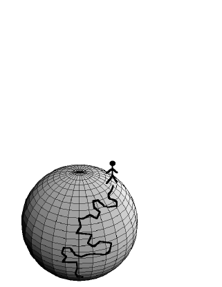
Figure 1: The conformations of a semiflexible polymer may be mapped onto the paths of a Brownian particle on the surface of a unit sphere. The circular ring polymer with the tangent vectors at the ends joining smoothly corresponds to the great circle on the unit sphere.

The bending energy of the chain is then written in terms of the angles $\theta$ and $\phi$ as

$$E_{bend}=\frac{\kappa}{2}\int\limits_{0}^{L}ds\left\{\left(\frac{d\theta(s)}{ds}\right)^{2}+\sin^{2}\theta(s)\left(\frac{d\phi(s)}{ds}\right)^{2}\right\}$$ (20)

and the partition function is written as a path integral in spherical polar coordinates

$$Z_{loop}=\int D\theta(s)\int D\phi(s)\exp\left(-\frac{E_{bend}[\theta(s),\phi(s)]}{k_{B}T}\right).$$ (21)

This path integral has not been evaluated in a closed form. In Ref. Santo and Sebastian (2006), we have used a semiclassical expansion of the bending energy, to evaluate the above partition function approximately.

III.1 Bending energy of the loop: expansion about the great circle

To perform a semiclassical expansion of the bending energy of the semiflexible polymer near the ring configuration, we take the most important path to be the great circle on the unit sphere (Fig. 1). The great circle corresponds to a ring with the tangents smoothly joined. However, the minimum energy configuration of a rod-like polymer whose ends are brought together to form a loop would not have its tangents joining smoothly and therefore does not correspond to a great circle Yamakawa and Stockmayer (1972). Hence, our approach is approximate but has the advantage that it provides an easy way to study the dynamics.  On the other hand, if one is interested in covalent bond formation, in which directionality of the bond is important, then the great circle is the appropriate starting point.

The position vector of the polymer may be found by inverting the definition of the tangent vector ${\mathbf{u}}(s)=\partial{\mathbf{r}}(s)/\partial s$,

$$\mathbf{r}(s)=\mathbf{r}_{cm}-\frac{1}{L}\int_{0}^{L}ds\int_{0}^{s}ds_{1}\mathbf{u}(s_{1})+\int_{0}^{s}ds_{1}\mathbf{u}(s_{1}),$$ (22)

where $\mathbf{r}_{cm}$ denotes the position vector of the center of mass of the ring polymer. The great circle is chosen to lie in the XY plane of a Cartesian coordinate system, with any point on it represented by the coordinates, $[\theta(s),\phi(s)]=\left[\pi/2,2\pi s/L\right]$. The position vector of the circular ring polymer that corresponds to the great circle may be found using Eq. (22) and is given by

$$\mathbf{r}_{GC}(s)=\frac{L}{2\pi}\left[\mathbf{i}\sin\left(\frac{2\pi s}{L}\right)-\mathbf{j}\cos\left(\frac{2\pi s}{L}\right)\right].$$ (23)

This curve represents one end of the polymer lying in the XY-plane starting at $\frac{-L}{2\pi}$ on the negative Y axis, going around the Z axis along a circle of radius $\frac{L}{2\pi}$, coming back to the same point after traversing a circle of radius $\frac{L}{2\pi}$. The fluctuations about this path are taken into account by letting

$$[\theta(s),\phi(s)]=\left[\frac{\pi}{2}+\delta\theta(s),\frac{2\pi s}{L}+\delta\phi(s)\right],$$ (24)

where $\delta\theta(s)$ and $\delta\phi(s)$ represent the deviations from the extremum path on the unit sphere expressed in terms of angles. Expanding the bending energy of Eq. (20) correct up to second order in the fluctuations $\delta\theta(s)$ and $\delta\phi(s)$ gives

$$\begin{array}[]{l}E_{bend}=\frac{\kappa}{2}\int\limits_{0}^{L}ds\left\{\left(\frac{d\delta\theta(s)}{ds}\right)^{2}+\left(\frac{2\pi}{L}+\frac{d\delta\phi(s)}{ds}\right)^{2}-\left(\frac{2\pi}{L}\right)^{2}\delta\theta^{2}(s)\right\}.\end{array}$$ (25)

We expect this expansion to be a valid approximation near the ring configuration, if the deviations from the circular configuration is small.

We expand fluctuations as

$$\delta\phi(s)=\sum\limits_{n=0}^{\infty}\delta\phi_{n}\cos\left(\frac{n\pi s}{L}\right)$$ (26)

and

$$\delta\theta(s)=\sum\limits_{n=0}^{\infty}\delta\theta_{n}\cos\left(\frac{n\pi s}{L}\right).$$ (27)

In terms of these modes, the bending energy of the chain is given by

$$\begin{array}[]{c}E_{bend}=\frac{\kappa}{4L}\{-8\pi^{2}\delta\theta_{0}^{2}+\sum\limits_{n=1}^{\infty}(n^{2}-4)\pi^{2}{\delta\theta_{n}}^{2}+\sum\limits_{n,odd}n^{2}\pi^{2}\left(\delta\phi_{n}-\frac{8}{n^{2}\pi}\right)^{2}+\sum\limits_{n,even}n^{2}\pi^{2}\delta\phi_{n}^{2}\}.\end{array}$$ (28)

In the above, the bending energy is independent of the modes $\delta\theta_{2}$ and $\delta\phi_{0}$. These give two of the three rotational degrees of freedom of the ring polymer in space. $\delta\phi_{0}$ corresponds to the rotation about the $Z$ axis, while $\delta\theta_{2}$ corresponds to rotation of the ring about X axis. A fluctuation of the form $\delta\theta_{2s}\sin(2\pi s/L)$ leads to rotation about $Y$ axis. The value of $\delta\theta_{2s}$ (the amount of of rotation contained) in an arbitrary $\delta\theta(s)$ may be found from

$$\delta\theta_{2s}=\frac{2}{L}\int\limits_{0}^{L}\delta\theta(s)\sin\left(\frac{2\pi s}{L}\right).$$ (29)

Using Eq. (27) in Eq. (29), one gets

$$\delta\theta_{2s}=2\sum\limits_{n}a_{n}\delta\theta_{n},$$ (30)

where

$$\begin{array}[]{c}a_{n}=\frac{-4}{(n^{2}-4)\pi},\ \mathrm{\ if\ n\ is\ odd}\\ =0,\ \mathrm{\ if\ n\ is\ even}.\end{array}$$ (31)

While evaluating the partition function one must avoid integrating over the rotational modes, since within our approximation scheme, these modes would cause the partition function to diverge. One can remove these rotational degrees of freedom by inserting the product of delta functions $\delta(\delta\phi_{0})\delta(\delta\theta_{2})\delta(\delta\theta_{2s})$ to the functional integral and then taking the contribution of the rotational modes to the partition function into account by explicitly putting in the factor $8\pi^{2}$. Then the probability for the loop formation is given by

$$\begin{array}[]{c}G(\mathbf{0,}L\mathbf{|0})=\frac{8\pi^{2}}{Z_{R}}\int D\delta\theta(s)\int D\delta\phi(s)\exp\left(-\frac{E_{bend}[\delta\theta(s),\delta\phi(s)]}{k_{B}T}\right)\delta(\delta\phi_{0})\delta(\delta\theta_{2})\delta(\delta\theta_{2s})\delta(\mathbf{R}).\end{array}$$ (32)

$\mathbf{R}$ is the end to end vector for the polymer chain and $Z_{R}$ is the partition function for the polymer, approximated by that appropriate for a semi-flexible rod of length $L$ (see Eq. (72)).

III.2 The asymmetry in the three directions of motion at the ring geometry

In Ref. Santo and Sebastian (2006), we derived the expression for the end-to-end vector $\mathbf{R}$, by expanding the components of $\mathbf{u}(s)$ as a Taylor series up to first order, which is

$$\mathbf{R}=L\left(\mathbf{i}\sum\limits_{n\ odd}^{\infty}a_{n}\delta\phi_{n}-\mathbf{j}\frac{\delta\phi_{2}}{2}+\mathbf{k}\delta\theta_{0}\right).$$ (33)

The components of ${\mathbf{R}}$ are given by, $R_{x}=L\sum_{n,odd}^{\infty}a_{n}\delta\phi_{n}$, $R_{y}=-\frac{L}{2}\delta\phi_{2}$ and $R_{z}=L\delta\theta_{0}$. Thus $R_{x}$ can be changed by varying the value of $\delta\phi_{n}$s for odd $n$. It can be easily seen from Eq. (28), that increasing $\delta\phi_{n}$s with $n$ odd decreases the bending energy of the chain towards a minimum at $\delta\phi_{n}=8/n^{2}\pi$ ($n$ odd). Using this value for $\delta\phi_{n}$ ($n$ odd ) one gets

$$R_{x}=L\sum\limits_{n,odd}^{\infty}a_{n}\frac{8}{n^{2}\pi}=L,$$ (34)

since $\sum_{n,odd}^{\infty}a_{n}/n^{2}=\pi/8$. Hence, this value of $\delta\phi_{n}$ corresponds to a rod lying along the $X$ axis. Therefore, the ring is unstable along $R_{x}$ and the bending energy along this direction has the minimum at $R_{x}=L$. Also, increasing $\delta\theta_{0}$ decreases the bending energy and therefore, $R_{z}$ is also unstable. This is because when $R_{z}$ is increased the ring changes into a helix, which has less curvature and therefore less bending energy. (Note that we do not take torsional energies into account in this analysis). But unlike $R_{x}=0$, $R_{z}=0$ is a maximum. It should be noted that $R_{z}=L$ corresponds to the rod and should be a minimum, but our analysis does not reproduce this. So, the instability along $R_{z}$ is only near the ring, where our analysis is valid. Unlike $R_{x}$ and $R_{z}$, $R_{y}$ is stable, since the bending energy of the ring increases when $\delta\phi_{2}$ is increased. Thus, the motion in $R_{x}$, $R_{y}$ and $R_{z}$ directions are energetically different.

III.3 Bending energy of the rod

For a semiflexible chain, the minimum energy configuration is the rod. On the unit sphere representing the tangents this means that the random walker stays at the starting point. We take this point to be $(\theta(s),\phi(s))=(\pi/2,0)$, which corresponds to the rod lying along the X axis. Unlike the great circle, the straight rod is an exact minimum energy configuration. In this case, the fluctuations can be incorporated by letting

$$[\theta(s),\phi(s)]=\left[\frac{\pi}{2}+\delta\theta(s),\delta\phi(s)\right].$$ (35)

The bending energy of the rod correct up to the second order in fluctuations is then given by

$$E_{rod}=\frac{\kappa}{2}\int\limits_{0}^{L}\left\{\left(\frac{d\delta\theta(s)}{ds}\right)^{2}+\left(\frac{\delta\phi(s)}{ds}\right)^{2}\right\}ds.$$ (36)

Using the expansions Eq. (26) and Eq. (27), one gets

$$E_{rod}=\frac{\kappa}{4L}\sum\limits_{n=0}^{2\mathcal{N}}n^{2}\pi^{2}(\delta\theta_{n}^{2}+\delta\phi_{n}^{2}).$$ (37)

Unlike the ring, the rod has only two rotational degrees of freedom. From Eq. (37), it follows that these are the modes $\delta\phi_{0}$ and $\delta\theta_{0}$. For the convenience of bookkeeping, we assume that the number of $\delta\phi_{n}$ and $\delta\theta_{n}$ modes and both equal to $2\mathcal{N}$, with $n=0,1,2...(2\mathcal{N}-1)$.  Thus there are $4\mathcal{N}$ modes in total, with $\mathcal{N}\rightarrow\infty$.

IV The normal coordinates and the Green’s function

In this section, we use the approximation scheme for the bending energy described in Sec. III.1, to analyze the dynamics of loop formation. The approximation of Eq. (28) is valid only near the most important path corresponding to the loop, since the fluctuations about this path are assumed to be small. The time evolution of the chain may be described by the multidimensional Green’s function $G_{0}(\mathbf{\Psi},t|\mathbf{\Psi}_{0})$, where $\mathbf{\Psi}^{{\dagger}}=(\mathbf{\Phi}^{{\dagger}},\mathbf{\Theta}^{{\dagger}})$ with $\mathbf{\Phi}^{{\dagger}}=(\delta\phi_{0},\delta\phi_{2},..\delta\phi_{2\mathcal{N}-2},\delta\phi_{1},\delta\phi_{3},..\delta\phi_{2\mathcal{N}-1})$ (note that we have separated out the even and odd modes) and $\mathbf{\Theta}^{{\dagger}}=(\delta\theta_{0},\delta\theta_{2},..\delta\theta_{2\mathcal{N}-2},\delta\theta_{1},\delta\theta_{3},..\delta\theta_{2\mathcal{N}-1})$. The superscript $\dagger$ stands for transpose.  The bending energy of the polymer near the ring configuration is given by Eq. (28) and therefore, $G_{0}$ for configurations close to the ring may be obtained by solving the corresponding equations of motion. Because of our approximation for the energy, the Green’s function so obtained is not valid for large $\mathbf{R}$. Yet, the sink-sink correlation function, $\mathcal{D}(t)$ of Eq. (12), may still be evaluated, since the sink function $\mathcal{S}(\mathbf{R})$ is nonzero only for very small values of $\mathbf{R}$. This of course, is approximate. The function $G_{0}$ may be found by solving the equations of motion of the polymer near the loop configuration. The angle coordinates, $\mathbf{\Psi}$ are not normal coordinates, since the kinetic energy of the chain has terms that couple these (see Appendix A). As a result, the equations of motion of the chain in terms of them are coupled. This coupling may be avoided by working with the normal modes, which may be found by solving the corresponding eigenvalue problem (Eq. (46)). Then the dynamics of the chain can be reduced to the dynamics of a particle in a multidimensional harmonic potential. The Green’s function $G_{0}$ is obtained as a product of the one-dimensional Green’s functions corresponding to each of the normal modes.

IV.1 The Hamiltonian and the normal modes

The kinetic energy of the polymer in the center of mass frame is

$$T=\frac{\rho}{2}\int\limits_{0}^{L}\left[\frac{\partial\mathbf{r}(s)}{\partial t}\right]^{2}dt,$$ (38)

where $\mathbf{r}(s)$ is given by Eq. (22). Near the rod ring configuration, the kinetic energy of the polymer in terms of the Fourier modes $\delta\theta_{n}$ and $\delta\phi_{n}$ may be written as

$$\begin{array}[]{c}T_{R}=\frac{\rho L^{3}}{2}\overset{.}{\mathbf{\Psi}}_{R}^{{\dagger}}\mathcal{T}_{R}\overset{.}{\mathbf{\Psi}_{R}}.\end{array}$$ (39)

The dot in $\overset{.}{\mathbf{\Psi}_{R}}$ represents differentiation with respect to time. The subscripts $R(L)$ in $\mathbf{\Psi}_{R}$($\mathbf{\Psi}_{L}$) are used to indicate that these are deviations measured from values appropriate for the rod (loop) geometry. $\ \mathcal{T}_{R}\mathbf{\ }$is the kinetic energy matrix appropriate near the rod configuration.  It has a block diagonal structure, having no matrices connecting the $\theta$ and $\phi$ modes.  Even within the $\theta$ and $\phi$ modes, odd and even modes are decoupled.  Hence $\mathcal{T}_{R}$ may be written as

$$\mathcal{T}_{R}=\left[\begin{array}[]{cccc}\mathbf{T}_{R}^{\phi e}&\mathbf{0}&\mathbf{0}&\mathbf{0}\\ \mathbf{0}&\mathbf{T}_{R}^{\phi o}&\mathbf{0}&\mathbf{0}\\ \mathbf{0}&\mathbf{0}&\mathbf{T}_{R}^{\theta e}&\mathbf{0}\\ \mathbf{0}&\mathbf{0}&\mathbf{0}&\mathbf{T}_{R}^{\theta e}\end{array}\right].$$

Detailed structures of the $\mathbf{T}$ matrices is given in Appendix A. In a similar fashion, near the loop configuration the kinetic energy is given by

$$\begin{array}[]{c}T_{L}=\frac{\rho L^{3}}{2}\overset{.}{\mathbf{\Psi}}_{L}^{{\dagger}}\mathcal{T}_{L}\overset{.}{\mathbf{\Psi}_{L}}.\end{array}$$ (40)

The angles $\overset{.}{\mathbf{\Psi}}_{L}^{{\dagger}}=$ $(\mathbf{\Phi}_{L}^{{\dagger}},\mathbf{\Theta}^{{\dagger}})$ with $\mathbf{\Phi}_{L}^{{\dagger}}=(\delta\phi_{0},\delta\phi_{2},..\delta\phi_{2\mathcal{N}-2},\delta\phi_{1}^{{}^{\prime}},\delta\phi_{3}^{{}^{\prime}},..\delta\phi_{2\mathcal{N}-1}^{\prime})$, where $\delta\phi_{n}^{{}^{\prime}}=\delta\phi_{n}-8/(n^{2}\pi).$  Like $\mathcal{T}_{R},$ $\mathcal{T}_{L}$ too has a block diagonal structure, with the blocks given by the matrices $\mathbf{T}_{L}^{\phi e},\mathbf{T}_{L}^{\phi o},\mathbf{T}_{L}^{\theta e}$ and $\mathbf{T}_{L}^{\theta o}$.  The forms of these too are given in Appendix A. Note that these matrices have no length ($L)$ dependence. It is found that (see Appendix A) the modes of odd and even $n$ decouple. One may rewrite Eq. (28) as

$$\begin{array}[]{c}E_{bend}=\frac{\kappa}{4L}\left[-8\pi^{2}\delta\theta_{0}^{2}+\sum\limits_{n\ even}(n^{2}-4)\pi^{2}{\delta\theta_{n}}^{2}\right]+\\ \frac{\kappa}{4L}\left[\sum\limits_{n,odd}n^{2}\pi^{2}\left(\delta\phi_{n}^{\prime}\right)^{2}+\sum\limits_{n,even}n^{2}\pi^{2}\delta\phi_{n}^{2}\right].\end{array}$$ (41)

or as

$$E_{bend}=\frac{\kappa}{2L}\mathbf{\Psi}_{L}^{{\dagger}}\mathcal{V}_{L}\mathbf{\Psi}_{L}.$$ (42)

Thus the total energy of the polymer molecule near the loop configuration is

$$E=\frac{\rho L^{3}}{2}\overset{.}{\mathbf{\Psi}}_{L}^{{\dagger}}\mathcal{T}_{L}\overset{.}{\mathbf{\Psi}_{L}}+\frac{\kappa}{2L}\mathbf{\Psi}_{L}^{{\dagger}}\mathcal{V}_{L}\mathbf{\Psi}_{L}.$$ (43)

Like $\mathcal{T}_{L}$, $\mathcal{V}_{L}$ too are block diagonal.  The matrices of which $\mathcal{V}_{L}$ is composed of are $\mathbf{V}_{L}^{\phi e},\mathbf{V}_{L}^{\phi o},\mathbf{V}_{L}^{\theta e}$ and $\mathbf{V}_{L}^{\theta o}.$  Each one of them is diagonal and have matrix elements given by $(\mathbf{V}_{L}^{\phi o})_{nm}=\delta_{mn}n^{2}\pi^{2}/2=(\mathbf{V}_{L}^{\phi e})_{nm}$; $(\mathbf{V}_{1}^{\theta})_{00}=-4\pi^{2}$ and all other matrix elements being given by $(\mathbf{V}_{L}^{\theta})_{nm}=\delta_{mn}(n^{2}-4)\pi^{2}/2$.

We will choose the sink function $\mathcal{S}(\mathbf{r})$ as a function only of the end-to-end vector $\mathbf{R}$ (see next section). The dynamics of the closing process must be unaffected by the spatial rotations of the polymer. Hence, the sink-sink correlation function, $\mathcal{D}(t)$ of Eq. (12) is independent of the rotational modes $\delta\phi_{0},\delta\theta_{2}$ and $\delta\theta_{2s}$. From Eq. (33) it follows that $\delta\theta_{n}$ modes with odd $n$ do not contribute to the end-to-end separation $\mathbf{R}$ of the polymer. As $\mathbf{R}$ has no dependence on the odd $\delta\theta_{n}$ modes, they are irrelevant for the dynamics of closing process.

We define $\mathbf{Y}$ by

$$\mathcal{T}^{1/2}\mathbf{\Psi}_{L}=\mathcal{U}\mathbf{Y,}$$ (44)

where $\mathcal{U}$ is to be defined below. Then the energy becomes

$$E=\frac{\rho L^{3}}{2}\overset{.}{\mathbf{Y}}^{{\dagger}}\mathcal{U^{{\dagger}}U}\overset{.}{\mathbf{Y}}+\frac{\kappa}{2L}\mathbf{Y}^{{\dagger}}\mathcal{U^{{\dagger}}\mathcal{T}}^{-1/2}\mathcal{\mathcal{V}}_{L}\mathcal{\mathcal{\mathcal{T}}}^{-1/2}\mathcal{U}\mathbf{Y.}$$ (45)

Taking $\mathcal{U}$ to be a unitary matrix, which diagonalizes $\mathcal{\mathcal{T}}^{-1/2}\mathcal{\mathcal{V}}_{L}\mathcal{\mathcal{\mathcal{T}}}$ ^-1/2 to give the diagonal matrix $\mathcal{K}$, as

$$\mathcal{U^{{\dagger}}\mathcal{T}}^{-1/2}\mathcal{\mathcal{V}}_{L}\mathcal{\mathcal{\mathcal{T}}}^{-1/2}\mathcal{U}=\mathcal{K}$$ (46)

we get

$$E=\frac{\rho L^{3}}{2}\overset{.}{\mathbf{Y}}^{{\dagger}}\overset{.}{\mathbf{Y}}+\frac{\kappa}{2L}\mathbf{Y}^{{\dagger}}\mathcal{K}\mathbf{Y}$$ (47)

with

$$\mathcal{K}=\left[\begin{array}[]{cccc}\mathbf{K}^{\phi e}&\mathbf{0}&\mathbf{0}&\mathbf{0}\\ \mathbf{0}&\mathbf{K}^{\phi o}&\mathbf{0}&\mathbf{0}\\ \mathbf{0}&\mathbf{0}&\mathbf{K}^{\theta e}&\mathbf{0}\\ \mathbf{0}&\mathbf{0}&\mathbf{0}&\mathbf{K}^{\theta o}\end{array}\right],$$ (48)

The block diagonal structures of $\mathcal{T}$ and $\mathcal{V}$ imply that $\mathcal{U}$ also has a block diagonal structure, with matrices $\mathbf{U}^{\phi e},\mathbf{U}^{\phi o},\mathbf{U}^{\theta e}$ and $\mathbf{U}^{\theta o}$ occuring along the diagonal.  The energy may be written in terms of the components of $\mathbf{Y}$ and $\mathcal{K}$ as

$$E_{close}=\frac{\rho L^{3}}{2}\sum\limits_{n=1}^{4\mathcal{N}}\dot{Y}_{n}^{2}+\frac{\kappa}{2L}\sum\limits_{n=1}^{4\mathcal{N}}k_{n}Y_{n}^{2}.$$ (49)

Note that $k_{n}$ are not dependent on the length $L$ of the chain. Of the modes $\mathbf{Y,}$ $Y_{n},$ with $n=3\mathcal{N}+1$ to $4\mathcal{N}$ arise from odd $\delta\theta_{n}.$  The end to end vector $\mathbf{R}$ has no dependence on them.  Hence these $Y_{n}$ play no role in the dynamics of loop formation, occuring near the loop geometry.  Therefore, we focus on the remaining modes. We write the remaining normal coordinates $\mathbf{Y}_{I}\mathbf{=}(Y_{1},Y_{2},.....Y_{3\mathcal{N}})$ as

$$\mathbf{Y}_{I}=(\mathbf{x},\mathbf{y},\mathbf{z}).$$ (50)

i.e, $\mathbf{Y}_{I}=(x_{1},x_{2},..x_{\mathcal{N}},y_{1},y_{2},....y_{\mathcal{N}},z_{1},z_{2},....z_{\mathcal{N}})$.     Within $\mathbf{x}$ ($\mathbf{y}$ or $\mathbf{z),}$ we take the modes to be arranged in the order of increasing eigenvalues, and we label them as $k_{xn}$ ($k_{yn}$ or $k_{zn}$), with $n$ varying from $1$ to $\mathcal{N}$. $x_{n}$ are the normal modes corresponding to the modes the $\delta\phi_{n}^{\prime}$ and these are all stable modes, as may be inferred by looking at the expression for energy of Eq. (28).  $y_{n}$ corresponds to the even $\delta\phi_{n}$s.  $\delta\phi_{0}$ is a rotational mode and correspondingly, $k_{y1}=0$.  Of the even $\delta\theta_{n}$ modes, one is unstable, viz., the one that corresponds to $\delta\theta_{0}$. It leads to separation between the two ends in the Z-direction and is unstable, as we already discussed. $\delta\theta_{2}$ is a rotational mode and would give us a zero eigenvalue.  Thus we have $k_{z1}$ negative and $k_{z2}$ equal to zero.  Note that the eigenvalues $k_{n}$ have no dependence on $\kappa$ or $L$ and hence are universal numbers.  Their values up to $n=10$ are given in Table 1.

The end-to-end distance $\mathbf{R}$ may be expressed in terms of the normal coordinates $\mathbf{Y}_{I}$. The $x$-component

$$R_{x}=L\sum\limits_{n}a_{n}\delta\phi_{n}=L\sum\limits_{n}a_{n}\delta\phi_{n}^{\prime}+\frac{8L}{\pi}\sum\limits_{n}\frac{a_{n}}{n^{2}},$$ (51)

which on using $a_{n}=-4/(n^{2}-4)\pi$ ($n$ odd) becomes

$$R_{x}=L\sum\limits_{n\ odd}a_{n}\delta\phi_{n}^{\prime}+L.$$ (52)

Now, in terms of the normal coordinates (i.e., inverting Eq. ((44)), $\delta\phi_{n}^{\prime}=\sum\limits_{m=1}^{\mathcal{N}}\left[\left(\mathbf{T}^{\phi o}\right)^{-1/2}\mathbf{U}^{\phi o}\right]_{nm}x_{m}$. Hence,

$$R_{x}-L=L\sum\limits_{n=1}^{\mathcal{N}}f_{n}x_{n},$$ (53)

with

$$f_{n}=\sum\limits_{k=1}^{\mathcal{N}}a_{2k-1}\left[\left(\mathbf{T}^{\phi o}\right)^{-1/2}\mathbf{U}^{\phi o}\right]_{kn}.$$ (54)

Similarly,

$$R_{y}=L\sum\limits_{n=1}^{\mathcal{N}}g_{n}y_{n},$$ (55)

where

$$g_{n}=\left[\left(\mathbf{T}^{\phi e}\right)^{-1/2}\mathbf{U}^{\phi e}\right]_{2n}/2.$$ (56)

Note that $y_{1}$ is a rotational mode and the corresponding $g_{1}$ would be zero. Therefore, the above sum may be modified to

$$R_{y}=L\sum\limits_{n\neq 2}^{\mathcal{N}}g_{n}y_{n}.$$ (57)

The $z$ component

$$R_{z}=L\sum\limits_{n=1}^{\mathcal{N}}h_{n}z_{n},$$ (58)

with

$$h_{n}=\left[\left(\mathbf{T}^{\theta e}\right)^{-1/2}\mathbf{U}^{\theta e}\right]_{1n}.$$ (59)

Again, $z_{2}$ being the rotational mode, this may be written as

$$R_{z}=L\sum\limits_{n\neq 2}^{\mathcal{N}}h_{n}z_{n}.$$ (60)

$n$	$k_{xn}$	$f_{n}^{2}/k_{xn}$	$k_{yn}$	$g_{n}^{2}/k_{yn}$	$k_{zn}$	$h_{n}^{2}/k_{zn}$
1	$298.54$	$3.7839E-02$	$0.0$	$0.0$	$-1241.1$	$-2.5996E-02$
2	$7.1266E+03$	$1.5524E-04$	$1.4131E+03$	$1.1665E-02$	$0.0$	$0.0$
3	$6.3197E+04$	$1.4907E-06$	$2.4549E+04$	$7.9245E-04$	$2.8705E+04$	$5.0074E-04$
4	$2.5382E+05$	$6.3190E-08$	$1.3492E+05$	$1.3331E-04$	$1.5259E+05$	$1.0042E-04$
5	$7.0125E+05$	$5.8587E-09$	$4.3631E+05$	$3.9529E-05$	$4.7411E+05$	$3.2983E-05$
6	$1.5655E+06$	$8.6906E-10$	$1.0696E+06$	$1.5805E-05$	$1.1339E+06$	$1.3963E-05$
7	$3.0455E+06$	$1.7658E-10$	$2.2137E+06$	$7.5909E-06$	$2.3108E+06$	$6.9411E-06$
8	$5.3826E+06$	$4.5142E-11$	$4.0872E+06$	$4.1420E-06$	$4.2234E+06$	$3.8728E-06$
9	$8.8695E+06$	$1.3891E-11$	$6.9516E+06$	$2.4991E-06$	$7.1330E+06$	$2.3728E-06$
10	$1.3893E+07$	$5.1570E-12$	$1.1123E+07$	$1.6576E-06$	$1.1355E+07$	$1.5914E-06$

Table 1: The dimensionless eigenvalues $k_{n}$ and the corresponding values of $f_{n}^{2}/k_{xn}$ , $g_{n}^{2}/k_{yn}$ and $h_{n}^{2}/k_{zn}$.

IV.2 The equations of motion and the Green’s function

IV.2.1 The equations of motion

The equation of motion of the polymer in a dissipative environment is given by

$$\rho\ddot{\mathbf{r}}+\rho\gamma\dot{\mathbf{r}}+\frac{\delta E[\mathbf{r}(s)]}{\delta{\mathbf{r}}(s)}=\zeta(s,t),$$ (61)

where $E[\mathbf{r}(s)]$ is the energy functional of the chain and $\zeta(s,t)$ is the stochastic force acting on the $s^{th}$ segment of the chain. $\zeta(s,t)$ is assumed to obey $<\zeta(s,t)>=0$ and $<\zeta(s,t)\zeta(s^{\prime},t^{\prime})>=2k_{B}T\rho\gamma\delta(t-t^{\prime})\delta(s-s^{\prime})$. In the over-damped limit, one may write Eq. (61) as

$$\rho\gamma\dot{\mathbf{r}}+\frac{\delta E}{\delta{\mathbf{r}}(s)}=\zeta(s,t).$$ (62)

Through the use of a system-plus-reservoir model, this equation can be equivalently expressed in the angle coordinates as (see Ref. Santo and Sebastian (2006))

$$\rho L^{3}\gamma\sum\limits_{n}T_{mn}^{\phi}\delta\dot{\phi}_{n}+\frac{\kappa}{L}\sum_{n}V_{mn}^{\phi}\delta\phi_{n}=\zeta_{m}^{\phi}(t)$$ (63)

and

$$\rho L^{3}\gamma\sum\limits_{n}T_{mn}^{\theta}\delta\dot{\theta}_{n}+\frac{\kappa}{L}\sum_{n}V_{mn}^{\phi}\delta\theta_{n}=\zeta_{m}^{\theta}(t).$$ (64)

Equations (63) and (64) represent sets of coupled first order differential equations. For the ring, we can express them in terms of the normal modes. In terms of the normal modes $Y_{n}$, equations (63) and (64) represent a set of independent one dimensional Langevin equations,

$$\dot{Y}_{n}+\frac{\kappa k_{n}}{\rho L^{4}\gamma}Y_{n}=\zeta_{n}(t),$$ (65)

where $\zeta_{n}(t)$, is a white Gaussian noise with $<\zeta_{n}(t)>=0$ and $<\zeta_{n}(t)\zeta_{m}(t^{\prime})>=2k_{B}T\gamma/(\rho L^{3})\delta(t-t^{\prime})\delta_{mn}$. From Eq. (65), it follows that the relaxation time of each mode $\sim L^{4}$.

IV.2.2 The Green’s function

Eq. (65) describes a particle of mass $\rho L^{3}$, subject to friction $\gamma$ in a one-dimensional harmonic potential, $\kappa k_{n}Y_{n}^{2}/2L$. The Green’s function for it is given by Gardiner (1983); Risken (1989)

$$\begin{array}[]{c}G_{n}(Y_{n},Y_{n}^{\prime};t)=\left\{\frac{2\pi Lk_{B}T}{\kappa k_{n}}[1-\exp(-2t/\tau_{n})]\right\}^{-1/2}\\ \exp\left\{-\frac{\kappa k_{n}(Y_{n}-\exp(-t/\tau_{n})Y_{n}^{\prime})^{2}}{2Lk_{B}T[1-\exp(-2t/\tau_{n})]}\right\}\end{array}$$ (66)

with $\tau_{n}=\tau_{0}/k_{n}$ with $\tau_{0}=\rho L^{4}\gamma/\kappa$. $G_{n}$ is the conditional probability to find the particle at $Y_{n}$ at time $t$, given that it was at $Y_{n}^{\prime}$ at $t=0$. Eq. (66) is valid for both positive and negative $k_{n}$ Risken (1989).

V The equilibrium distribution

In this section, we derive an approximate equilibrium distribution function for the semiflexible polymer near the loop configuration in terms of the angle coordinates. The partition function of the polymer is

$$Z=\int d\mathbf{r}\int d\mathbf{p}\exp(-\beta H[\mathbf{r},\mathbf{p}]).$$ (67)

In terms of the angle coordinates, the partition function is given by

$$Z=\int d\mathbf{\Psi}\int d\mathbf{p_{\mathbf{\Psi}}}\exp(-\beta H[\mathbf{\Psi},\mathbf{p_{\mathbf{\Psi}}}]),$$ (68)

where $\mathbf{p}_{\mathbf{\Psi}}$ are the momenta conjugate to the angle coordinates $\mathbf{\Psi}$. In the integral, the configurations that contribute the most are the ones near the rod configuration. For such configurations, the energy is given by (see Eq. (37))

$$E=\frac{\rho L^{3}}{2}\overset{.}{\mathbf{\Psi}}_{R}^{{\dagger}}\mathcal{T}_{R}\overset{.}{\mathbf{\Psi}_{R}}+\frac{\kappa}{2L}\mathbf{\Psi}_{R}^{{\dagger}}\mathcal{V}_{R}\mathbf{\Psi}_{R},$$ (69)

where $\mathcal{V}_{R}$ too is block diagonal, consisting of

$$\mathcal{V}_{R}=\left[\begin{array}[]{cccc}\mathbf{V}_{R}^{\phi e}&\mathbf{0}&\mathbf{0}&\mathbf{0}\\ \mathbf{0}&\mathbf{V}_{R}^{\phi o}&\mathbf{0}&\mathbf{0}\\ \mathbf{0}&\mathbf{0}&\mathbf{V}_{R}^{\theta e}&\mathbf{0}\\ \mathbf{0}&\mathbf{0}&\mathbf{0}&\mathbf{V}_{R}^{\theta e}\end{array}\right].$$ (70)

The matrix elements of each of the matrices on the right hand are given by $\left(\mathbf{V}_{R}^{\phi e}\right)_{mn}=\frac{n^{2}\pi^{2}}{2}\delta_{mn}=\left(\mathbf{V}_{R}^{\theta e}\right)_{mn}$ and $\left(\mathbf{V}_{R}^{\phi o}\right)_{mn}=\frac{n^{2}\pi^{2}}{2}\delta_{mn}=\left(\mathbf{V}_{R}^{\theta o}\right)_{mn}$. The momenta conjugate to $\mathbf{\Psi}_{R}$ is $\mathbf{p}_{\mathbf{\Psi}_{R}}=\rho L^{3}\mathcal{T}_{R}^{-1}\overset{.}{\overset{.}{\mathbf{\Psi}}_{R}}$ and hence the Hamiltonian is given by

$$H_{R}=\frac{1}{2\rho L^{3}}\mathbf{p}_{\mathbf{\Psi}}^{\dagger}\mathcal{T}_{R}^{-1}\mathbf{p}_{\mathbf{\Psi}}+\frac{\kappa}{2L}\mathbf{\Psi}_{R}^{\dagger}\mathcal{V}_{R}\mathbf{\Psi}_{R}.$$ (71)

The partition function of the rod can be evaluated now, using equatioins (69) and (71).  polymer given in Eq. (68) near the rod can be evaluated now.  The rod has two rotational modes, which are $\delta\phi_{0}$ and $\delta\theta_{0}$.  Integrating over them would give a factor of $4\pi$.  Performing the integration over the remaining $\delta\phi_{n}$ and $\delta\theta_{n}$ and integrating over all the momenta, give

$$Z_{R} = 4\pi(2\pi\rho L^{3}k_{B}T)^{2\mathcal{N}}(\det\mathcal{T}_{R})^{1/2}(2\pi k_{B}TL/\kappa)^{2\mathcal{N}-1}({\det}^{\prime}\mathcal{V}_{R})^{-1/2}.$$ (72)

$$= \frac{1}{((2\mathcal{N}-1)!)^{2}}2^{6\mathcal{N}}L^{8\mathcal{N}-1}\pi^{2}\beta^{1-4\mathcal{N}}\kappa^{1-2\mathcal{N}}\rho\ ^{2\mathcal{N}}\sqrt{\left|\mathbf{T}_{R}^{\theta}\right|}\sqrt{\left|\mathbf{T}_{R}^{\phi}\right|}$$ (73)

The prime on the determinant in ${\det}^{\prime}\mathcal{V}_{R}$ indicates that the zero eigenvalues (rotational modes) are excluded. Note that we use $|\mathbf{T}_{R}^{\phi}|$ to denote $|\mathbf{T}_{R}^{\phi e}||\mathbf{T}_{R}^{\phi o}|$ and $|\mathbf{T}_{R}^{\theta}|$ to denote $|\mathbf{T}_{R}^{\theta e}||\mathbf{T}_{R}^{\theta o}|$. For configurations close to the loop, the Hamiltonian can be approximated by

$$H_{L}=\frac{1}{2\rho L^{3}}\mathbf{p}_{\mathbf{\Psi}_{L}}^{\dagger}\mathcal{T}_{L}^{-1}\mathbf{p}_{\mathbf{\Psi}_{L}}+\frac{\kappa}{2L}\mathbf{\Psi}_{L}^{\dagger}\mathcal{V}_{L}\mathbf{\Psi}_{L}$$ (74)

This can be used to calculate the equilibrium distribution near the loop conformation.  In particular, we are interested in the probability of contact between the two ends at equilibrium $G(\mathbf{0,}L\mathbf{)}$ defined by

$$G(\mathbf{0,}L\mathbf{)=}\frac{1}{Z}\int d\mathbf{p}_{\mathbf{\Psi}}\int d\mathbf{\Psi}\exp(-\beta H)\delta(\mathbf{R)}.$$ (75)

$\delta(\mathbf{R)}$ in the above ensures that the two ends of the chain are in contact.  Our strategy in the calculation is as follows.  The major contribution to the partition function comes from rod like conformations.  Hence we approximate $Z\cong$ $Z_{R}$. Near the loop geometry, we can use the approximation $H\cong$ $H_{L}$ and perform the integrals over the angles, with rotational degrees of freedom easily accounted for. Thus

$$G(\mathbf{0},L)=\frac{1}{Z_{R}}\int d\mathbf{p}_{\mathbf{\Psi}_{L}}\int d\mathbf{\Psi}_{L}\exp(-\beta H_{L})\delta(\mathbf{R)}.$$ (76)

The integrals over momenta are easy to perform. There are three rotational degrees of freedom, which can be removed by inserting $\delta(\delta\phi_{0})\delta(\delta\theta_{2c})\delta(\delta\theta_{2s})$ into the integrand, and their contribution accounted by introducing  a multiplicative factor of $8\pi^{2}$.  Then the integrations can be performed, one by one, after using the integral representation for $\delta(\mathbf{R)}$ and using Eq. (33) for $\mathbf{R}$.  Thus

$$G(\mathbf{0},L)=\frac{8\pi^{2}}{Z_{R}}\int d\mathbf{p}_{\mathbf{\Psi}_{L}}\int d\mathbf{\Psi}_{L}\exp(-\beta H_{L})\delta(\mathbf{R)}\delta(\delta\phi_{0})\delta(\delta\theta_{2c})\delta(\delta\theta_{2s}).$$ (77)

The details the calculation are given in the Appendix B and the result is

$$G(\mathbf{0,}L)=\frac{16\sqrt{2}e^{-\frac{4\pi^{2}\beta\kappa}{3L}}\pi^{3}\beta^{2}\kappa^{2}\sqrt{\left|\mathbf{T}_{L}^{\phi}\right|}}{3L^{5}\sqrt{\left|\mathbf{T}_{R}^{\phi}\right|}}$$ (78)

with $\left|\mathbf{T}_{L}^{\phi}\right|=\det(\mathbf{T}_{L}^{\phi}).$ Putting in numerical values (see Eq. (132)), we find

$$G(\mathbf{0,}L)=1522.06e^{-\frac{4\pi^{2}\beta\kappa}{3L}}\frac{\beta^{2}\kappa^{2}}{L^{5}}$$ (79)

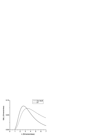
Figure 2: Comparison of our result for $G(\mathbf{0},L)$ (full line) with the result of Shimada and YamakawaShimada and Yamakava (1984) (dashed line).

a form that is in agreement with the results of Shimada and Yamkawa Shimada and Yamakava (1984).  Note that the persistence length of the chain, $l_{p}=\beta\kappa$. We give a compartive plot of the our function and their function $G_{SY}(\mathbf{0,}L)$ ($=896.32e^{-\frac{14.054l_{p}}{L}+0.246L/l_{p}}(l_{p}/L)^{5}$) in Fig. 2. It is clear that there is fair agreement between the two. The value of $L$ at which the maximum occurs is $L=2.63l_{p}$ in our $G(\mathbf{0,}L)$, while it occurs at $L=3.37l_{p}$ for the results of Shimada and Yamakawa Shimada and Yamakava (1984).

It is interesting to ask how the $L^{-5}$ term  in Eq. (79) comes about.   The Dirac delta function $\delta(\mathbf{R)}$ contributes  $L^{-3}$.  $G(\mathbf{0},L)$ would have the ratio of the partition function for the loop conformation to that of the rod, and this contributes a factor of $\left(\beta\kappa/L\right)^{1/2}$.  Further, the fact that the potential energy depends on $\kappa/L$ term causes three factors of $\left(\beta\kappa/L\right)^{1/2}$ (from the three components of $\mathbf{R}$ contained in the probability density at $R_{i}=0,$ with $i=x,y$ or $z$ and comes from the fact that the larger the value of $L$, the broader the distribution of the $R_{i}$).  These multiply together give the factor $\beta^{2}\kappa^{2}/L^{5}$ in Eq. (79).

VI The time for loop formation

We now evaluate the average loop formation time using the approach outlined in Section II.  The quantity $v_{eq}$ is

$$v_{eq}=\left\langle\mathcal{S}(\mathbf{R})\right\rangle$$ (80)

with $\left\langle S(\mathbf{R})\right\rangle$ defined by

$$\left\langle\mathcal{S}(\mathbf{R}))\right\rangle=\frac{1}{Z}\int d\mathbf{\Psi}\int d\mathbf{p_{\mathbf{\Psi}}}\exp(-\beta H[\mathbf{\Psi},\mathbf{p_{\mathbf{\Psi}}}])\mathcal{S}(\mathbf{R}).$$ (81)

Following our discussion in previous Section, we approximate it as

$$\left\langle\mathcal{S}(\mathbf{R})\right\rangle\cong\frac{1}{Z_{R}}\int d\mathbf{\Psi}_{L}\int d\mathbf{p_{\mathbf{\Psi}_{L}}}\exp(-\beta H_{L}[\mathbf{\Psi},\mathbf{p_{\mathbf{\Psi}_{L}}}])\mathcal{S}(\mathbf{R})$$ (82)

It can be easily evaluated, following the methods of Appendix B.  The result is

$$\left\langle\mathcal{S}(\mathbf{R})\right\rangle=16\sqrt{\frac{2\left|\mathbf{T}_{L}^{\phi}\right|}{3\left|\mathbf{T}_{R}^{\phi}\right|}}\frac{e^{-\frac{4L^{2}\pi^{2}\beta\kappa}{3L^{3}+8\pi^{2}\beta\eta^{2}\kappa}}\pi^{3}\beta^{2}\kappa^{2}}{\sqrt{L}\sqrt{L^{3}-4\pi^{2}\beta\eta^{2}\kappa}\sqrt{L^{3}+8\pi^{2}\beta\eta^{2}\kappa}\sqrt{3L^{3}+8\pi^{2}\beta\eta^{2}\kappa}}.$$ (83)

VI.1 The sink-sink correlation function

The essential step in finding the average time of loop formation is to calculate the sink-sink correlation function, Eq. (12). The sink-sink correlation function can be written in terms of  $\mathbf{\Psi}$:

$$\begin{array}[]{c}\mathcal{D}(t)=\int d\mathbf{\Psi}\int d\mathbf{\Psi}^{\prime}\mathcal{S}(\mathbf{R}^{\prime})G_{0}(\mathbf{\Psi}^{\prime},\mathbf{\Psi};t)\mathcal{S}(\mathbf{R})P_{eq}(\mathbf{\Psi}).\end{array}$$ (84)

$G_{0}(\mathbf{\Psi}^{\prime},\mathbf{\Psi};t)$ is the propagator expressed in terms of $\mathbf{\Psi}$ and obeys the condition $G_{0}(\mathbf{\Psi}^{\prime},\mathbf{\Psi};t)\mathcal{S}(\mathbf{R})\rightarrow\delta(\mathbf{\Psi^{\prime}}-\mathbf{\Psi}))$ as $t\rightarrow 0$. The $P_{eq}(\mathbf{\Psi})$ in the above is given by

$$P_{eq}(\mathbf{\Psi})=\frac{1}{Z}\int d\mathbf{\Psi}\int d\mathbf{p_{\mathbf{\Psi}}}\exp(-\beta H[\mathbf{\Psi},\mathbf{p_{\mathbf{\Psi}}}]).$$ (85)

In the spirit of our previous discussions, we approximate $P_{eq}(\mathbf{\Psi})$ near the loop configuration as

$$P_{eq}(\mathbf{\Psi})\cong\frac{1}{Z_{R}}\int d\mathbf{p_{\mathbf{\Psi}_{L}}}\exp(-\beta H_{L}[\mathbf{\Psi},\mathbf{p_{\mathbf{\Psi}_{L}}}]).$$

The sink-sink correlation function may be written as

$$\mathcal{D}(t)=\left\langle\mathcal{S}(\mathbf{R})\right\rangle\mathcal{C}(t),$$ (86)

where

$$\mathcal{C}(t)=\frac{1}{\left\langle S(\mathbf{R})\right\rangle}\int d\mathbf{\Psi}\int d\mathbf{\Psi}^{\prime}\mathcal{S}(\mathbf{R}^{\prime})G_{0}(\mathbf{\Psi}^{\prime},\mathbf{\Psi};t)\mathcal{S}(\mathbf{R})P_{eq}(\mathbf{\Psi}).$$ (87)

$\mathcal{C}(t)$  can now be approximated as

$$\mathcal{C}(t)\cong\mathcal{C}_{a}(t)=\frac{\int d\mathbf{\Psi}_{L}\int d\mathbf{\Psi}_{L}^{\prime}S(\mathbf{R}^{\prime})G_{0}(\mathbf{\Psi}_{L}^{\prime},\mathbf{\Psi}_{L};t)S(\mathbf{R})\exp\left(-\beta\frac{\kappa}{2L}\mathbf{\Psi}_{L}^{{\dagger}}\mathcal{V}_{L}\mathbf{\Psi}_{L}\right)}{\int d\mathbf{\Psi}_{L}\mathcal{S}(\mathbf{R})\exp\left(-\beta\frac{\kappa}{2L}\mathbf{\Psi}_{L}^{{\dagger}}\mathcal{V}_{L}\mathbf{\Psi}_{L}\right)}.$$ (88)

Note that we use the subscript $``a"$ to denote the approximate value of $\mathcal{C}(t)$. The above integral may be re-expressed in terms of the normal modes $\mathbf{Y}$ as

$$\mathcal{C}_{a}(t)\mathbf{=}\frac{\int d\mathbf{Y}^{\prime}\int d\mathbf{Y}\mathcal{S}(\mathbf{R}^{\prime})G_{0}(\mathbf{Y}^{\prime},\mathbf{Y};t)\mathcal{S}(\mathbf{R})\exp\left(-\beta\frac{\kappa}{2L}\mathbf{Y}^{{\dagger}}\mathcal{K}\mathbf{Y}\right)}{\int d\mathbf{Y}\mathcal{S}(\mathbf{R})\exp\left(-\beta\frac{\kappa}{2L}\mathbf{Y}^{{\dagger}}\mathcal{K}\mathbf{Y}\right)}.$$

$G_{0}(\mathbf{Y}^{\prime},\mathbf{Y};t)$ is the propagator expressed in  terms of the normal modes $\mathbf{Y}$.  The Jacobians associated with the transformation in the numerator and denominator cancel out (Note that $\int d\mathbf{Y}^{\prime}G_{0}(\mathbf{Y}^{\prime},\mathbf{Y};t)=1$).  With the above form the sink function, $\mathcal{C}_{a}(t)$ can be evaluated to obtain (see appendix C)

$$\mathcal{C}_{a}(t)=\mathcal{C}_{x}(t)\mathcal{C}_{y}(t)\mathcal{C}_{z}(t)$$ (89)

with

$$\mathcal{C}_{x}(t)=\frac{e^{\frac{1}{2}L^{2}\beta\kappa\left(\frac{1}{S_{x}(0)L^{3}+\beta\eta^{2}\kappa}-\frac{2}{\left(S_{x}(0)+S_{x}(\overline{t})\right)L^{3}+\beta\eta^{2}\kappa}\right)}\sqrt{\beta}\sqrt{\kappa}\sqrt{S_{x}(0)L^{3}+\beta\eta^{2}\kappa}}{\sqrt{2\pi}\sqrt{\left(S_{x}(0)L^{3}+\beta\eta^{2}\kappa\right){}^{2}-L^{6}S_{x}(\overline{t}){}^{2}}},$$ (90)

$$\mathcal{C}_{y}(t)=\frac{\sqrt{\beta}\sqrt{\kappa}\sqrt{S_{y}(0)L^{3}+\beta\eta^{2}\kappa}}{2\sqrt{2}\pi^{3/2}\sqrt{\left(S_{y}(0)L^{3}+\beta\eta^{2}\kappa\right){}^{2}-L^{6}S_{y}(\overline{t}){}^{2}}}$$ (91)

and

$$\mathcal{C}_{z}(t)=\frac{\sqrt{\beta}\sqrt{\kappa}\sqrt{S_{z}(0)L^{3}+\beta\eta^{2}\kappa}}{\sqrt{2}\pi^{5/2}\sqrt{\left(S_{z}(0)L^{3}+\beta\eta^{2}\kappa\right){}^{2}-L^{6}S_{z}(\overline{t}){}^{2}}}.$$ (92)

On using these,

$$\mathcal{C}_{a}(t)=\sqrt{\frac{3\left|\mathbf{T}_{R}^{\phi}\right|}{2\left|\mathbf{T}_{L}^{\phi}\right|\kappa\beta\pi^{15}}}e^{\frac{1}{2}L^{2}\beta\kappa\left(\frac{1}{S_{x}(0)L^{3}+\beta\eta^{2}\kappa}-\frac{2}{\left(S_{x}(0)+S_{x}(\overline{t})\right)L^{3}+\beta\eta^{2}\kappa}+\frac{8\pi^{2}}{3L^{3}+8\pi^{2}\beta\eta^{2}\kappa}\right)}\frac{\sqrt{L}}{128}$$ (93)

$$\frac{\sqrt{\left(L^{3}-2\pi^{2}\beta\eta^{2}\kappa\right)\left(L^{3}+8\pi^{2}\beta\eta^{2}\kappa\right)\left(3L^{3}+8\pi^{2}\beta\eta^{2}\kappa\right)}\sqrt{S_{x}(0)L^{3}+\beta\eta^{2}\kappa}\sqrt{S_{y}(0)L^{3}+\beta\eta^{2}\kappa}\sqrt{2S_{z}(0)L^{3}+2\beta\eta^{2}\kappa}}{\sqrt{\left(S_{x}(0)L^{3}+\beta\eta^{2}\kappa\right){}^{2}-L^{6}S_{x}(\overline{t}){}^{2}}\sqrt{\left(S_{y}(0)L^{3}+\beta\eta^{2}\kappa\right){}^{2}-L^{6}S_{y}(\overline{t}){}^{2}}\sqrt{\left(S_{z}(0)L^{3}+\beta\eta^{2}\kappa\right){}^{2}-L^{6}S_{z}(t){}^{2}}}$$

In the above

$$\begin{array}[]{c}S_{x}(\overline{t})=\sum\limits_{n=1}^{\mathcal{N}}\frac{f_{n}^{2}}{k_{nx}}e^{-\overline{t}k_{nx}}{\mathrm{;}}S_{y}(\overline{t})=\sum\limits_{n=2}^{\mathcal{N}}\frac{g_{n}^{2}}{k_{ny}}e^{-\overline{t}k_{ny}}{\mathrm{;}}S_{z}(\overline{t})=\sum\limits_{n\neq 2}^{\mathcal{N}}\frac{h_{n}^{2}}{k_{nz}}e^{-\overline{t}k_{nz}}.\end{array}$$ (94)

with $\overline{t}=t/\tau_{0}$. $S_{x}(0)$, $S_{y}(0)$ and $S_{z}(0)$ can be evaluated exactly (see Appendix D). Using their values given by equations (135), (137) and (139).  Defining

$$f(\overline{t})=S_{x}(\overline{t})/S_{x}(0),g(\overline{t})=S_{y}(\overline{t})/S_{y}(0);\mbox{and }h(\overline{t})=S_{z}(\overline{t})/S_{z}(0).$$ (95)

we get  

$$C_{a}(t) = \left(\frac{2\beta\kappa}{\pi}\right)^{3/2}e^{\frac{1}{2}L^{2}\beta\kappa\left(\frac{8\pi^{2}}{3\ L^{3}+8\pi^{2}\beta\eta^{2}\kappa}-\frac{16\pi^{2}}{3f(\overline{t})L^{3}+3L^{3}+8\ \pi^{2}\beta\eta^{2}\kappa}\right)}$$

$$\frac{\sqrt{L^{3}-4\ \pi^{2}\beta\eta^{2}\kappa}\sqrt{L^{3}+8\pi^{2}\beta\eta^{2}\ \kappa}\sqrt{3L^{3}+8\pi^{2}\beta\eta^{2}\kappa}}{\ \sqrt{\left(3L^{3}+8\pi^{2}\beta\eta^{2}\kappa\right)^{2}-9L^{6}f(\overline{t})^{2}}\ \sqrt{\left(L^{3}+8\pi^{2}\beta\eta^{2}\kappa\right)^{2}-L^{6}g(\overline{t})^{2}}\ \sqrt{L^{6}\ h(\overline{t})^{2}-\left(L^{3}-4\pi^{2}\beta\eta^{2}\kappa\right)^{2}}}$$

The values of $f_{n}/k_{xn}^{2},g_{n}/k_{yn}^{2}$ and $h_{n}/k_{zn}^{2}$ are given in Table 1.  Use of equations (83) and (VI.1) in Eq. (86) leads to an approximation for $\mathcal{D}(t)$ which we denote by $\mathcal{D}_{a}(t)$.

$$\mathcal{D}_{a}(t)=\left\langle S(\mathbf{R})\right\rangle\mathcal{C}_{a}(t).$$ (97)

Since the eigenvalue $k_{2z}$ is negative (see Table 1), the term $g(t)$ has a term that diverges exponentially as $t\rightarrow\infty$, making $\mathcal{C}_{z}(\infty)=0$.  Hence $\mathcal{D}_{a}(\infty)$ is zero. This is due to the instability along $R_{z}$, which causes the correlation function to vanish at long times. Hence, $\mathcal{D}_{a}(t)$ given by Eq. (97) is a good approximation to $\mathcal{D}(t)$ at short times.  For long times $\mathcal{D}(t)$ will approach $v_{eq}^{2}$.   Hence $\mathcal{D}(t)\cong\mathcal{D}_{a}(t)$ is a valid approximation only at short times. For for long times, $\mathcal{D}(t)$ should be equal to $v_{eq}^{2}$. Hence, it follows that the actual correlation function may be approximated as $\mathcal{D}(t)\cong\mathcal{D}_{a}(t)+v_{eq}^{2}$. Using this in Eq. (11) one gets

$$\tau=\frac{1}{v_{eq}^{2}}\int\limits_{0}^{\infty}\mathcal{D}_{a}(t)dt.$$ (98)

We note that $\beta\kappa=l_{p}$ is the persistence length of the polymer and that $\frac{\rho(\beta\kappa)^{4}\gamma}{\kappa}$ has dimensions of time, and use these as units for length and time.  Then, the expression for $\tau$ becomes

$$\tau=\sqrt{\frac{3\left|\mathbf{T}_{R}^{\phi}\right|}{64\left|\mathbf{T}_{L}^{\phi}\right|\pi^{9}}}L^{9/2}W(L)$$ (99)

with

$$W(L) = \int_{0}^{\infty}dte^{\frac{24L^{5}\pi^{2}\ f(t)}{\left(3L^{3}+8\pi^{2}\eta^{2}\right)\left(3f(t)L^{3}+3L^{3}+8\pi^{2}\eta^{2}\right)}}\left(1-\frac{f(t)^{2}}{\left(1+8\pi^{2}\eta^{2}/3L^{3}\right)^{2}}\right)^{-1/2}$$

$$\left(1-\frac{\ g(t)^{2}}{\left(1+8\pi^{2}\eta^{2}/L^{3}\right)^{2}}\right)^{-1/2}\left(\frac{h(t)^{2}}{\left(1-4\pi^{2}\eta^{2}/L^{3}\right)^{2}}-1\right)^{-1/2}.$$

The functions $f(t),$ $g(t)$ and $h(t)$, on evaluation are found to be given by

$$f(t)=0.995873e^{-298.541t}+0.00408587e^{-7126.56t}.$$ (101)

$$g(t) = 0.921041e^{-1413.12t}+0.0625692e^{-24548.8t}+0.0105256e^{-134918.t}$$ (102)

$$+0.00312111e^{-436308.t}+0.00124791e^{-1.06959\times 10^{6}t}.$$

$$h(t) = 1.02629e^{1241.14t}-0.0197683e^{-28705.1t}-0.00396455e^{-152588.t}$$ (103)

$$-0.00130213e^{-474114.t}.$$

Terms that make no significant contribution to $f(t)$, $g(t)$ and $h(t)$, as their exponents are large and the coefficients small have been neglected in the above. Using Eq. (99), we have calculated the average time of loop formation $\tau$ as a function of the length $L$, and the results are given in figures 3 and 4. The results are dependent on the sink width $\eta$.  The full lines in these figures give exact values of $\tau$ for various values of sink size $\eta.$ The values of $\tau$ for each value of $\eta$ were fitted with an equation of the form $A\exp(E_{a}/L)L^{n}$ and the values of $E_{a}$ and $n$, as well as the value of the length at which $\tau$ is a minimum ($L_{m}$) is given in Table 2.  The curves that result from the fitting are shown as dotted lines in the figures.  It is seen that the functional form $\tau=A\exp(E_{a}/L)L^{n}$ reproduces the data well, with the exponent in the prefactor $n$ being dependent on $\eta$ and varying from $4.5$ to $6$.  For small $\eta,$ $n$ is close to $6$.  Further, the loop formation time $\tau$ becomes longer and longer as $\eta$ is made smaller. In fact, as may be seen by from Eq. (99), the time diverges like $1/\eta$ as $\eta\rightarrow 0$ (see Eq. (105)). This is not surprising, because as $\eta\rightarrow 0$, the diffusional search for loop formation is for a smaller and smaller volume in space. In fact, on looking at Eq. (99) and remembering that $\eta$ actually serves the purpose of a small length cut off, one would have expected the dependence to be approximately

$$\tau=A\exp(E_{a}/L)L^{9/2}.$$ (104)

However, there are two reasons that lead to the observed dependence on $\eta$. (1) The exponential term in Eq. (VI.1) is dependent on $t$ and makes the $L$ dependence change from the simple form of Eq. (104) and (2) the $L$ dependence of the terms inside the square roots in Eq. (VI.1).  From the functional forms of $f(t),$ $g(t)$ and $h(t),$ it is clear that due to the presence of $h(t),$ the integrand decreases rather rapidly. For $t\sim 1/\omega_{h},$where $\omega_{h}=1241.4$ (see Eq. 101) $\left(\frac{h(t)^{2}}{\left(1-4\pi^{2}\eta^{2}/L^{3}\right)^{2}}-1\right)^{-1/2}\cong h(t)^{-1}=$ $(1/1.02629)e^{-\omega_{h}t}$ .   On this time scale ($t\sim 1/\omega_{h}$), one can approximate $\left(1-\frac{\ g(t)^{2}}{\left(1+8\pi^{2}\eta^{2}/L^{3}\right)^{2}}\right)^{-1/2}\cong 1$ and $\left(1-\frac{f(t)^{2}}{\left(1+8\pi^{2}\eta^{2}/3L^{3}\right)^{2}}\right)^{-1/2}$ $\cong\left(3L^{3}/16\pi^{2}\eta^{2}\right)^{1/2}.$  Hence for small values of $\eta$, the integral may be evaluated approximately to get

$$\tau_{close}(L)=\frac{3}{32\omega_{h}\eta}\sqrt{\frac{\left|\mathbf{T}_{R}^{\phi}\right|}{\left|\mathbf{T}_{L}^{\phi}\right|\pi^{11}}}L^{6}e^{\frac{4\pi^{2}\ }{3L}}.$$ (105)

Thus for small $\eta$ the loop formation time behaves like $\sim L^{6}e^{\frac{4\pi^{2}\ }{3L}}$ as seen in the Table 2. For not so small values of $\eta,$ one expects $\left(1-\frac{f(t)^{2}}{\left(1+8\pi^{2}\eta^{2}/3L^{3}\right)^{2}}\right)^{-1/2}$ $\cong 1$ and $\left(1-\frac{\ g(t)^{2}}{\left(1+8\pi^{2}\eta^{2}/L^{3}\right)^{2}}\right)^{-1/2}\cong 1$.  This leads to $n\sim 9/2$.

Physically, the above results are easy to understand.  The rate of the loop formation may be written as $\simeq\mathcal{P}(R_{x}\lesssim\eta,R_{y}\lesssim\eta,R_{z}\lesssim\eta)\times$ frequency factor $\times Z_{L}/Z_{R}$.   In this, $\mathcal{P}(\mathbf{R})$ is the probablity distribution function for the end-to-end vector.  For a semi-flexible chain, the frequency factor $\sim L^{-4}.$  In the limit $\eta\rightarrow 0,$ $\mathcal{P}(R_{x}\lesssim\eta,R_{y}\lesssim\eta,R_{z}\lesssim\eta)\sim$ $(\beta\kappa/L)^{3/2}$ as seen earlier and $Z_{L}/Z_{R}\sim(\beta\kappa/L)^{1/2}$.  Therefore, the preexponential factor of the rate has $(\beta\kappa)^{2}/L^{6}$ dependence.  On the other hand, as one increases the value of $\eta$, for sufficiently large $\eta$, $\mathcal{P}(R_{x}\lesssim\eta,R_{y}\lesssim\eta,R_{z}\lesssim\eta)=1$, leading to rate of the form $(\beta\kappa)^{1/2}/L^{9/2}$ref .

VI.2
Numerical Results

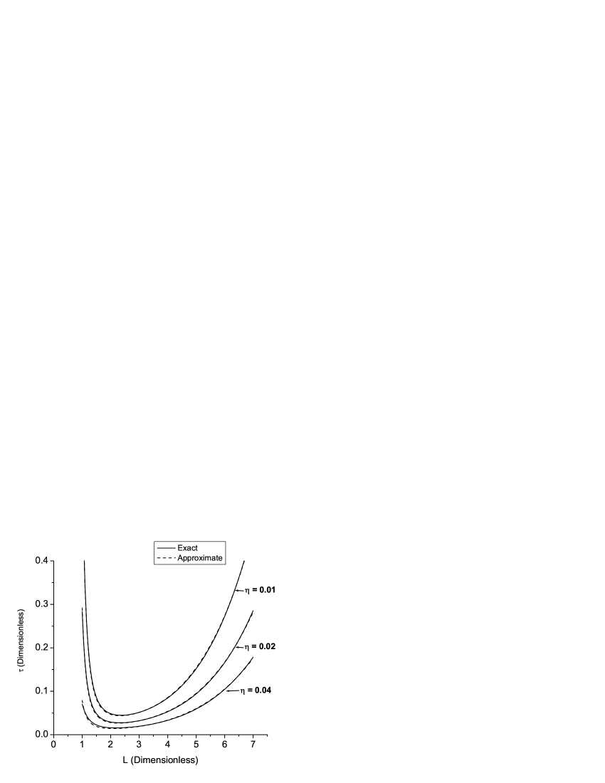
Figure 3: The time of loop formation, $\tau$ as a function of $L$, for different values of the width $\eta$. Units are chosen such that both $\tau$ and $L$ dimensionless. The full curves are the computed results. They are well represented by the functional form $AL^{n}\exp(E_{a}/L)$ as may be seen from the figure, where we have represented them by dotted lines. The parameters that result from fitting are given in Table 2.

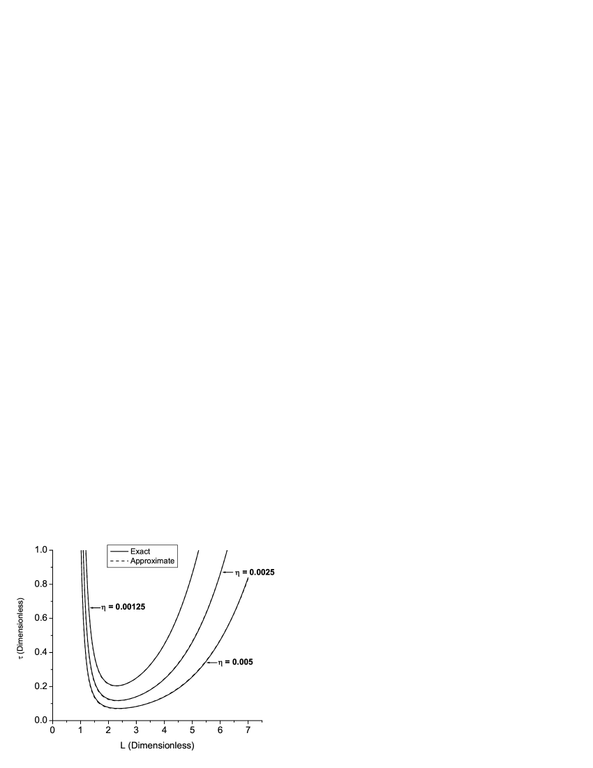
Figure 4: The closing time $\tau$ as a function of $L$, for different values of the width $\eta$. Units are adopted such that all these are dimensionless. The full curves are the computed results. They are well represented by the functional form $AL^{n}\exp(E_{a}/L)$ as may be seen from the figure, where we have represented them by dotted lines. The parameters that result from fitting are given in Table 2.

$\eta$	$A\times 10^{6}$	$E_{a}$	$n$	$L_{m}$
0.04	2.800	10.247	4.920	2.19
0.02	1.823	11.982	5.261	2.32
0.01	1.627	12.890	5.51	2.37
0.005	1.740	13.421	5.74	2.37
0.0025	2.268	13.64	5.90	2.33
0.00125	3.670	13.65	5.99	2.28

Table 2: Fitted Parameters: Values of $A$, $E_{a}$ and $n$ and $L_{m}$ (the dimensionless length at which $\tau$ is a minimum).

We now consider loop formation of double stranded DNA, which has a persistence length of $50$ nm. The sink function, defined by Eq. (13) and (14) has a width equal to $\eta$ which may be taken as $\ 2-3$ Å.   Then the dimensionless $\eta$ would have a value of roughly $1/200$ and this would correspond to the lowest curve in Fig. 4, with $n=5.9$.  On the other hand for a more flexible chain, with persistence length equal to $2.5$ nm, and with a value of $\eta$ equal to $1$ Å, one would have dimensionless $\eta=1/25,$ and this would correspond to the lowest curve in Fig. 3 with $n=4.9$.   The value of $L_{m}$ at which the minmum time is required for loop formation, does not depend strongly on the value of $\eta$.  Thus it is found to be in the range $2.2$ to $2.4$ times the persistence length of the chain (see Table 2).

The dynamics of loop formation in semiflexible polymers was analyzed by Dua and Cherayil, who found $\tau\sim L^{n},$ with $n$ $\sim 2.2-2.4$, with $n$ approaching $2$ in the flexible limit.  This is obviously valid in the longer chain limit.  On the other hand, Jun et al Jun and Bechhoefer (2003); Jun et al. (2003) have studied the region where the length of the chain is a few times the persistence length.  The assumed the two ends of the chain to execute random walk with a constant diffusion coefficient, and found that there is a length ($L_{m}$) at which $\tau$ is a minimum.   Their analysis used accurate results for $G(\mathbf{0},L)$ and lead to somewhat larger value for $L_{m}$ ($3-4$). On the other hand, we have studied the dynamics in detail, using a multimode approach.  We get expressions for $G(\mathbf{0},L)$ and $\tau$ which have extrema at lower values of $L$, this being a result of the use of approximate expression for the bending energy.

VII Summary and Conclusions

In this work, we have presented a detailed multi-dimensional analysis of the loop formation dynamics of semiflexible chains. The reverse process, the opening of the loop was studied in a previous work Santo and Sebastian (2006), where we developed an approximate model for a semiflexible chain in the rod limit. In this model, the conformations of the polymer are mapped onto the paths of a random walker on the surface of a unit sphere. The bending energy of the chain was expanded about a minimum energy path. This model was shown to be a good approximation for the polymer in the rod limit and provided an easy way to describe the dynamics. Use of this model led to opening rates of a semiflexible polymer loop formed by a weak bond between the ends. in Ref. Santo and Sebastian (2006), we calculated the opening rates for a Morse type interaction between the ends of the polymer as a function of the contour length of the chain. In this paper, we analyzed the loop formation dynamics using this model and thus, presented a rather complete theory of dynamics of formation of semiflexible polymer loops.

The dynamics was described using the formalism by Wilemski and Fixman, which describe the intra-chain reactions of polymers as a diffusion-controlled reaction. In this formalism, the reaction process is described using a sink function. For an arbitrary sink function, exact results are not available and hence, WF introduced an approximation called “closure approximation”. In this procedure, the closing time can be expressed in terms of a sink-sink correlation function. To calculate this sink-sink correlation function and thereby the closing time, one needs to know the Green’s function of the chain and the equilibrium distribution. We calculated the Green’s function of the chain through a normal mode analysis near the loop geometry. This normal mode analysis could be performed independently of the rigidity ($\kappa$) and contour length ($L$) of the polymer, leading to a set of eigenvalues that are universal. An approximate equilibrium distribution for the polymer near the ring configuration was given. As the sink function vanishes for large values of the end-to-end distance $R$, sink-sink correlation function has contributions mostly from the dynamics of the polymer near the ring configurations. We calculated this approximate sink-sink correlation function for a Gaussian sink through a transformation of variables into normal coordinates.

We then obtained loop formation time (in dimensionless units), $\tau$ for different contour lengths of the chain. We found that $\tau\sim L^{9/2}W(L)$, where $W(L)$ is an integral that could be performed numerically. Numerical calculations lead to the result that $\tau=AL^{n}\exp(E_{a}/L)$, with $n$ varying between $9/2$ and $6$. $\tau$ was found to have a minimum at $L_{min}=2.2$ to $2.4$ which is to be compared with the values $3.4$ obtained by Jun et. al. Jun et al. (2003) by a simple one dimensional analysis and the value $2.85$ of Chen et. al. Chen et al. (2004) found through simulations Chen et al. (2004).

ACKNOWLEDGEMENTS

K. P. Santo thanks Council of Scientific and Industrial Research (CSIR), India for financial support and Cochin University of Science and Technology (CUSAT), Kochi, India for providing computer facilities during the preparation of the manuscript.  The work of KLS is supported by the J.C. Bose Fellowship of the Department of Science and Technology, Govt. of India.

Appendix A The kinetic energy of the ring and the rod

The kinetic energy Eq. (38) of the polymer may be evaluated using Eq. (22). We take $\mathbf{r}_{cm}=0$, so that the ring is described in the center of mass frame and the translational degrees of freedom are eliminated.

A.1 Matrix elements for the Loop

The kinetic energy matrix elements of the loop are given below.

A.1.1 Odd $\phi$ Modes

For odd $\delta\phi_{n}$ modes one has

$$(\mathbf{T}_{L}^{\phi o})_{mn}=t_{n}\delta_{mn}-16t_{n}t_{m},$$ (106)

where

$$t_{n}=\frac{4+n^{2}}{2(-4+n^{2})^{2}\pi^{2}}.$$ (107)

A.1.2 Even $\phi$ Modes

For even $\delta\phi_{n}$, one has

$$(\mathbf{T}_{L}^{\phi e})_{mn}=t_{n}\delta_{mn}$$ (108)

with $n,m\neq 2$. For $m,n=2$ one gets

$$(\mathbf{T}_{L}^{\phi e})_{22}=\frac{-3+4\pi^{2}}{192\pi^{2}}$$ (109)

and

$$(\mathbf{T}_{L}^{\phi e})_{2n}=-\frac{4+n^{2}}{2(-4+n^{2})^{2}\pi^{2}}=(\mathbf{T}_{L}^{\phi e})_{n2}$$ (110)

A.1.3 Odd $\theta$ Modes

The kinetic energy matrix corresponding to the even $\theta$ modes have the following form. For $n,m\neq 0$

$$(\mathbf{T}_{L}^{\theta o})_{nm}=q_{n}\delta_{mn}$$ (111)

where

$$q_{n}=\frac{1}{2n^{2}\pi^{2}}.$$ (112)

For the zeroth mode

$$(\mathbf{T}_{L}^{\theta o})_{00}=\frac{1}{12}$$ (113)

and

$$(\mathbf{T}_{L}^{\theta o})_{0n}=-\frac{1}{n^{2}\pi^{2}}=(\mathbf{T}_{L}^{\theta})_{n0}.$$ (114)

A.1.4 Even $\theta$ Modes

The kinetic energy matrix corresponding to the odd $\theta$ modes have the following form

$$(\mathbf{T}_{L}^{\theta e})_{nm}=q_{n}\delta_{mn}-d_{n}d_{m},$$ (115)

where

$$q_{n}=\frac{1}{2n^{2}\pi^{2}}$$ (116)

and

$$d_{n}=-\frac{2}{n^{2}\pi^{2}}.$$ (117)

A.2 For the Rod

In the case of a rod, the matrix elements are identical for $\phi$ and $\theta$ modes.  They are given by

$$(\mathbf{T}_{R}^{\phi o})_{mn}=(\mathbf{T}_{R}^{\theta o})_{mn}=t_{n}^{\prime}\delta_{mn}-16t_{n}^{\prime}t_{m}^{\prime},$$ (118)

where

$$t_{n}^{\prime}=\frac{1}{2n^{2}\pi^{2}}.$$ (119)

For modes with even $n$ one has

$$(\mathbf{T}_{R}^{\phi e})_{mn}=(\mathbf{T}_{R}^{\theta e})_{mn}=t_{n}^{\prime}\delta_{mn}$$ (120)

with $n,m\neq 0$. In this case, the zeroth mode is couples to the other modes. Thus one gets

$$(\mathbf{T}_{R}^{\phi e})_{00}=(\mathbf{T}_{R}^{\theta e})_{00}=\frac{1}{12}$$ (121)

and

$$(\mathbf{T}_{R}^{\phi e})_{0n}=(\mathbf{T}_{R}^{\theta e})_{0n}=\frac{1}{n^{2}\pi^{2}}=(\mathbf{T}_{R}^{\phi e})_{n0}.$$ (122)

Appendix B The evaluation of $G(\mathbf{0,}L)$

We now give details of the evaluation of $G(\mathbf{0,}L)$ . We perform the integral in Eq. (77) and substitute the value of $Z_{R}$ from Eq. (72) to get

$$G(\mathbf{0,}L\mathbf{)} = \frac{8\pi^{2}}{Z_{R}}\int d\mathbf{p}_{\mathbf{\Psi}_{L}}\int d\mathbf{\Psi}_{L}\exp(-\beta H_{L})\delta(\mathbf{R)}\delta(\delta\phi_{0})\delta(\delta\theta_{2c})\delta(\delta\theta_{2s}).$$ (123)

$$= \pi 2^{3-4\mathcal{N}}\left(\frac{\kappa\beta\pi}{3}\right)^{2\mathcal{N}-1}\sqrt{\frac{\left|\mathbf{T}_{L}^{\phi}\right|}{\left|\mathbf{T}_{R}^{\phi}\right|}}G^{\phi o}G^{\phi e}G^{\theta o}G^{\theta e},$$ (124)

where $G^{\phi o}G^{\phi e}G^{\theta o}G^{\theta e}$ are defined and calculated in the following.  $G^{\phi o}$ is the contribution from the odd $\phi$ modes to $G(\mathbf{0,}L\mathbf{)}$ and is defined by

$$G^{\theta o}=\prod\limits_{n,odd}\int d\delta\theta_{n}\exp\left(-\frac{\beta\kappa\pi^{2}}{4L}(n^{2}-4)\delta\theta_{n}^{2}\right)\delta(\delta\theta_{2s}).$$ (125)

We put $\delta(\delta\theta_{2s})=(1/2\pi)\int dp\exp(ip\delta\theta_{2s})=(1/2\pi)\int dp\exp(2pi\sum\limits_{n,odd}a_{n}\delta\theta_{n})$.  With this, integrals over $\delta\theta_{n}$ with $n=3,5,..$ are evaluated and then the one over $p$, after which one can easily evaluate the integral over $\delta\theta_{1}.$ The result is

$$G^{\theta o}=\sqrt{\frac{\pi}{3}}\left(\frac{\pi\kappa\beta}{L}\right)^{(1-\mathcal{N})/2}\frac{2}{\sqrt{\Gamma(\mathcal{N}-1/2)\Gamma(\mathcal{N}+3/2)}}$$ (126)

$\Gamma$ is the Gamma function. $\ G^{\theta e}$ is the contribution from the even $\theta$ modes to $G(\mathbf{0,}L\mathbf{)}$ and is defined by

$$G^{\theta e}=\prod\limits_{n,even}\int d\delta\theta_{n}\exp\left(-\frac{\beta\kappa\pi^{2}}{4L}(n^{2}-4)\delta\theta_{n}^{2}\right)\delta(\delta\theta_{2})\delta(L\delta\theta_{0})$$

The $\delta(L\delta\theta_{0})$ comes as the $\delta(R_{z})$ part of $\delta(\mathbf{R})$ in Eq. (123).  The integrals are easy and the result is

$$G^{\theta e}=\sqrt{\frac{2\pi\kappa\beta}{L^{3}}}\left(\frac{\pi\kappa\beta}{L}\right)^{(1-\mathcal{N})/2}\frac{1}{\sqrt{\Gamma(\mathcal{N}-1)\Gamma(\mathcal{N}+1)}}$$ (127)

$G^{\phi e}$ is the contribution from the even $\phi$ modes to $G(\mathbf{0,}L\mathbf{)}$ and is defined by

$$G^{\phi e}=\prod\limits_{n,even}\int d\delta\phi_{n}\exp\left(-\frac{\beta\kappa\pi^{2}}{4L}n^{2}\delta\phi_{n}^{2}\right)\delta(\delta\phi_{0})\delta(L\delta\phi_{2}/2)$$ (128)

The $\delta(\delta\phi_{0})$ comes as a result of removing the rotational mode $\delta\phi_{0}.$ (123).  The integrals are easy and the result is

$$G^{\phi e}=\frac{2}{L}\left(\frac{\pi\kappa\beta}{L}\right)^{(1-\mathcal{N}/2)}\frac{1}{\Gamma(\mathcal{N})}$$ (129)

$G^{\phi o}$ is the contribution from the odd $\phi$ modes to $G(\mathbf{0,}L\mathbf{)}$ and is defined by

$$G^{\phi o}=\prod\limits_{n,odd}\int d\delta\phi_{n}^{\prime}\exp\left(-\frac{\beta\kappa\pi^{2}}{4L}n^{2}(\delta\phi_{n}^{{}^{\prime}})^{2}\right)\delta\left(L\sum_{n,odd}a_{n}\left(\delta\phi_{n}^{\prime}+\frac{8}{n^{2}\pi}\right)\right)$$

On evaluation, we get

$$G^{\phi o}=\frac{2}{\sqrt{3\beta\kappa L}}\left(\frac{\pi\kappa\beta}{L}\right)^{(1-\mathcal{N})/2}\frac{1}{\Gamma(\mathcal{N}+1/2)}\exp(-\frac{4\pi^{2}\kappa\beta}{3L})$$ (130)

The equations (126), (127), (130) and (129) above combined together with (123)  and with $\mathcal{N}\rightarrow\infty$ taken, gives

$$G(\mathbf{0,}L\mathbf{)=}\frac{16\sqrt{2}\pi^{3}\beta^{2}\kappa^{2}}{3L^{5}}\sqrt{\frac{\left|\mathbf{T}_{L}^{\phi}\right|}{\left|\mathbf{T}_{R}^{\phi}\right|}}\exp\left(-\frac{4\pi^{2}\beta\kappa}{3L}\right)$$ (131)

The ratio $\sqrt{\frac{\left|\mathbf{T}_{L}^{\phi}\right|}{\left|\mathbf{T}_{R}^{\phi}\right|}}$ can be evaluated using MATHEMATICA, taking each to be $1000\times 1000$ matrices.  It evaluates to

$$\sqrt{\frac{\left|\mathbf{T}_{L}^{\phi}\right|}{\left|\mathbf{T}_{R}^{\phi}\right|}}=6.5083.$$ (132)

Appendix C The evaluation of $\left\langle S(\mathbf{R})\right\rangle$ and $\mathcal{C}(t).$

The evaluation of $\left\langle S(\mathbf{R})\right\rangle$ and $\mathcal{C}(t)$ are similar to the evaluation of $G(\mathbf{0},L)$ carried out in Appendix B.  The result for $\left\langle S(\mathbf{R})\right\rangle$ is

$$\left\langle S(\mathbf{R})\right\rangle=\sqrt{\frac{2\left|\mathbf{T}_{L}^{\phi}\right|}{3\left|\mathbf{T}_{R}^{\phi}\right|}}\frac{16e^{-\frac{4L^{2}\pi^{2}\beta\kappa}{3L^{3}+8\pi^{2}\beta\eta^{2}\kappa}}\pi^{3}\beta^{2}\kappa^{2}}{\sqrt{L}\sqrt{L^{3}-4\pi^{2}\beta\eta^{2}\kappa}\sqrt{L^{3}+8\pi^{2}\beta\eta^{2}\kappa}\sqrt{3L^{3}+8\pi^{2}\beta\eta^{2}\kappa}}$$ (133)

$\mathcal{C}(t)$ may be written as a product of three terms, as already seen in Eq. (89).  We give expressions for them the following.

$$\mathcal{C}_{x}(t)=\frac{\left(\prod\limits_{n=1}^{\mathcal{N}}\int dY_{n}^{\prime}\int dY_{n}G(Y_{n}^{\prime}\mathbf{,}t|Y_{n},0\mathbf{)}\exp\left(-\frac{\beta\kappa}{2L}k_{nx}Y_{n}^{2}\right)\right)S_{x}\left(L\sum\limits_{l=1}^{\mathcal{N}}f_{l}Y_{l}^{\prime}+L\right)S_{x}\left(L\sum\limits_{m=1}^{\mathcal{N}}f_{m}Y_{m}+L)\right)}{\left(\prod\limits_{n=1}^{\mathcal{N}}\int dY_{n}\exp\left(-\frac{\beta\kappa}{2L}k_{nx}Y_{n}^{2}\right)\right)S_{x}\left(L\sum\limits_{m=1}^{\mathcal{N}}f_{m}Y_{m}+L)\right)}.$$

$\mathcal{C}_{y}(t)$ and $\mathcal{C}_{z}(t)$ are defined by

$$\mathcal{C}_{y}(t)=\frac{\left(\prod\limits_{n=\mathcal{N}+1}^{2\mathcal{N}}\int dY_{n}^{\prime}\int dY_{n}G(Y_{n}^{\prime}\mathbf{,}t|Y_{n},0\mathbf{)}\exp\left(-\frac{\beta\kappa}{2L}k_{nx}Y_{n}^{2}\right)\right)S_{y}\left(L\sum\limits_{l=\mathcal{N}+1}^{2\mathcal{N}}g_{l}Y_{l}^{\prime}\right)S_{y}\left(L\sum\limits_{m=\mathcal{N}+1}^{2\mathcal{N}}g_{m}Y_{m}\right)}{\left(\prod\limits_{n=\mathcal{N}+1}^{2\mathcal{N}}\int dY_{n}\exp\left(-\frac{\beta\kappa}{2L}k_{nx}Y_{n}^{2}\right)\right)S_{y}\left(L\sum\limits_{m=\mathcal{N}+1}^{2\mathcal{N}}g_{m}Y_{m}\right)}.$$

$$\mathcal{C}_{z}(t)=\frac{\left(\prod\limits_{n=2\mathcal{N}+1}^{3\mathcal{N}}\int dY_{n}^{\prime}\int dY_{n}G(Y_{n}^{\prime}\mathbf{,}t|Y_{n},0\mathbf{)}\exp\left(-\frac{\beta\kappa}{2L}k_{nx}Y_{n}^{2}\right)\right)S_{z}\left(L\sum\limits_{l=2\mathcal{N}+1}^{3\mathcal{N}}h_{l}Y_{l}^{\prime}\right)S_{z}\left(L\sum\limits_{m=2\mathcal{N}+1}^{3\mathcal{N}}g_{m}Y_{m}\right)}{\left(\prod\limits_{n=2\mathcal{N}+1}^{3\mathcal{N}}\int dY_{n}\exp\left(-\frac{\beta\kappa}{2L}k_{nx}Y_{n}^{2}\right)\right)S_{z}\left(L\sum\limits_{m=2\mathcal{N}+1}^{3\mathcal{N}}h_{m}Y_{m}\right)}.$$

On performing the integrations, one gets $\mathcal{C}_{x}(t),\mathcal{C}_{y}(t)$ and $\mathcal{C}_{z}(t)$ given in equations (90) to (92).

Appendix D The evaluation of $S_{x}(0),$ $S_{y}(0)$ and $S_{z}(0)$

The value of $S_{x}(0)$ can be found as follows. Defining the vectors $\mathbf{f}=(f_{1},f_{2},....f_{\mathcal{N}})$ and $\mathbf{a}=(a_{1},a_{3},....a_{{2\mathcal{N}}-1})$, $S_{x}(0)$ is given by

$$S_{x}(0)=\sum\limits_{n=1}^{\mathcal{N}}\frac{f_{n}^{2}}{k_{nx}}$$ (134)

Using Equations (46) and (54), we get

$$\begin{array}[]{c}S_{x}(0)=\mathbf{a.(T}_{L}^{\phi o})^{-1/2}\mathbf{U}^{\phi o}\left(\mathbf{U}^{\phi o\dagger}\mathbf{(T}_{L}^{\phi o})^{-1/2}\mathbf{V}^{\phi o}\mathbf{(T}_{L}^{\phi o})^{-1/2}\mathbf{U}^{\phi o}\right)^{-1}\mathbf{U}^{\phi o\dagger}\mathbf{(T}_{L}^{\phi o})^{-1/2}.\mathbf{a}^{\dagger}\\ =\mathbf{a.}\left(\mathbf{V}_{L}^{\phi o}\right)^{-1}.\mathbf{a}^{\dagger}\\ =\sum\limits_{n=odd}^{\infty}\frac{2a_{n}^{2}}{n^{2}\pi^{2}}=\frac{3}{8\pi^{2}}.\end{array}$$ (135)

Similarly, using Eq. (46) and (56) gives

$$S_{y}(0) = \sum\limits_{n}\frac{g_{n}^{2}}{k_{ny}}=$$ (137)

$$\frac{1}{4}\left[\mathbf{(T}_{L}^{\phi e})^{-1/2}\mathbf{U}^{\phi e}\left(\mathbf{U}^{\phi e\dagger}\mathbf{(T}_{L}^{\phi e})^{-1/2}\mathbf{V}_{L}^{\phi e}\mathbf{(T}_{L}^{\phi e})^{-1/2}\mathbf{U}^{\phi e}\right)^{-1}\mathbf{U}^{\phi e\dagger}\mathbf{(T}_{L}^{\phi o})^{-1/2}\right]_{22}$$

$$= \frac{1}{4}(\mathbf{V}_{L}^{\phi e})_{22}^{-1}=\frac{1}{8\pi^{2}},$$ (138)

and in a similar fashion

$$S_{z}(0)=\frac{1}{4}(\mathbf{V}_{1}^{\theta e})_{00}^{-1}=\frac{-1}{4\pi^{2}}.$$ (139)

References

• Santo and Sebastian (2006) K. P. Santo and K. L. Sebastian, Phys. Rev. E 73, 031293 (2006).
• Rippe (2001) K. Rippe, Trends in Biochemical Science 26, 733 (2001).
• Rippe et al. (1995) K. Rippe, P. H. V. Hippel, and J. Langowski, Trends in Biochemical Science 20, 500 (1995).
• Jun and Bechhoefer (2003) S. Jun and J. Bechhoefer, Physics in Canada 59, 85 (2003).
• Bonnet et al. (1998) G. Bonnet, O. Krichevsky, and A. Libchaber, Proc. Natl. Acad. Sci. USA 95, 8602 (1998).
• Wallace et al. (2001) M. I. Wallace, L. Ying, S. Balasubramanian, and D. Klenerman, Proc. Natl. Acad. Sci. USA 98, 5584 (2001).
• Goddard et al. (2000) N. L. Goddard, G. Bonnet, O. Krichevisky, and A. Libchaber, Phys. Rev. Lett. 85, 2400 (2000).
• Ansari et al. (2001) A. Ansari, S. V. Kuznetsov, and Y. Shen, Proc. Natl. Accad. Sci. USA 98, 7771 (2001).
• Shen et al. (2001) Y. Shen, S. V. Kuznetsov, and A. Ansari, J. Phys. Chem. B 105, 12202 (2001).
• Lapidus et al. (2002) L. J. Lapidus, P. J. Steinbach, W. A. Eaton, A. Szabo, and J. Hofrichter, J. Phys. Chem. B 106, 11628 (2002).
• Hagen et al. (2002) S. J. Hagen, J. Hofrichter, A. Szabo, and W. A. Eaton, Proc. Natl. Accad. Sci. USA 106, 11628 (2002).
• Lapidus et al. (2000) L. J. Lapidus, W. A. Eaton, and J. Hofrichter, Proc. Natl. Accad. Sci. USA 97, 7220 (2000).
• Lapidus et al. (2001) L. J. Lapidus, W. A. Eaton, and J. Hofrichter, Phys. Rev. Lett. 87, 258101 (2001).
• Wilemski and Fixman (1974) G. Wilemski and M. Fixman, J. Chem. Phys. 60, 878 (1974).
• Doi (1975) M. Doi, Chem. Phys. 9, 455 (1975).
• Szabo et al. (1980) A. Szabo, K. Schulten, and Z. Schulten, J. Chem. Phys. 72, 4350 (1980).
• Srinivas et al. (2002) G. Srinivas, K. L. Sebastian, and B. Bagchi, J. Chem. Phys. 116, 7276 (2002).
• Pastor et al. (1996) R. W. Pastor, R. Zwanzig, and A. Szabo, J. Chem. Phys 105, 3878 (1996).
• Wilhelm and Frey (1996) J. Wilhelm and E. Frey, Phys. Rev. Lett. 77, 2561 (1996).
• Chirikjian and Wang (2000) G. S. Chirikjian and Y. Wang, Phys.Rev. E 62, 880 (2000).
• Winkler et al. (1994) R. G. Winkler, P. Reineker, and L. Harnau, J. Chem. Phys. 101, 8119 (1994).
• Freed (1971) K. F. Freed, J. Chem. Phys. 54, 1453 (1971).
• Harris and Hearst (1966) R. A. Harris and J. E. Hearst, J. Chem. Phys. 44, 2595 (1966).
• Saito et al. (1967) N. Saito, K. Takahashi, and Y. Yunoki, J. Phy. Soc. Jpn. 22, 219 (1967).
• Yamakawa and Stockmayer (1972) H. Yamakawa and W. Stockmayer, J. Chem. Phys. 57, 2843 (1972).
• Shimada and Yamakava (1984) J. Shimada and H. Yamakava, Macromolecules 17, 689 (1984).
• Dua and Cherayil (2002) A. Dua and B. Cherayil, J. Chem. Phys. 117, 7765 (2002).
• Jun et al. (2003) S. Jun, J. Bechhoefer, and B. Y. Ha, Europhys. Lett. 64, 420 (2003).
• Chen et al. (2004) J. Z. Y. Chen, H. K. Tsao, and Y.-J.Sheng, Europhys. Lett. 65, 407 (2004).
• Ranjith et al. (2005) P. Ranjith, P. B. S. Kumar, and G. I. Menon, Physical Review Letters 94, 138102 (2005).
• Kulic and Schiessel (2003) I. M. Kulic and H. Schiessel, Biophys. J 84, 3197 (2003).
• Bicout and Szabo (1997) D. J. Bicout and A. Szabo, J. Chem. Phys. 106, 10292 (1997).
• Sebastian (1992) K. L. Sebastian, Phys. Rev. A 46, R1732 (1992).
• Debnath et al. (2006) A. Debnath, R. Chakrabarti, and K. L. Sebastian, Journal of Chemical Physics 124, 204111 (2006).
• Gardiner (1983) C. Gardiner, Handbook of Stochastic Methods (Springer, 1983).
• Risken (1989) H. Risken, The Fokker-Plank Equation (Springer, 1989).
• (37) We thank a referee for insightful remarks, which lead to these conclusions.