High Energy Behavior of a Six-Point $R$-Current Correlator in ${\cal N}=4$ Supersymmetric Yang-Mills Theory

Abstract:

We study the high energy limit of a six-point $R$-current correlator in ${\cal N}=4$ supersymmetric Yang-Mills theory for finite $N_{c}$. We make use of the framework of perturbative resummation of large logarithms of the energy. More specifically, we apply the (extended) generalized leading logarithmic approximation. We find that the same conformally invariant two-to-four gluon vertex occurs as in non-supersymmetric Yang-Mills theory. As a new feature we find a direct coupling of the four-gluon $t$-channel state to the $R$-current impact factor.

1 Introduction

The high energy limit of nonabelian gauge theories, in particular of QCD, has been extensively studied in a variety of perturbative and nonperturbative approaches. In the groundbreaking work of [1, 2] the perturbative resummation of leading logarithms of the center-of-mass energy $\sqrt{s}$ was performed. The resulting leading logarithmic approximation (LLA) is encoded in the celebrated BFKL equation. It collects all perturbative terms of the order $(\alpha_{s}\log s)^{m}$ in which the smallness of the strong coupling constant $\alpha_{s}$ is compensated by large logarithms of the energy. For the scattering amplitude of $2\to 2$ scattering processes, this leading logarithmic approximation corresponds to resumming diagrams in which two interacting reggeized gluons are exchanged in the $t$-channel. This bound state of two gluons, the Pomeron, can hence be represented diagrammatically by a gluon ladder.

Based on Gribov’s work on the Reggeon calculus [3] it was immediately clear that, once such moving Regge singularities exist, the high energy behavior of nonabelian gauge theories can be formulated in terms of an effective 2+1 dimensional field theory, called Reggeon field theory. It lives in the two transverse dimensions of the scattering process, and rapidity can be understood as a timelike parameter. Steps towards explicitly formulating this effective high energy description include the generalization of the BFKL approximation to the evolution of $n$-gluon states, known as the BKP equations [4, 5], and a further generalization which encompasses number-changing processes during the $t$-channel evolution. The latter is known as the (extended) generalized leading logarithmic approximation, (E)GLLA, and will be described in some detail later in this paper. It has been used to derive a $2\to 4$ gluon vertex that contains the triple Pomeron vertex [6, 7, 8], as well as a higher order $2\to 6$ gluon vertex function [9]. A systematic approach of deriving, for nonabelian gauge theories, the elements of Reggeon field theory, is the effective action developed in [10, 11], see [12]. Other approaches to the problem of understanding the high energy limit of QCD include the Wilson line operator expansion [13]-[16], the dipole picture of high energy scattering [17]-[20], and the color glass condensate approach, see for example [21]. In the limit $N_{c}\to\infty$ the latter three approaches as well as the EGLLA all give rise to the same non-linear evolution equation, known as the BK equation [13, 22, 23]. All approaches mentioned here are of perturbative nature. A nonperturbative derivation of a Reggeon field theory from QCD still appears prohibitively difficult.

Among the most remarkable features of Reggeon field theory for QCD are the conformal invariance in the two-dimensional transverse coordinate space [24, 25, 26], and the integrability in the large-$N_{c}$ limit [27, 28, 29]. Both properties, so far, have been established only for the leading order of the resummation in the LLA and (E)GLLA. A full understanding of the fate of these symmetries in next-to-leading order is still missing.

With the advent of the AdS/CFT correspondence, which relates the maximally supersymmetric nonabelian gauge theory in four dimensions, that is ${\cal N}=4$ super Yang-Mills theory (SYM) with gauge group $\text{SU}(N_{c})$, to type IIB superstring theory on a five-dimensional AdS space [30, 31, 32], the natural question appears whether Reggeon field theory has a dual analog on the string (or supergravity) side. As a first step, one identifies scattering amplitudes or correlators which are defined on both sides of the correspondence: in QCD, a clean environment for studying the dynamics at high energies has been found in $\gamma^{*}\gamma^{*}$ scattering, i. e. in the four-point correlators of electromagnetic currents. In ${\cal N}=4$ SYM, it has been suggested [33] to consider, as a substitute for the $\mbox{U}(1)$ current of electromagnetism, the $R$-currents which result from the global $\text{SU}_{R}(4)$ $R$-symmetry. One is thus led to investigate, in suitable high energy limits, correlators of $R$-currents, both for ${\cal N}=4$ SYM and for the dual string theory.

On the gauge theory side, existing QCD calculations provide a natural starting point for a systematic investigation of this correspondence. It is, however, clear that certain differences exist between (non-supersymmetric) QCD and ${\cal N}=4$ SYM, and one has to study their consequences. For the high energy behavior of current correlators, it is the impact factors which are sensitive to supersymmetry: in QCD, the fermions (quarks) belong to the fundamental representation of the gauge group, whereas in ${\cal N}=4$ SYM all particles (gluons, Weyl fermions and scalars) are in the adjoint representation of the gauge group. On the other hand, since in quantum field theory the high energy behavior is dominated by the exchange of particles with the highest spin – that is the gluons in both theories – the leading logarithmic approximation in ${\cal N}=4$ SYM should be quite similar to QCD.

As the very first step, the elastic scattering of two $R$-currents in ${\cal N}=4$ SYM has been studied in [34]. Apart from the new impact factors, it has been verified that the high energy behavior is dominated by the familiar BFKL Pomeron. Turning to elements of Reggeon field theory beyond the BFKL two-gluon ladders, the effect of supersymmetry is expected to be more severe. As a theoretical environment for extracting the triple Pomeron vertex calculations on the QCD side have made use of six-point functions. This motivates, for the extension to ${\cal N}=4$ SYM, to investigate six-point correlators of $R$-currents. It is the purpose of the present paper to study the high energy behavior of such $R$-current correlators in the extended generalized leading logarithmic approximation. As a result we will find that ${\cal N}=4$ SYM provides a new element in Reggeon field theory which is not present in non-supersymmetric QCD. On the other hand, the triple Pomeron vertex remains the same as in QCD. We emphasize that throughout this paper we keep $N_{c}$ finite, and we only briefly comment on the large-$N_{c}$ limit at the end.

Parallel to this investigation of the gauge theory side, it is interesting to study the $R$-current correlators in the same kinematic limit also on the string side. Here, in the simplest approximation, one considers the zero slope limit and arrives at Witten diagrams with graviton exchanges. For the elastic scattering this has been done in [35], while for the problem of the six-point function work along these lines is in progress.

Our paper is organized as follows. In section 2 we define the triple-Regge limit of six-point correlators, first for virtual photons in QCD, then for $R$-currents in ${\cal N}=4$ SYM theory. In section 3 we consider the $R$-current impact factors, consisting of the sum of a Weyl fermion loop and a scalar loop in the adjoint representation with $n$ gluons attached. We derive the relation of these impact factors to the corresponding impact factors consisting of quark loops in the fundamental representation, and present them explicitly for up to four gluons. We put special emphasis on the reggeization of the impact factors. Further in that section we point out that the Odderon decouples from impact factors containing particles in the adjoint representation. In section 4 we write down the integral equations which sum all diagrams contributing to the (extended) generalized leading logarithmic approximation. In section 5 we study these integral equations, tracing in particular the consequences of the new impact factors obtained before. In section 6 we finally present our result for the six-point correlator which differs from the result in QCD. Section 7 contains our conclusions and an outlook. Appendix A deals with some $\text{su}(N_{c})$ color identities. In two further appendices we consider higher $n$-gluon amplitudes and their reggeization in ${\cal N}=4$ SYM: In appendix B we generalize our findings for the four-gluon amplitude to five gluons. In appendix C, finally, we make some steps towards a calculation of the six-gluon amplitude. These first steps already allow us to draw some conclusions about the 2-to-6 gluon transition function in ${\cal N}=4$ SYM. Some results presented in this paper have been published in a letter [36].

2 Six-point correlation functions at high energies

In this section we define the high energy limit of six-point functions in ${\cal N}=4$ SYM. As is well known, the high energy behavior of scattering amplitudes in the Regge limit is determined by the exchange of particles with the highest spin which, in the case of ${\cal N}=4$ SYM, are the gauge bosons with spin 1. Studies of the high energy behavior of Yang-Mills theories in the leading logarithmic approximation show that, apart from the impact factors, the high energy behavior is entirely determined by the gauge bosons. This implies that, in this approximation, in a supersymmetric extension of non-supersymmetric $\text{SU}(N_{c})$ gauge theory, e. g. in ${\cal N}=4$ SYM with the same gauge group, the difference between the supersymmetric and the non-supersymmetric theory resides in the impact factors. Specifically, in supersymmetric theories the fermion fields are in the adjoint representation, and in addition to the impact factors consisting of closed fermion loops we have also those composed of scalar particles. Apart from the impact factors, the interactions of the exchanged gluons are the same as in the non-supersymmetric case.

2.1 Six-point amplitudes in QCD

In QCD, scattering amplitudes with more than $4$ external particles arise naturally in the context of deep inelastic scattering on a weakly bound nucleus. A simple example is deep inelastic scattering (DIS) on a nucleus consisting of two weakly bound nucleons (that is a deuteron), see figure 1.

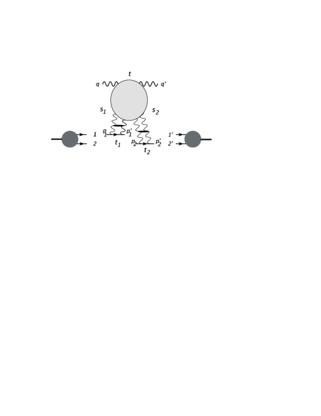
Figure 1: Scattering of a virtual photon on a weakly bound nucleus

The total cross section of this scattering process is obtained from the elastic scattering amplitude, $T_{\gamma^{*}(pn)\to\gamma^{*}(pn)}$, via the optical theorem,

$$\sigma^{\rm tot}_{\gamma^{*}(pn)\to\gamma^{*}(pn)}=\frac{1}{S}\,{\rm Im}\,T_{\gamma^{*}(pn)\to\gamma^{*}(pn)}\,,$$ (1)

where $S=(q+p_{1}+p_{2})^{2}$ denotes the total energy of the scattering process. In order to obtain an entirely perturbative environment, we can think of replacing the two nucleons by virtual photons. As a result, we are led to six-point correlators of (off-shell) electromagnetic currents, $T_{\gamma^{*}\gamma^{*}\gamma^{*}\to\gamma^{*}\gamma^{*}\gamma^{*}}$, where the coupling between the external electromagnetic currents and the exchanged gluons is mediated by three photon impact factors.

Let us start with the amplitude $T_{\gamma^{*}(pn)\to\gamma^{*}(pn)}$. The kinematics is illustrated in figure 1: the amplitude depends upon three energy variables, $s_{1}=(q+p_{1})^{2}$, $s_{2}=(q^{\prime}+p^{\prime}_{2})^{2}$, and $M^{2}=(q+p_{1}-p^{\prime}_{1})^{2}$. In the high energy limit that we are interested in, $s_{1}\simeq s_{2}\simeq s$ and all these variables are of the same order as $S=(q+p_{1}+p_{2})^{2}\simeq 2s$. All these energies are assumed to be much larger than the momentum transfer variables $t=(q-q^{\prime})^{2}$, $t_{1}=(p_{1}-p^{\prime}_{1})^{2}$, and $t_{2}=(p_{2}-p^{\prime}_{2})^{2}$ and the virtuality of the photon, $Q^{2}=-q^{2}$,

$$s_{1},s_{2}\gg M^{2}\gg Q^{2},-t_{1},-t_{2},-t\,.$$ (2)

We will distinguish between $s_{1}$ and $s_{2}$, but at the end we set $s_{1}=s_{2}=s$ and $t=0$. Throughout this paper we use Sudakov variables with the lightlike reference vectors $q_{A}$ and $p_{B}$, such that $s=2q_{A}\cdot q_{B}$, $S=4q_{A}\cdot p_{B}=2s$, $q=q_{A}-xp_{B}$ with $x=Q^{2}/(2q_{A}\cdot p_{B})$ and

$$x_{P}=\frac{M^{2}+Q^{2}-t_{1}}{s}\simeq\frac{M^{2}}{s}\ll 1\,.$$ (3)

Neglecting the nucleon masses we have

$$p_{1}=p_{2}=p_{B}\,,\>\>\>\>\>\>p^{\prime}_{1}=p_{B}(1-x_{P})+p_{1\perp}\,,\>\>\>\>\>\>p^{\prime}_{2}=p_{B}(1+x_{P})+p_{2\perp}\,.$$ (4)

Internal momenta are then written as

$$k_{i}=\alpha_{i}q_{A}+\beta_{i}p_{B}+k_{i\,\perp}$$ (5)

with $k^{2}_{i\,\perp}=-{\bf k}_{i}^{2}$. The fact that the two nucleons are in a weakly coupled bound state implies that we will allow the two nucleons to have small losses of longitudinal and transverse momenta, i. e. we will integrate over $x_{P}$ and $p_{1\perp}=-p_{2\perp}=k_{\perp}$. The integration over $x_{P}$ is equivalent to the integration over the mass squared $M^{2}$, and the latter will be kept much smaller than $s$.

A convenient way of computing the elastic scattering amplitude $T_{\gamma^{*}(pn)\to\gamma^{*}(pn)}$ in the high energy limit is to use dispersion relations and Regge theory, for a review of these techniques see [37]. For our case the scattering amplitude can be written in the form

$$\begin{split}T_{3\to 3}&(s_{1},s_{2},M^{2};t_{1},t_{2},t)\\ &=\int\frac{dj_{1}dj_{2}dj}{(2\pi i)^{3}}\,s_{1}^{j_{1}}\xi(j_{1}){s_{2}}^{j_{2}}\xi(j_{2})(M^{2})^{j-j_{1}-j_{2}}\xi(j,j_{1},j_{2})F(j_{1},j_{2},j;t_{1},t_{2},t)\end{split}$$ (6)

with the signature factors $\xi(j)=-\pi\frac{e^{-i\pi j}+1}{\sin\pi j}$, $\xi(j,j_{1},j_{2})=-\pi\frac{e^{-i\pi(j-j_{1}-j_{2})}+1}{\sin\pi(j-j_{1}-j_{2})}$. Given the representation (6), there is an easy way of computing this amplitude. Namely, we take the triple discontinuity in $s_{1}$, $s_{2}$, and $M^{2}$,

$${\rm disc}_{s_{1}}\,{\rm disc}_{s_{2}}\,{\rm disc}_{M^{2}}T_{3\to 3}=\pi^{3}\int\frac{dj_{1}dj_{2}dj}{(2\pi i)^{3}}s_{1}^{j_{1}}{s_{2}}^{j_{2}}(M^{2})^{j-j_{1}-j_{2}}F(j_{1},j_{2},j;t_{1},t_{2},t)\,,$$ (7)

and see that the partial wave $F(j_{1},j_{2},j;t_{1},t_{2},t)$ which in our kinematic region is real-valued (i. e. has no internal phases) can be computed from the triple Mellin transform of the (real-valued) triple energy discontinuity. Using unitarity, this triple energy discontinuity is easily obtained from high energy production processes.

To obtain the cross section (1) for deep inelastic scattering on the deuteron from eq. (6) it is needed to take the imaginary part, i. e. the discontinuity in $M^{2}$, to set $s_{1}=s_{2}=s$ and $t=0$ (which implies $p_{1\perp}=-p_{2\perp}=k_{\perp}$), and to integrate over the phase space of the two nucleons, i. e. over $x_{P}=M^{2}/s$ and ${k_{\perp}}$,

$$\begin{split}\sigma^{\text{tot}}_{\gamma^{*}(pn)\to}&{}_{\gamma^{*}(pn)}(s)=\frac{1}{2s}\int_{x}^{1}{dx_{P}}\int\!\!\frac{d^{2}{\bf k}}{2(2\pi)^{3}}\,\text{disc}_{M^{2}}T_{3\to 3}(s,s,M^{2}=x_{P}s;-{\bf k}^{2},-{\bf k}^{2},0)\\ =&{}\,\frac{1}{2}\int\frac{dj_{1}dj_{2}dj}{(2\pi i)^{3}}\,s^{j-1}\xi(j_{1})\xi(j_{2})\,\frac{1}{j-j_{1}-j_{2}+1}\int\!\!\frac{d^{2}{\bf k}}{2(2\pi)^{3}}\,F(j_{1},j_{2},j;-{\bf k}^{2},-{\bf k}^{2},0)\,,\end{split}$$ (8)

where due to the nucleon form factors the integration over ${\bf k}^{2}=-t_{1}=-t_{2}$ remains restricted to a small range.

For the discussion of this paper, however, we focus on the correlator of six currents, $T_{3\to 3}(s_{1},s_{2},M^{2};t_{1},t_{2},t)$, and the integrations over $x_{P}$ and ${\bf k}$ will not be considered. In the following it will be convenient to introduce instead of the angular momenta $j$, $j_{1}$, $j_{2}$ the variables $\omega=j-1$, $\omega_{1}=j_{1}-1$, $\omega_{2}=j_{2}-1$, and we will write $F(\omega_{1},\omega_{2},\omega;t_{1},t_{2},t)$ instead of $F(j_{1},j_{2},j;t_{1},t_{2},t)$.

In order to form, in the leading logarithmic approximation, color singlet $t$-channel states which couple at the top to the virtual photon and at the bottom to two photons, one is led to QCD diagrams with four $t$-channel gluons at the lower end and two, three, or four gluons at the upper end. A few examples of such diagrams are shown in figure 2. Wavy $t$-channel gluon lines stand for reggeized gluon propagators, and horizontal lines between the $t$-channel gluons denote on-shell $s$-channel gluons (that is real gluon production in the interaction kernel).

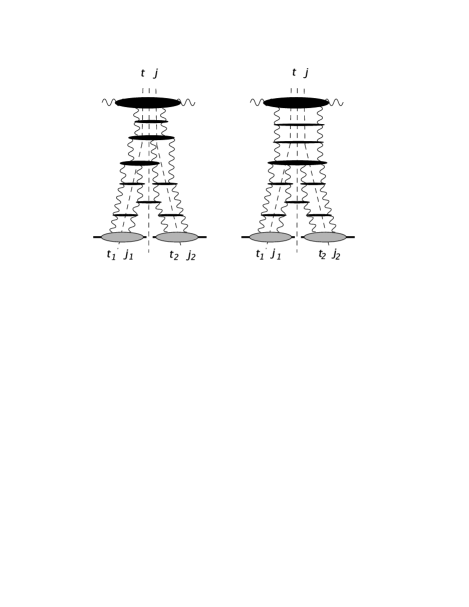
Figure 2: A few contributions to the triple energy discontinuity in eq. (6)

For the computation of the triple energy discontinuity we proceed in the same way as for the LO BFKL ladders. We use multiparticle amplitudes in the multi-Regge kinematics: $T_{2\to n}$ and, more generally, $T_{n\to m}$, where all incoming and outgoing particles are separated by large rapidity gaps. These diagrams represent, for the six-point amplitude in the triple Regge limit, the (generalized) leading logarithmic approximation: for each gluon loop we have a logarithm of a large energy variable.

As to the general structure of the diagrams, at the lower end we start from 4 reggeized gluons (two color singlets) which couple to the two impact factors at the bottom. At the upper end, given by the upper photon impact factor, we end with a $t$-channel state consisting of two, three, or four gluons. We thus encounter $t$-channel states with $2$, $3$, or $4$ gluons: their propagation is described by the BFKL equation for the case of two gluons, and by the BKP equations in the case of three and four gluons. When moving from the bottom to the top, the number of $t$-channel gluons never increases. Transitions between the different states are described by kernels $K_{2\to 3}$ and $K_{2\to 4}$ which we describe in section 4.3 below. There are three different $t$-channels ($t$, $t_{1}$, $t_{2}$), and each of them has its own angular momentum $\omega$, $\omega_{1}$, $\omega_{2}$, respectively. As seen from figure 2, there is always a ‘lowest’ interaction, which we call ‘branching vertex’, below which the diagrams split into the $t_{1}$ and $t_{2}$ channels. It is therefore convenient to split the diagrams of figure 2 into three pieces: below the branching vertex we have two disconnected BFKL Pomerons, $D_{2}$, depending on $\omega_{1}$ and $\omega_{2}$, respectively. At and above the vertex we have an amplitude with four gluons, $D_{4}$, which depends upon $\omega$: it satisfies an integral equation which, for the case of QCD, has been discussed in [8], and has been further studied in [9]. One of the main results of that analysis is the appearance of the Möbius invariant $2\to 4$ gluon vertex. Together with the BFKL kernel it represents one of the fundamental building blocks of QCD Reggeon field theory. The investigation of the analogous amplitude in ${\cal N}=4$ SYM, ${\mathchoice{\hbox{$\displaystyle\mathbb{D}$}}{\hbox{$\textstyle\mathbb{D}$}}{\hbox{$\scriptstyle\mathbb{D}$}}{\hbox{$\scriptscriptstyle\mathbb{D}$}}}_{4}(\omega)$, will be the main goal of the present paper. In particular, we will study the influence of the supersymmetric particle content of the impact factors on the solution of the integral equation for that amplitude.

It is straightforward to generalize this discussion of six-point amplitudes to eight-point, ten-point amplitudes etc. In the same way as the six-point amplitude leads to $4$ gluons in the $t$-channel, the eight-point amplitude contains up to $6$ gluons. As in the previous case, in QCD such amplitudes arise very naturally in the context of the scattering of a photon on nuclei consisting of three or more weakly bound nucleons. From the theoretical point of view, these multiparticle correlators provide a natural environment for color singlet BKP states. When deriving and analyzing these higher order BKP states within QCD, new transition vertices of reggeized gluons appear which are elements of QCD Reggeon field theory. In this paper we restrict ourselves to the six-point amplitude containing four gluons. We will, however, present a few results also on the five- and six-gluon states.

2.2 Six-point correlators of $R$-currents in ${\cal N}=4$ SYM

After this brief review of QCD calculations we now want to turn to analogous scattering amplitudes in ${\cal N}=4$ SYM. In terms of component fields, this theory contains the vector field $A_{\mu}$, 4 chiral spinors $\lambda_{I}$, and 6 real scalars $X_{M}$. They all transform in the adjoint representation of the gauge group $\text{SU}(N_{c})$, and generically we can write the fields as $\Phi=\Phi_{ab}=\Phi^{c}(T^{c})_{ab}$, with the generators of the adjoint representation, $(T^{c})_{ab}=-if_{abc}$. The $f_{abc}$ are the $\mbox{SU}(N_{c})$ structure constants which occur also in the algebra of the generators $t^{a}$ of the fundamental representation, $[t^{a},t^{b}]=if_{abc}t^{c}$. Our convention for the normalization of the $t^{a}$ is such that $\mbox{tr}\,(t^{a}t^{b})=\delta_{ab}/2$. For the generators in the adjoint representation we have $[T^{a},T^{b}]=if_{abc}T^{c}$ and $\mbox{tr}\,(T^{a}T^{b})=N_{c}\delta_{ab}$.

The Lagrangian of ${\cal N}=4$ SYM theory is [38]

$$\begin{split}{\cal L}=\mbox{tr}\,\Big{(}&-\frac{1}{2}F_{\mu\nu}F^{\mu\nu}+D_{\mu}X_{M}D^{\mu}X_{M}+2i\lambda_{I}\sigma^{\mu}D_{\mu}\bar{\lambda}^{I}\\ &-2ig\lambda_{I}[\lambda_{J},X^{IJ}]-2ig\bar{\lambda}^{I}[\bar{\lambda}^{J},X_{IJ}]+\frac{1}{2}g^{2}[X_{M},X_{N}][X_{M},X_{N}]\Big{)}\,.\end{split}$$ (9)

The $X_{M}$ and $X_{IJ}$ are related by the $\text{SU}(4)\cong\text{SO}(6)$ sigma symbols,

$$X_{IJ}=-\frac{1}{2}(\Sigma_{M})_{IJ}X_{M}\,,\qquad\qquad X^{IJ}=\frac{1}{2}(\Sigma^{-1}_{M})^{IJ}X_{M}\,,$$ (10)

with $\mbox{tr}\,(\Sigma_{M}\Sigma_{N}^{-1})=4\delta_{MN}$, which implies that $X_{M}X_{M}=X_{IJ}X^{IJ}$. Capital indices transform under the $R$-symmetry group $\text{SU}(4)$. In particular, $A,B,C,...=1,...,15$ are indices of the adjoint representation, $I,J,K,...=1,...,4$ transform under the fundamental, and $M,N,...=1,...,6$ under the vector representations of the $R$-symmetry. Small indices $a,b,c,...=1,...,N_{c}^{2}-1$ are adjoint representation indices for the gauge group $\text{SU}(N_{c})$. The covariant derivative $D_{\mu}$ and the gauge field strength tensor $F_{\mu\nu}$ are defined in the usual way by (writing $\Phi$ generically for any field in the theory)

$$D_{\mu}\Phi = {}\partial_{\mu}\Phi-ig[A_{\mu},\Phi]\,,$$ (11)

$$F_{\mu\nu} = {}\partial_{\mu}A_{\nu}-\partial_{\nu}A_{\mu}-ig[A_{\mu},A_{\nu}]\,.$$ (12)

The theory enjoys a $\mbox{SU}_{R}(4)$ global symmetry, called $R$-symmetry, which transforms the different supercharges. Under these transformations, the fields $A_{\mu}$, $\lambda_{I}$, $X_{M}$ belong to the scalar, fundamental, and vector representation, respectively. More specifically, the Lagrangian (9) is invariant under the global $R$-symmetry transformation

$$\begin{array}[]{lcl}\delta\lambda^{a\alpha I}&=&{}i\epsilon_{A}\lambda^{a\alpha J}(T^{A})_{JI}\,,\\ \delta\bar{\lambda}^{a\dot{\alpha}I}&=&{}-i\epsilon_{A}(T^{A})_{IJ}\bar{\lambda}^{a\dot{\alpha}J}\,,\\ \delta X^{a}_{M}&=&{}i\epsilon_{A}(T^{A})_{MN}X^{a}_{N}\,,\end{array}$$ (13)

where $\epsilon_{A}$ are small parameters, and $T^{A}$ are the $\mbox{SU}_{R}(4)$ generators in the appropriate representation. The corresponding Noether current is

$$J_{R}^{A\mu}=i\frac{\partial{\cal L}}{\partial(\partial_{\mu}\Phi)}\Delta^{A}\Phi=\mbox{tr}\,\left(-\lambda\sigma^{\mu}T^{A}\bar{\lambda}-iXT^{A}D^{\mu}X\right)\,,$$ (14)

where $\Delta^{A}\Phi$ is obtained from (13) with the definition $\delta\Phi=i\epsilon_{A}\Delta^{A}\Phi$ for an infinitesimal $R$-transformation.

In [33] it has been suggested that in ${\cal N}=4$ SYM this global current can be used as a substitute for the electromagnetic $\mbox{U}(1)$ current in QCD. To be more precise, one should choose an abelian subgroup of the global $\text{SU}_{R}(4)$, for example the one generated by $T^{3}=\mbox{diag}(\frac{1}{2},-\frac{1}{2},0,0)$. The simplest application of this procedure is the supersymmetric analog of elastic $\gamma^{*}\gamma^{*}$ scattering: the elastic scattering of two $R$-currents [34]. In QCD this process, when evaluated at energies much larger than the photon virtualities, provides one of the cleanest environments for studying the BFKL Pomeron. With the conjectured AdS/CFT duality, the correlator of four $R$-currents therefore offers the possibility to study the dual of the BFKL Pomeron on the string theory side.

As a next step along this line, one may address higher correlators, e. g. the six-point function for which the QCD side has been discussed above. Giving labels $A$, $B_{1}$, $B_{2}$ to the three incoming virtual photons (and analogous primed labels to the outgoing ones) in the amplitude $T_{\gamma^{*}\gamma^{*}\gamma^{*}\to\gamma^{*}\gamma^{*}\gamma^{*}}$, one is led to consider an analogous process in ${\cal N}=4$ SYM by defining the momentum space six-point function (see figure 3)

$$i(2\pi)^{4} \delta(q+p_{1}+p_{2}-q^{\prime}-p^{\prime}_{1}-p^{\prime}_{2})\,T_{3\to 3}^{\mu_{A}\mu_{B_{1}}\mu_{B_{2}}\mu_{A^{\prime}}\mu_{B^{\prime}_{1}}\mu_{B^{\prime}_{2}}}$$

$$= \prod_{i=A,...,B^{\prime}_{2}}\int d^{4}x_{i}\,e^{-iq\cdot x_{A}-ip_{1}\cdot x_{B_{1}}-ip_{2}\cdot x_{B_{2}}+iq^{\prime}\cdot x_{A^{\prime}}+ip^{\prime}_{1}\cdot x_{B^{\prime}_{1}}+ip^{\prime}_{2}\cdot x_{B^{\prime}_{2}}}$$

$$\langle J_{R}^{A\mu_{A}}(x_{A})J_{R}^{B_{1}\mu_{B_{1}}}(x_{B_{1}})J_{R}^{B_{2}\mu_{B_{2}}}(x_{B_{2}})J_{R}^{A^{\prime}\mu_{A^{\prime}}}(x_{A^{\prime}})J_{R}^{B^{\prime}_{1}\mu_{B^{\prime}_{1}}}(x_{B^{\prime}_{1}})J_{R}^{B^{\prime}_{2}\mu_{B^{\prime}_{2}}}(x_{B^{\prime}_{2}})\rangle\,.$$ (15)

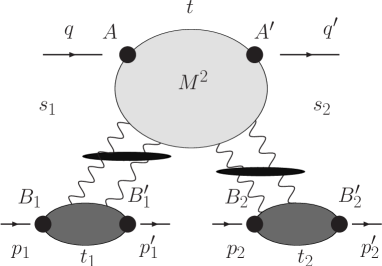
Figure 3: The momentum space six-point function of $3\to 3$ $R$-current scattering.

Following the discussion of the previous subsection, we will be interested in the (generalized) leading logarithmic approximation of the six-point function $T_{3\to 3}$ in the triple Regge limit, where we will make use of the analytic representation (6).

The only places where the supersymmetric content of ${\cal N}=4$ SYM becomes visible in the above expression are the impact factors. Compared to the QCD case, there are two novel features:(i) the (Weyl) fermions are in the adjoint representation, (ii) in addition to the fermion loop, we have the scalars which occur in the adjoint representation as well. In [34] these impact factors have been calculated for the four-point function where two $t$-channel gluons are coupled to the external currents. For the six-point function, new impact factors with three or four $t$-channel gluons appear as well. They have not been calculated yet, and their computation constitutes one of the main goals of this paper.

The structure of these novel impact factors has quite important consequences. In the QCD analysis the integral equations which formally sum all the Reggeon diagrams can partially be solved and simplified. The key ingredients to this are the reggeization of the gluon and the validity of bootstrap equations. The latter ones strongly depend upon the structure of the impact factors which – in QCD with quarks in the fundamental representation – are simple (Dirac) fermion loops. In QCD it has been shown that all contributions with more than two $t$-channel gluons are absorbed into reggeizing pieces, and, at the end, only two-gluon contributions remain. This result is closely connected with the structure of the $2\to 4$ gluon vertex. In the case of ${\cal N}=4$ SYM the fermions are in the adjoint representation, and the impact factors also contain contributions from the scalars: the structure of the impact factors with three or more $t$-channel vector particles is different, and it is a priori not obvious how this affects the solution of the integral equations. We shall investigate this issue in the present paper.

3 Impact factors

3.1 Four-point functions in ${\cal N}=4$ SYM

It will be useful to briefly recapitulate the two-gluon impact factor which was studied in detail in [34], some properties of this impact factor were also discussed in [39, 40]. Its precise definition is given by

$${\mathchoice{\hbox{$\displaystyle\mathbb{D}$}}{\hbox{$\textstyle\mathbb{D}$}}{\hbox{$\scriptstyle\mathbb{D}$}}{\hbox{$\scriptscriptstyle\mathbb{D}$}}}_{(2;0)}^{a_{1}a_{2},\lambda_{A}\lambda_{A^{\prime}}}({\bf k}_{1},{\bf k}_{2})=\,\frac{p_{B}^{\rho_{1}}p_{B}^{\rho_{2}}}{s^{2}}\int_{0}^{\infty}\frac{d\tilde{s}}{2\pi}\,\text{disc}_{\tilde{s}}\,A^{\mu_{A}\mu_{A^{\prime}},\rho_{1}\rho_{2};a_{1}a_{2}}_{R_{A}g_{1}\to R_{A^{\prime}}g_{2}}\epsilon^{\lambda_{A}}_{\mu_{A}}(q)\epsilon^{\lambda_{A^{\prime}}}_{\mu_{A^{\prime}}}(q^{\prime})\,.$$ (16)

Here $A^{\mu_{A}\mu_{A^{\prime}},\rho_{1}\rho_{2};a_{1}a_{2}}_{R_{A}g_{1}\to R_{A^{\prime}}g_{2}}$ is the amplitude for scattering of the $R$-current $A$ with Lorentz index $\mu_{A}$ and a gluon with momentum $-k_{1}$, Lorentz index $\rho_{1}$ and color label $a_{1}$ into the $R$-current $A^{\prime}$ with Lorentz index $\mu_{A^{\prime}}$ and a gluon with momentum $k_{2}$, Lorentz index $\rho_{2}$ and color label $a_{2}$. $\tilde{s}=(q-k_{1})^{2}\simeq q^{2}-{\bf k}_{1}^{2}-s\beta$ is the total center-of-mass energy squared of the $R$-current-gluon system. $\epsilon_{\mu}^{\lambda}(k)$ are the polarization vectors of the $R$-currents with polarizations $\lambda=L,h$ where $L$ denotes longitudinal and $h=1,2$ transverse polarizations.

We begin our discussion with the fermionic part of the $R$-current impact factor which consists of Weyl fermions in the adjoint representation of $\text{SU}(N_{c})$. Compared to Dirac fermions in the fundamental representation (that is the usual QCD case), we have to consider the following changes. Instead of $N_{c}$ fundamental quarks we now have $N_{c}^{2}-1$ adjoint particles, i. e. the color trace $\mbox{tr}\,(t^{a}t^{b})=\delta_{ab}/2$ is replaced by $\mbox{tr}\,(T^{a}T^{b})=N_{c}\delta_{ab}$ where $(T^{a})_{bc}=-if_{abc}$ are the generators in the adjoint representation. Next, we have to consider the $\mbox{U}(1)$ charges $e_{F}$ of the global $\text{SU}_{R}(4)$ symmetry of the Weyl fermions which are the analogs of the electric charges $e_{q}$ in QCD. With our choice of the $\text{U}(1)$ subgroup, $T^{3}={\rm diag}(\frac{1}{2},-\frac{1}{2},0,0)$, we can take care of these charge factors by multiplying the QCD amplitude by

$$R_{F}=\frac{\sum e_{F}^{2}}{\sum e_{q}^{2}}=\frac{1}{2\sum e_{q}^{2}}\,,$$ (17)

since here $\sum e_{F}^{2}=\mbox{tr}\,_{4}(T^{A}T^{A})=\frac{1}{2}$. Furthermore, we identify the left- and right-handed components of a massless Dirac fermion with Weyl fermions in the standard way, and we can conclude that the impact factor with a massless Dirac fermion is twice the corresponding impact factor with a Weyl fermion. Compared to a Dirac fermion in the fundamental representation in QCD, we therefore have for the fermionic contribution in ${\cal N}=4$ SYM the relative weight

$$2N_{c}R\quad\quad\mbox{with}\quad\quad R=\frac{1}{2}R_{F}=\frac{1}{4\sum e_{q}^{2}}\,.$$ (18)

The momentum structure, including the integration over the loop momentum, on the other hand, remains the same in each individual diagram and is not affected by the change of the color representation of the quarks. Finally, we have the scalar contribution for which there is no counterpart in QCD.

In the following we often compare with the QCD case, i. e. with the case of Dirac fermions in the fundamental representation. In order to make a clear distinction between the impact factors (and, later on, also the gluon amplitudes) in the two theories we will denote $n$-gluon impact factors in QCD with fundamental quarks by normal letters, for example $D_{(n;0)}$, while those in ${\cal N}=4$ SYM will be denoted by blackboard-style letters, for example ${\mathchoice{\hbox{$\displaystyle\mathbb{D}$}}{\hbox{$\textstyle\mathbb{D}$}}{\hbox{$\scriptstyle\mathbb{D}$}}{\hbox{$\scriptscriptstyle\mathbb{D}$}}}_{(n;0)}$.

The full ${\cal N}=4$ SYM impact factor ${\mathchoice{\hbox{$\displaystyle\mathbb{D}$}}{\hbox{$\textstyle\mathbb{D}$}}{\hbox{$\scriptstyle\mathbb{D}$}}{\hbox{$\scriptscriptstyle\mathbb{D}$}}}_{(2;0)}({\bf k}_{1},{\bf k}_{2})$ for the scattering of two $R$-currents with two exchanged gluons in the $t$-channel has been computed in [34]. The computation of the fermionic part includes the four diagrams shown in figure 4.

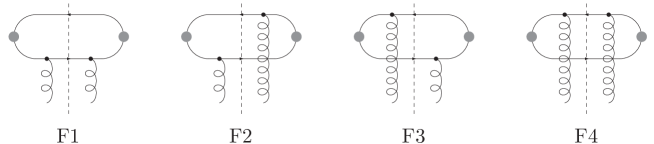
Figure 4: The fermion diagrams for the impact factors.

We consider the discontinuity in $s$ and therefore two propagators are set on-shell. Due to the cut only diagrams in which the gluon lines do not cross have to be included. The external currents are projected onto different polarizations, longitudinal or transverse. For simplicity we give the result of the fermion impact factor, the sum of the four diagrams in figure 4, only for transverse polarization of the $R$-currents:

$${\mathchoice{\hbox{$\displaystyle\mathbb{D}$}}{\hbox{$\textstyle\mathbb{D}$}}{\hbox{$\scriptstyle\mathbb{D}$}}{\hbox{$\scriptscriptstyle\mathbb{D}$}}}_{F,(2;0)}^{a_{1}a_{2},hh^{\prime}}({\bf k}_{1},{\bf k}_{2}) = {}\delta_{a_{1}a_{2}}\,\frac{N_{c}\alpha_{s}}{2}\int_{0}^{1}d\alpha\int\frac{d^{2}{{\bf l}}}{(2\pi)^{2}}$$ (19)

$${}\times\left[-4\alpha(1-\alpha){\mbox{\boldmath$\epsilon$}}^{(h)}\cdot\left(\frac{\mbox{\boldmath$N$}_{1}}{D_{1}}-\frac{\mbox{\boldmath$N$}_{2}}{D_{2}}\right)\left(\frac{\mbox{\boldmath$N$}_{1}^{\prime}}{D_{1}^{\prime}}-\frac{\mbox{\boldmath$N$}_{2}^{\prime}}{D_{2}^{\prime}}\right)\cdot{\mbox{\boldmath$\epsilon$}}^{(h^{\prime})*}\right.$$

$${}\hskip 19.91684pt+\left.{\mbox{\boldmath$\epsilon$}}^{(h)}\cdot{\mbox{\boldmath$\epsilon$}}^{(h^{\prime})*}\left(\frac{\mbox{\boldmath$N$}_{1}}{D_{1}}-\frac{\mbox{\boldmath$N$}_{2}}{D_{2}}\right)\left(\frac{\mbox{\boldmath$N$}_{1}^{\prime}}{D_{1}^{\prime}}-\frac{\mbox{\boldmath$N$}_{2}^{\prime}}{D_{2}^{\prime}}\right)\right]\,.$$

Here $h$ and $h^{\prime}$ denote the transverse polarizations (which we will often suppress in the notation of the amplitudes ${\mathchoice{\hbox{$\displaystyle\mathbb{D}$}}{\hbox{$\textstyle\mathbb{D}$}}{\hbox{$\scriptstyle\mathbb{D}$}}{\hbox{$\scriptscriptstyle\mathbb{D}$}}}_{n}$) and $\mbox{\boldmath$\epsilon$}^{(h)}$ denotes the corresponding polarization vector. $a$ and $a^{\prime}$ are the color labels, and ${\bf k}_{1}$ and ${\bf k}_{2}$ with ${\bf q}={\bf k}_{1}+{\bf k}_{2}$ are the transverse momenta of the gluons. The trace over the two generators of the $\text{SU}_{R}(4)$ group is included in the impact factor. For fermions in the fundamental representation it is

$$\mbox{tr}\,_{4}(T^{A}T^{A})=\frac{1}{2}\,,$$ (20)

as it appeared already in the relative factor $R_{F}$, see (17). The integrations which are left are over the transverse momentum ${\bf l}$ and the Sudakov component $\alpha$, belonging to the longitudinal momentum $q_{A}$, see (5), of the fermion loop. The propagators and numerators are given by ($i\in\{1,2\}$)

$$\begin{split}\mbox{\boldmath$N$}_{1}&={\bf l}\\ \mbox{\boldmath$N$}^{\prime}_{1}&={\bf l}-(1-\alpha){\bf q}\\ \mbox{\boldmath$N$}_{2}&={\bf l}-{\bf k}\\ \mbox{\boldmath$N$}^{\prime}_{2}&={\bf l}-{\bf k}+\alpha{\bf q}\\ D_{i}&=\mbox{\boldmath$N$}_{i}^{2}+\alpha(1-\alpha)Q_{A}^{2}\\ D^{\prime}_{i}&=\mbox{\boldmath$N$}^{\prime 2}_{i}+\alpha(1-\alpha)Q_{A^{\prime}}^{2}\,.\end{split}$$ (21)

Note that ${\mathchoice{\hbox{$\displaystyle\mathbb{D}$}}{\hbox{$\textstyle\mathbb{D}$}}{\hbox{$\scriptstyle\mathbb{D}$}}{\hbox{$\scriptscriptstyle\mathbb{D}$}}}_{F,(2;0)}({\bf k}_{1},{\bf k}_{2})$ is symmetric in its two momentum arguments and vanishes if one of them vanishes ($i\in\{1,2\}$):

$$\left.{\mathchoice{\hbox{$\displaystyle\mathbb{D}$}}{\hbox{$\textstyle\mathbb{D}$}}{\hbox{$\scriptstyle\mathbb{D}$}}{\hbox{$\scriptscriptstyle\mathbb{D}$}}}_{F,(2;0)}^{a_{1}a_{2}}({\bf k}_{1},{\bf k}_{2})\right|_{{\bf k}_{i}=0}=0\,,$$ (22)

which is a consequence of the gauge invariance of the impact factor.

The scalar contribution to the impact factor in ${\cal N}=4$ SYM consists of nine diagrams, shown in figure 5, and all diagrams are necessary to satisfy the Ward identities at finite energies. But at high energies the diagrams S5-S9 are suppressed [34], and the leading diagrams for the scalar impact factor are S1-S4, which are similar to the fermionic ones.

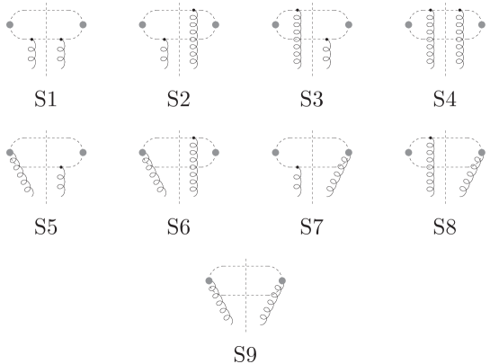
Figure 5: The scalar diagrams for the impact factors.

The scalar part of the impact factor with transversely polarized $R$-currents is

$${\mathchoice{\hbox{$\displaystyle\mathbb{D}$}}{\hbox{$\textstyle\mathbb{D}$}}{\hbox{$\scriptstyle\mathbb{D}$}}{\hbox{$\scriptscriptstyle\mathbb{D}$}}}_{S,(2;0)}^{a_{1}a_{2},hh^{\prime}}({\bf k_{1}},{\bf k_{2}}) = {}2\delta_{a_{1}a_{2}}\,N_{c}\alpha_{s}\int_{0}^{1}d\alpha\int\frac{d^{2}{{\bf l}}}{(2\pi)^{2}}\,\alpha(1-\alpha)$$ (23)

$${}\times\,{\mbox{\boldmath$\epsilon$}}^{(h)}\cdot\left(\frac{\mbox{\boldmath$N$}_{1}}{D_{1}}-\frac{\mbox{\boldmath$N$}_{2}}{D_{2}}\right)\left(\frac{\mbox{\boldmath$N$}_{1}^{\prime}}{D_{1}^{\prime}}-\frac{\mbox{\boldmath$N$}_{2}^{\prime}}{D_{2}^{\prime}}\right)\cdot{\mbox{\boldmath$\epsilon$}}^{(h^{\prime})*}$$

with the propagators and numerators given in (21). The trace over the $\text{SU}_{R}(4)$ generators for scalars in the vector representation, that is included here, gives

$$\mbox{tr}\,_{6}(T^{A}T^{A})=1\,,$$ (24)

different from the fermionic case. Also the scalar contribution ${\mathchoice{\hbox{$\displaystyle\mathbb{D}$}}{\hbox{$\textstyle\mathbb{D}$}}{\hbox{$\scriptstyle\mathbb{D}$}}{\hbox{$\scriptscriptstyle\mathbb{D}$}}}_{S,(2;0)}({\bf k}_{1},{\bf k}_{2})$ to the impact factor is symmetric in its two momentum arguments and vanishes if one of them vanishes ($i\in\{1,2\}$):

$$\left.{\mathchoice{\hbox{$\displaystyle\mathbb{D}$}}{\hbox{$\textstyle\mathbb{D}$}}{\hbox{$\scriptstyle\mathbb{D}$}}{\hbox{$\scriptscriptstyle\mathbb{D}$}}}_{S,(2;0)}^{a_{1}a_{2},hh^{\prime}}({\bf k}_{1},{\bf k}_{2})\right|_{{\bf k}_{i}=0}=0\,.$$ (25)

We obtain the full impact factor in ${\cal N}=4$ SYM as

$${\mathchoice{\hbox{$\displaystyle\mathbb{D}$}}{\hbox{$\textstyle\mathbb{D}$}}{\hbox{$\scriptstyle\mathbb{D}$}}{\hbox{$\scriptscriptstyle\mathbb{D}$}}}^{a_{1}a_{2},hh^{\prime}}_{(2;0)}\equiv{\mathchoice{\hbox{$\displaystyle\mathbb{D}$}}{\hbox{$\textstyle\mathbb{D}$}}{\hbox{$\scriptstyle\mathbb{D}$}}{\hbox{$\scriptscriptstyle\mathbb{D}$}}}^{a_{1}a_{2},hh^{\prime}}_{F,(2;0)}+{\mathchoice{\hbox{$\displaystyle\mathbb{D}$}}{\hbox{$\textstyle\mathbb{D}$}}{\hbox{$\scriptstyle\mathbb{D}$}}{\hbox{$\scriptscriptstyle\mathbb{D}$}}}^{a_{1}a_{2},hh^{\prime}}_{S,(2;0)}\,,$$ (26)

and obtain for the example of transversely polarized $R$-currents

$${\mathchoice{\hbox{$\displaystyle\mathbb{D}$}}{\hbox{$\textstyle\mathbb{D}$}}{\hbox{$\scriptstyle\mathbb{D}$}}{\hbox{$\scriptscriptstyle\mathbb{D}$}}}^{a_{1}a_{2},hh^{\prime}}_{(2;0)}=\delta_{a_{1}a_{2}}\delta_{hh^{\prime}}\frac{N_{c}\alpha_{s}}{2}\int_{0}^{1}d\alpha\int\frac{d^{2}{\bf l}}{(2\pi)^{2}}\left(\frac{\mbox{\boldmath$N$}_{1}}{D_{1}}-\frac{\mbox{\boldmath$N$}_{2}}{D_{2}}\right)\cdot\left(\frac{\mbox{\boldmath$N$}_{1}^{\prime}}{D_{1}^{\prime}}-\frac{\mbox{\boldmath$N$}_{2}^{\prime}}{D_{2}^{\prime}}\right)\,.$$ (27)

${\mathchoice{\hbox{$\displaystyle\mathbb{D}$}}{\hbox{$\textstyle\mathbb{D}$}}{\hbox{$\scriptstyle\mathbb{D}$}}{\hbox{$\scriptscriptstyle\mathbb{D}$}}}_{(2;0)}$ is symmetric in its two momentum arguments, and as a consequence of (22) and (25) we have

$$\left.{\mathchoice{\hbox{$\displaystyle\mathbb{D}$}}{\hbox{$\textstyle\mathbb{D}$}}{\hbox{$\scriptstyle\mathbb{D}$}}{\hbox{$\scriptscriptstyle\mathbb{D}$}}}_{(2;0)}^{a_{1}a_{2},hh^{\prime}}({\bf k}_{1},{\bf k}_{2})\right|_{{\bf k}_{i}=0}=0\,.$$ (28)

It has been observed in [34] that due to supersymmetry the helicities of the scattering $R$-currents are conserved. In particular, unlike the QCD case, helicity conservation holds for the $R$-current impact factor also in the non-forward direction $t\neq 0$. In the following we will keep in our notation the different polarizations $\lambda_{A}$ and $\lambda_{A^{\prime}}$ explicit, while we keep in mind that the impact factor is always proportional to $\delta^{\lambda_{A}\lambda_{A^{\prime}}}$. This also justifies a posteriori the use of the analytic representation (6) for the analysis of the six point function (2.2).

3.2 Six-point functions in ${\cal N}=4$ SYM

The next step is to go to higher correlation functions, e. g. six-point functions (2.2). Again fermions and scalars contribute to the impact factor ${\mathchoice{\hbox{$\displaystyle\mathbb{D}$}}{\hbox{$\textstyle\mathbb{D}$}}{\hbox{$\scriptstyle\mathbb{D}$}}{\hbox{$\scriptscriptstyle\mathbb{D}$}}}_{(n;0)}$. They generalize (16) to an arbitrary number of gluons and are defined as

$$\begin{split}{\mathchoice{\hbox{$\displaystyle\mathbb{D}$}}{\hbox{$\textstyle\mathbb{D}$}}{\hbox{$\scriptstyle\mathbb{D}$}}{\hbox{$\scriptscriptstyle\mathbb{D}$}}}&{}_{(n;0)}^{a_{1}a_{2}\ldots a_{n},\lambda_{A}\lambda_{A^{\prime}}}({\bf k}_{1},\ldots,{\bf k}_{n})\\ &=\frac{p_{B}^{\rho_{1}}\ldots p_{B}^{\rho_{n}}}{s^{n}}\int_{0}^{\infty}\frac{d\tilde{s}_{1}}{2\pi}\ldots\int_{0}^{\infty}\frac{d\tilde{s}_{n-1}}{2\pi}\,\text{disc}_{\tilde{s}_{1}}\ldots\text{disc}_{\tilde{s}_{n-1}}A^{\mu_{A}\mu_{A^{\prime}},\rho_{1}\ldots\rho_{n};a_{1}\ldots a_{n}}_{R_{A}g_{1}\to R_{A^{\prime}}g_{2}\ldots g_{n}}\epsilon^{\lambda_{A}}_{\mu_{A}}(q)\epsilon^{\lambda_{A^{\prime}}}_{\mu_{A^{\prime}}}(q^{\prime})\,,\end{split}$$ (29)

with $\tilde{s}_{i}=(q-\sum_{j=1}^{i}k_{j})^{2}$, $i=1,\ldots n-1$. One possible diagram with fermion loops contributing to the six-point function is depicted in figure 6. The complete impact factors are again given by the sum over all possible ways in which the gluons can couple to the fermion and scalar lines.

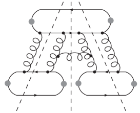
Figure 6: A fermionic contribution to the six-point function

In the following discussion of amplitudes with more gluons the color factors will play a crucial role, in particular when we explain how amplitudes with different numbers of gluons are related to each other via reggeization. We will invoke known results from QCD in order to derive these relations for the case of ${\cal N}=4$ SYM. When comparing the fermionic contributions we will always find the overall factor $R$ of (18) when comparing an ${\cal N}=4$ SYM amplitude to its analog in QCD. The color factor, on the other hand, will have a richer structure, such that the main structural difference between the two theories originates from the color representations of the particles. In the following we will therefore sometimes (in slight abuse of language) speak of the ‘adjoint’ and ‘fundamental’ representation when we actually refer to ${\cal N}=4$ SYM and QCD, respectively. In fact, the results obtained below for the fermions can be used for considering a theory like QCD with adjoint instead of fundamental quarks by just dropping the factor $R$ wherever it occurs.

3.2.1 Fermionic impact factor

For the case of fundamental quarks in QCD the impact factors with up to six gluons have been given explicitly in [8, 9]. There it has been found that the impact factors with arbitrarily many gluons can be related to the two-gluon impact factor $D_{(2;0)}$. A detailed account of how this reggeization of the impact factors results from the corresponding diagrams has been given in [41]. Here we want to relate the Weyl fermion impact factors in the adjoint representation to those of the fundamental representation. In accordance with the notation of the previous section we assign color labels $a_{i}$ and transverse momenta ${\bf k}_{i}$ to the gluons.

To understand the main difference between QCD and ${\cal N}=4$ SYM we have to take a closer look at the traces in color space. Inspection of the possible diagrams contributing to the $n$-gluon impact factor shows that these diagrams come in pairs: for each diagram there is another diagram with the same momentum integration but with the generators occurring in opposite order in the trace in color space. The relative sign between these two diagrams turns out to be positive for even numbers of gluons and negative for odd numbers of gluons. It further turns out that the full impact factors can be written completely in terms of the momentum part of the two-gluon impact factor, see [8, 9]. (In that representation the diagrams with all gluons attached to the same quark line occur several times with different color factors but cancel in the sum over two-gluon impact factors such that the original two diagrams of this type are correctly counted.) It is straightforward to check, following for example the derivation presented in [41], that this result holds also in the case of adjoint fermions.

Let us first define the momentum part of the two-gluon amplitude by separating it from the color tensor,

$$D_{(2;0)}^{a_{1}a_{2}}({\bf k}_{1},{\bf k}_{2})=\delta_{a_{1}a_{2}}D_{(2;0)}({\bf k}_{1},{\bf k}_{2})\,,$$ (30)

and analogously for ${\mathchoice{\hbox{$\displaystyle\mathbb{D}$}}{\hbox{$\textstyle\mathbb{D}$}}{\hbox{$\scriptstyle\mathbb{D}$}}{\hbox{$\scriptscriptstyle\mathbb{D}$}}}_{(2;0)}^{a_{1}a_{2}}$.

For three gluons a pair of diagrams as described above comes with the difference of two traces over generators of the respective representation. For the adjoint representation we have for instance

$$\mbox{tr}\,(T^{a_{1}}T^{a_{2}}T^{a_{3}})-\mbox{tr}\,(T^{a_{3}}T^{a_{2}}T^{a_{1}})=iN_{c}f_{a_{1}a_{2}a_{3}}\,,$$ (31)

while in the fundamental representation (i. e. in QCD) we had

$$\mbox{tr}\,(t^{a_{1}}t^{a_{2}}t^{a_{3}})-\mbox{tr}\,(t^{a_{3}}t^{a_{2}}t^{a_{1}})=\frac{i}{2}f_{a_{1}a_{2}a_{3}}$$ (32)

instead, giving again rise to a relative factor $2N_{c}R$ in the ${\cal N}=4$ SYM case as compared to the QCD case. This applies to all pairs of diagrams. Invoking the known decomposition of the fundamental impact factor $D_{(3;0)}$ into a sum over $D_{(2;0)}$ [7, 8],

$$D_{(3;0)}^{a_{1}a_{2}a_{3}}({\bf k}_{1},{\bf k}_{2},{\bf k}_{3})=\frac{1}{2}gf_{a_{1}a_{2}a_{3}}\,[D_{(2;0)}(12,3)-D_{(2;0)}(13,2)+D_{(2;0)}(1,23)]\,,$$ (33)

we find for the adjoint representation in ${\cal N}=4$ SYM

$$\begin{split}{\mathchoice{\hbox{$\displaystyle\mathbb{D}$}}{\hbox{$\textstyle\mathbb{D}$}}{\hbox{$\scriptstyle\mathbb{D}$}}{\hbox{$\scriptscriptstyle\mathbb{D}$}}}_{F,(3;0)}^{a_{1}a_{2}a_{3}}({\bf k}_{1},{\bf k}_{2},{\bf k}_{3})&=2N_{c}R\,D_{(3;0)}^{a_{1}a_{2}a_{3}}({\bf k}_{1},{\bf k}_{2},{\bf k}_{3})\\ &=\frac{1}{2}gf_{a_{1}a_{2}a_{3}}\,[{\mathchoice{\hbox{$\displaystyle\mathbb{D}$}}{\hbox{$\textstyle\mathbb{D}$}}{\hbox{$\scriptstyle\mathbb{D}$}}{\hbox{$\scriptscriptstyle\mathbb{D}$}}}_{F,(2;0)}(12,3)-{\mathchoice{\hbox{$\displaystyle\mathbb{D}$}}{\hbox{$\textstyle\mathbb{D}$}}{\hbox{$\scriptstyle\mathbb{D}$}}{\hbox{$\scriptscriptstyle\mathbb{D}$}}}_{F,(2;0)}(13,2)+{\mathchoice{\hbox{$\displaystyle\mathbb{D}$}}{\hbox{$\textstyle\mathbb{D}$}}{\hbox{$\scriptstyle\mathbb{D}$}}{\hbox{$\scriptscriptstyle\mathbb{D}$}}}_{F,(2;0)}(1,23)]\,.\end{split}$$ (34)

Here we have made use of the shorthand notation for the momentum arguments of ${\mathchoice{\hbox{$\displaystyle\mathbb{D}$}}{\hbox{$\textstyle\mathbb{D}$}}{\hbox{$\scriptstyle\mathbb{D}$}}{\hbox{$\scriptscriptstyle\mathbb{D}$}}}_{(2;0)}$ and $D_{(2;0)}$ originally introduced in [9] in which the momenta are replaced by their indices, and a string of indices stands for the sum of momenta, for example

$$D_{(2;0)}(12,3)=D_{(2;0)}({\bf k}_{1}+{\bf k}_{2},{\bf k}_{3})\,.$$ (35)

In the following this notation will also be used for other functions. Note that we have expressed both three-gluon impact factors here in terms of the momentum part of the two-gluon impact factor which does no longer contain the color factor $\delta_{ab}$. We observe that the three-gluon impact factor in the adjoint representation (34) differs from the one in the fundamental representation (33) only by a factor $2N_{c}R$. As a consequence the relation between the three-gluon impact factor and the corresponding two-gluon impact factor is the same in both representations, compare the second line of (34) with (33). What we observe here is the reggeization of the gluon in the impact factor. In each term in the sum in (34) or (33) two gluons combine to act as a single gluon.

For four gluons the situation becomes more interesting. In the fundamental representation, the color structure of a typical pair of diagrams with the same momentum structure is given by the tensor

$$d^{abcd}=\mbox{tr}\,(t^{a}t^{b}t^{c}t^{d})+\mbox{tr}\,(t^{d}t^{c}t^{b}t^{a})\,.$$ (36)

Taking the quarks to be in the adjoint representation gives us the same two traces with the fundamental generators $t^{a}$ replaced by adjoint generators $T^{a}$,

$$\mbox{tr}\,(T^{a}T^{b}T^{c}T^{d})+\mbox{tr}\,(T^{d}T^{c}T^{b}T^{a})=2N_{c}d^{abcd}+\delta_{ab}\delta_{cd}+\delta_{ac}\delta_{bd}+\delta_{ad}\delta_{bc}\,,$$ (37)

where we have used (102) and (104) in order to express this sum of traces in terms of the tensor in (36) known from the fundamental representation. We notice that in the case of four gluons we find a further part in addition to reproducing $2N_{c}$ times the tensor from the fundamental representation. Using the known result for the four-gluon impact factor in the fundamental representation [8],

$$D_{(4;0)}^{a_{1}a_{2}a_{3}a_{4}}({\bf k}_{1},{\bf k}_{2},{\bf k}_{3},{\bf k}_{4}) = {}-g^{2}d^{a_{1}a_{2}a_{3}a_{4}}\,[D_{(2;0)}(123,4)+D_{(2;0)}(1,234)-D_{(2;0)}(14,23)]$$ (38)

$${}-g^{2}d^{a_{2}a_{1}a_{3}a_{4}}\,[D_{(2;0)}(134,2)+D_{(2;0)}(124,3)-D_{(2;0)}(12,34)$$

$${}\hskip 68.28644pt-D_{(2;0)}(13,24)]\,,$$

and (37) we hence arrive at

$${\mathchoice{\hbox{$\displaystyle\mathbb{D}$}}{\hbox{$\textstyle\mathbb{D}$}}{\hbox{$\scriptstyle\mathbb{D}$}}{\hbox{$\scriptscriptstyle\mathbb{D}$}}}_{F,(4;0)}^{a_{1}a_{2}a_{3}a_{4}}({\bf k}_{1},{\bf k}_{2},{\bf k}_{3},{\bf k}_{4})$$ (39)

$$= {}2N_{c}R\,D_{(4;0)}^{a_{1}a_{2}a_{3}a_{4}}({\bf k}_{1},{\bf k}_{2},{\bf k}_{3},{\bf k}_{4})+{\mathchoice{\hbox{$\displaystyle\mathbb{D}$}}{\hbox{$\textstyle\mathbb{D}$}}{\hbox{$\scriptstyle\mathbb{D}$}}{\hbox{$\scriptscriptstyle\mathbb{D}$}}}^{a_{1}a_{2}a_{3}a_{4}}_{F,(4;0)\,\text{dir}}({\bf k}_{1},{\bf k}_{2},{\bf k}_{3},{\bf k}_{4})$$

$$= {}-g^{2}d^{a_{1}a_{2}a_{3}a_{4}}\,[{\mathchoice{\hbox{$\displaystyle\mathbb{D}$}}{\hbox{$\textstyle\mathbb{D}$}}{\hbox{$\scriptstyle\mathbb{D}$}}{\hbox{$\scriptscriptstyle\mathbb{D}$}}}_{F,(2;0)}(123,4)+{\mathchoice{\hbox{$\displaystyle\mathbb{D}$}}{\hbox{$\textstyle\mathbb{D}$}}{\hbox{$\scriptstyle\mathbb{D}$}}{\hbox{$\scriptscriptstyle\mathbb{D}$}}}_{F,(2;0)}(1,234)-{\mathchoice{\hbox{$\displaystyle\mathbb{D}$}}{\hbox{$\textstyle\mathbb{D}$}}{\hbox{$\scriptstyle\mathbb{D}$}}{\hbox{$\scriptscriptstyle\mathbb{D}$}}}_{F,(2;0)}(14,23)]$$

$${}-g^{2}d^{a_{2}a_{1}a_{3}a_{4}}\,[{\mathchoice{\hbox{$\displaystyle\mathbb{D}$}}{\hbox{$\textstyle\mathbb{D}$}}{\hbox{$\scriptstyle\mathbb{D}$}}{\hbox{$\scriptscriptstyle\mathbb{D}$}}}_{F,(2;0)}(134,2)+{\mathchoice{\hbox{$\displaystyle\mathbb{D}$}}{\hbox{$\textstyle\mathbb{D}$}}{\hbox{$\scriptstyle\mathbb{D}$}}{\hbox{$\scriptscriptstyle\mathbb{D}$}}}_{F,(2;0)}(124,3)-{\mathchoice{\hbox{$\displaystyle\mathbb{D}$}}{\hbox{$\textstyle\mathbb{D}$}}{\hbox{$\scriptstyle\mathbb{D}$}}{\hbox{$\scriptscriptstyle\mathbb{D}$}}}_{F,(2;0)}(12,34)-{\mathchoice{\hbox{$\displaystyle\mathbb{D}$}}{\hbox{$\textstyle\mathbb{D}$}}{\hbox{$\scriptstyle\mathbb{D}$}}{\hbox{$\scriptscriptstyle\mathbb{D}$}}}_{F,(2;0)}(13,24)]$$

$${}+{\mathchoice{\hbox{$\displaystyle\mathbb{D}$}}{\hbox{$\textstyle\mathbb{D}$}}{\hbox{$\scriptstyle\mathbb{D}$}}{\hbox{$\scriptscriptstyle\mathbb{D}$}}}^{a_{1}a_{2}a_{3}a_{4}}_{F,(4;0)\,\text{dir}}(1,2,3,4)\,.$$

Here the additional part ${\mathchoice{\hbox{$\displaystyle\mathbb{D}$}}{\hbox{$\textstyle\mathbb{D}$}}{\hbox{$\scriptstyle\mathbb{D}$}}{\hbox{$\scriptscriptstyle\mathbb{D}$}}}_{F,(4;0)\,\text{dir}}$ originates from the additional delta tensors in (37): later on it will be shown that this piece – in contrast to the other terms in eq. (39) – gives rise to a direct coupling of the four-gluon state in the $t$-channel to the external currents. Explicitly, it becomes

$$\begin{split}{\mathchoice{\hbox{$\displaystyle\mathbb{D}$}}{\hbox{$\textstyle\mathbb{D}$}}{\hbox{$\scriptstyle\mathbb{D}$}}{\hbox{$\scriptscriptstyle\mathbb{D}$}}}^{a_{1}a_{2}a_{3}a_{4}}_{F,(4;0)\,\text{dir}}&({\bf k}_{1},{\bf k}_{2},{\bf k}_{3},{\bf k}_{4})\\ =&-g^{2}\frac{1}{2N_{c}}\,(\delta_{a_{1}a_{2}}\delta_{a_{3}a_{4}}+\delta_{a_{1}a_{3}}\delta_{a_{2}a_{4}}+\delta_{a_{1}a_{4}}\delta_{a_{2}a_{3}})\\ &{}\times\left[{\mathchoice{\hbox{$\displaystyle\mathbb{D}$}}{\hbox{$\textstyle\mathbb{D}$}}{\hbox{$\scriptstyle\mathbb{D}$}}{\hbox{$\scriptscriptstyle\mathbb{D}$}}}_{F,(2;0)}(123,4)+{\mathchoice{\hbox{$\displaystyle\mathbb{D}$}}{\hbox{$\textstyle\mathbb{D}$}}{\hbox{$\scriptstyle\mathbb{D}$}}{\hbox{$\scriptscriptstyle\mathbb{D}$}}}_{F,(2;0)}(124,3)+{\mathchoice{\hbox{$\displaystyle\mathbb{D}$}}{\hbox{$\textstyle\mathbb{D}$}}{\hbox{$\scriptstyle\mathbb{D}$}}{\hbox{$\scriptscriptstyle\mathbb{D}$}}}_{F,(2;0)}(134,2)+{\mathchoice{\hbox{$\displaystyle\mathbb{D}$}}{\hbox{$\textstyle\mathbb{D}$}}{\hbox{$\scriptstyle\mathbb{D}$}}{\hbox{$\scriptscriptstyle\mathbb{D}$}}}_{F,(2;0)}(1,234)\right.\\ &{}\left.\hskip 14.22636pt-{\mathchoice{\hbox{$\displaystyle\mathbb{D}$}}{\hbox{$\textstyle\mathbb{D}$}}{\hbox{$\scriptstyle\mathbb{D}$}}{\hbox{$\scriptscriptstyle\mathbb{D}$}}}_{F,(2;0)}(12,34)-{\mathchoice{\hbox{$\displaystyle\mathbb{D}$}}{\hbox{$\textstyle\mathbb{D}$}}{\hbox{$\scriptstyle\mathbb{D}$}}{\hbox{$\scriptscriptstyle\mathbb{D}$}}}_{F,(2;0)}(13,24)-{\mathchoice{\hbox{$\displaystyle\mathbb{D}$}}{\hbox{$\textstyle\mathbb{D}$}}{\hbox{$\scriptstyle\mathbb{D}$}}{\hbox{$\scriptscriptstyle\mathbb{D}$}}}_{F,(2;0)}(14,23)\right]\,.\end{split}$$ (40)

The factor $(2N_{c})^{-1}$ appears because we have expressed the r.h.s. in terms of ${\mathchoice{\hbox{$\displaystyle\mathbb{D}$}}{\hbox{$\textstyle\mathbb{D}$}}{\hbox{$\scriptstyle\mathbb{D}$}}{\hbox{$\scriptscriptstyle\mathbb{D}$}}}_{F,(2;0)}$ instead of $D_{(2;0)}$. Interestingly, due to the symmetry of ${\mathchoice{\hbox{$\displaystyle\mathbb{D}$}}{\hbox{$\textstyle\mathbb{D}$}}{\hbox{$\scriptstyle\mathbb{D}$}}{\hbox{$\scriptscriptstyle\mathbb{D}$}}}_{F,(2;0)}$, this additional term is completely symmetric in its color and momentum arguments. We furthermore observe that due to (28) it vanishes if one of the gluon momenta vanishes, that is for all $i$ we have

$$\left.{\mathchoice{\hbox{$\displaystyle\mathbb{D}$}}{\hbox{$\textstyle\mathbb{D}$}}{\hbox{$\scriptstyle\mathbb{D}$}}{\hbox{$\scriptscriptstyle\mathbb{D}$}}}^{a_{1}a_{2}a_{3}a_{4}}_{F,(4;0)\,\text{dir}}({\bf k}_{1},{\bf k}_{2},{\bf k}_{3},{\bf k}_{4})\right|_{{\bf k}_{i}=0}=0\,.$$ (41)

We will discuss the physical interpretation of this additional piece in section 5 below.

3.2.2 Scalar impact factor

In ${\cal N}=4$ SYM scalars provide a contribution to the full impact factor also for larger numbers of gluons. A scalar contribution to the six-point function is shown in figure 7.

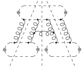
Figure 7: A scalar contribution to the six-point function

In this section we argue that it is possible to relate the scalar impact factors for $n$ gluons, ${\mathchoice{\hbox{$\displaystyle\mathbb{D}$}}{\hbox{$\textstyle\mathbb{D}$}}{\hbox{$\scriptstyle\mathbb{D}$}}{\hbox{$\scriptscriptstyle\mathbb{D}$}}}_{S,(n;0)}$, to the two-gluon impact factor ${\mathchoice{\hbox{$\displaystyle\mathbb{D}$}}{\hbox{$\textstyle\mathbb{D}$}}{\hbox{$\scriptstyle\mathbb{D}$}}{\hbox{$\scriptscriptstyle\mathbb{D}$}}}_{S,(2;0)}$ in the same way as for fermions.

Additional diagrams like S5-S9 for the two-point function in figure 5 also appear with three or more gluons in the $t$-channel, see figure 8. But these diagrams are suppressed for the same reasons as in the case of two $t$-channel gluons. Every contraction of the gluon polarization tensor,

$$g^{\mu\nu}=\frac{2}{s}(p^{\mu}_{B}q^{\nu}_{A}+q_{A}^{\mu}p_{B}^{\nu})+g^{\mu\nu}_{\perp}\,,$$ (42)

with the polarization vector of the $R$-current provides one power of $s$ less than in the leading diagrams. Therefore at high energies only diagrams with gluons coupled directly to the scalar lines contribute to the scalar impact factor.

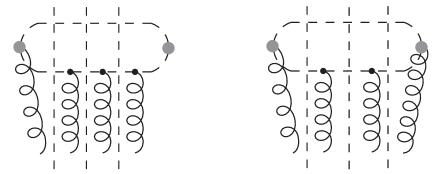
Figure 8: Two of the additional diagrams in the scalar case

Furthermore, diagrams as the one shown in figure 9 do not contribute to the discontinuity that we are considering.

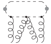
Figure 9: A further scalar diagram

Because of the suppression of the additional diagrams also in the scalar part all impact factors ${\mathchoice{\hbox{$\displaystyle\mathbb{D}$}}{\hbox{$\textstyle\mathbb{D}$}}{\hbox{$\scriptstyle\mathbb{D}$}}{\hbox{$\scriptscriptstyle\mathbb{D}$}}}_{S,(n;0)}$ with arbitrarily many gluons can be expressed in terms of the two-gluon impact factor ${\mathchoice{\hbox{$\displaystyle\mathbb{D}$}}{\hbox{$\textstyle\mathbb{D}$}}{\hbox{$\scriptstyle\mathbb{D}$}}{\hbox{$\scriptscriptstyle\mathbb{D}$}}}_{S,(2;0)}$. The reduction mechanism is similar to the one with fermion loops. The key mechanism for fermions has been explained for example in [9], here we will now consider it for scalars.

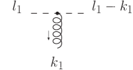
Figure 10: Scalar-gluon vertex

A scalar-gluon vertex, figure 10, contracted with the leading longitudinal part of the gluon polarization tensor (42), $2p_{B}^{\mu}q_{A}^{\nu}/s$, is proportional to $s\alpha$, where again we make use of a Sudakov decomposition $l=\alpha q_{A}+\beta p_{B}+l_{t}$ (as in (5)) of the loop momentum of the scalar loop. Let us now consider two adjacent gluons out of the $n$ gluons which couple to the scalar loop. Every scalar-gluon vertex is contracted with the longitudinal momentum $p_{B}$ from the polarization tensor of the $t$-channel gluon. Furthermore, the scalar propagator is on-shell, thus resulting in a delta function. Then we obtain

$$\hbox{\raise-22.37854pt\hbox{\includegraphics[width=128.0374pt]{sred.eps}}}\simeq\,\,\,\alpha s(l-k_{1}+l-k_{1}-k_{2})\!\cdot\!p_{B}\,\,2\pi\delta((l-k_{1})^{2})\,.$$ (43)

Making use of the Sudakov decomposition we find

$$\alpha\,s\,\delta\left((\beta-\beta_{k_{1}})-{({\bf l}-{\bf k}_{1})^{2}}/{s\alpha}\right)\,\,\sim\hbox{\raise-27.82394pt\hbox{\includegraphics[width=128.0374pt]{sred2.eps}}}$$ (44)

which is the same as the one-gluon-scalar vertex, but with the transverse momentum given by the sum of the momenta of both $t$-channel gluons. This means that we observe reggeization of the gluons in the scalar part of the impact factor as well.

The scalar diagrams contributing to the impact factor come in pairs exactly as the fermionic ones. The two diagrams in each pair have the same momentum structure but the color trace occurs in reversed order. The relative sign between these two diagrams is again $(-1)^{n}$ where $n$ is the number of gluons.

Altogether, the decomposition of the scalar impact factors ${\mathchoice{\hbox{$\displaystyle\mathbb{D}$}}{\hbox{$\textstyle\mathbb{D}$}}{\hbox{$\scriptstyle\mathbb{D}$}}{\hbox{$\scriptscriptstyle\mathbb{D}$}}}_{S,(n;0)}$ into a sum of ${\mathchoice{\hbox{$\displaystyle\mathbb{D}$}}{\hbox{$\textstyle\mathbb{D}$}}{\hbox{$\scriptstyle\mathbb{D}$}}{\hbox{$\scriptscriptstyle\mathbb{D}$}}}_{S,(2;0)}$ works in the same way as for fermions. The results are

$${\mathchoice{\hbox{$\displaystyle\mathbb{D}$}}{\hbox{$\textstyle\mathbb{D}$}}{\hbox{$\scriptstyle\mathbb{D}$}}{\hbox{$\scriptscriptstyle\mathbb{D}$}}}_{S,(3;0)}^{a_{1}a_{2}a_{3}}({\bf k}_{1},{\bf k}_{2},{\bf k}_{3}) = {}\frac{1}{2}gf_{a_{1}a_{2}a_{3}}\,[{\mathchoice{\hbox{$\displaystyle\mathbb{D}$}}{\hbox{$\textstyle\mathbb{D}$}}{\hbox{$\scriptstyle\mathbb{D}$}}{\hbox{$\scriptscriptstyle\mathbb{D}$}}}_{S,(2;0)}(12,3)-{\mathchoice{\hbox{$\displaystyle\mathbb{D}$}}{\hbox{$\textstyle\mathbb{D}$}}{\hbox{$\scriptstyle\mathbb{D}$}}{\hbox{$\scriptscriptstyle\mathbb{D}$}}}_{S,(2;0)}(13,2)+{\mathchoice{\hbox{$\displaystyle\mathbb{D}$}}{\hbox{$\textstyle\mathbb{D}$}}{\hbox{$\scriptstyle\mathbb{D}$}}{\hbox{$\scriptscriptstyle\mathbb{D}$}}}_{S,(2;0)}(1,23)]$$ (45)

and

$${\mathchoice{\hbox{$\displaystyle\mathbb{D}$}}{\hbox{$\textstyle\mathbb{D}$}}{\hbox{$\scriptstyle\mathbb{D}$}}{\hbox{$\scriptscriptstyle\mathbb{D}$}}}_{S,(4;0)}^{a_{1}a_{2}a_{3}a_{4}}({\bf k}_{1},{\bf k}_{2},{\bf k}_{3},{\bf k}_{4})$$ (46)

$$= {}-g^{2}d^{a_{1}a_{2}a_{3}a_{4}}\,[{\mathchoice{\hbox{$\displaystyle\mathbb{D}$}}{\hbox{$\textstyle\mathbb{D}$}}{\hbox{$\scriptstyle\mathbb{D}$}}{\hbox{$\scriptscriptstyle\mathbb{D}$}}}_{S,(2;0)}(123,4)+{\mathchoice{\hbox{$\displaystyle\mathbb{D}$}}{\hbox{$\textstyle\mathbb{D}$}}{\hbox{$\scriptstyle\mathbb{D}$}}{\hbox{$\scriptscriptstyle\mathbb{D}$}}}_{S,(2;0)}(1,234)-{\mathchoice{\hbox{$\displaystyle\mathbb{D}$}}{\hbox{$\textstyle\mathbb{D}$}}{\hbox{$\scriptstyle\mathbb{D}$}}{\hbox{$\scriptscriptstyle\mathbb{D}$}}}_{S,(2;0)}(14,23)]$$

$${}-g^{2}d^{a_{2}a_{1}a_{3}a_{4}}\,[{\mathchoice{\hbox{$\displaystyle\mathbb{D}$}}{\hbox{$\textstyle\mathbb{D}$}}{\hbox{$\scriptstyle\mathbb{D}$}}{\hbox{$\scriptscriptstyle\mathbb{D}$}}}_{S,(2;0)}(134,2)+{\mathchoice{\hbox{$\displaystyle\mathbb{D}$}}{\hbox{$\textstyle\mathbb{D}$}}{\hbox{$\scriptstyle\mathbb{D}$}}{\hbox{$\scriptscriptstyle\mathbb{D}$}}}_{S,(2;0)}(124,3)-{\mathchoice{\hbox{$\displaystyle\mathbb{D}$}}{\hbox{$\textstyle\mathbb{D}$}}{\hbox{$\scriptstyle\mathbb{D}$}}{\hbox{$\scriptscriptstyle\mathbb{D}$}}}_{S,(2;0)}(12,34)-{\mathchoice{\hbox{$\displaystyle\mathbb{D}$}}{\hbox{$\textstyle\mathbb{D}$}}{\hbox{$\scriptstyle\mathbb{D}$}}{\hbox{$\scriptscriptstyle\mathbb{D}$}}}_{S,(2;0)}(13,24)]$$

$${}+{\mathchoice{\hbox{$\displaystyle\mathbb{D}$}}{\hbox{$\textstyle\mathbb{D}$}}{\hbox{$\scriptstyle\mathbb{D}$}}{\hbox{$\scriptscriptstyle\mathbb{D}$}}}^{a_{1}a_{2}a_{3}a_{4}}_{S,(4;0)\,\text{dir}}(1,2,3,4)\,,$$

with ${\mathchoice{\hbox{$\displaystyle\mathbb{D}$}}{\hbox{$\textstyle\mathbb{D}$}}{\hbox{$\scriptstyle\mathbb{D}$}}{\hbox{$\scriptscriptstyle\mathbb{D}$}}}^{a_{1}a_{2}a_{3}a_{4}}_{S,(4;0)\,\text{dir}}(1,2,3,4)$ as in eq. (40) but with the index $F$ replaced by $S$ in all terms.

The full impact factors ${\mathchoice{\hbox{$\displaystyle\mathbb{D}$}}{\hbox{$\textstyle\mathbb{D}$}}{\hbox{$\scriptstyle\mathbb{D}$}}{\hbox{$\scriptscriptstyle\mathbb{D}$}}}_{(3;0)}$ and ${\mathchoice{\hbox{$\displaystyle\mathbb{D}$}}{\hbox{$\textstyle\mathbb{D}$}}{\hbox{$\scriptstyle\mathbb{D}$}}{\hbox{$\scriptscriptstyle\mathbb{D}$}}}_{(4;0)}$ are then given by the sum of the fermionic and scalar impact factors as in the two-gluon case (27):

$$\begin{split}{\mathchoice{\hbox{$\displaystyle\mathbb{D}$}}{\hbox{$\textstyle\mathbb{D}$}}{\hbox{$\scriptstyle\mathbb{D}$}}{\hbox{$\scriptscriptstyle\mathbb{D}$}}}_{(3;0)}&={\mathchoice{\hbox{$\displaystyle\mathbb{D}$}}{\hbox{$\textstyle\mathbb{D}$}}{\hbox{$\scriptstyle\mathbb{D}$}}{\hbox{$\scriptscriptstyle\mathbb{D}$}}}_{F,(3;0)}+{\mathchoice{\hbox{$\displaystyle\mathbb{D}$}}{\hbox{$\textstyle\mathbb{D}$}}{\hbox{$\scriptstyle\mathbb{D}$}}{\hbox{$\scriptscriptstyle\mathbb{D}$}}}_{S,(3;0)}\\ {\mathchoice{\hbox{$\displaystyle\mathbb{D}$}}{\hbox{$\textstyle\mathbb{D}$}}{\hbox{$\scriptstyle\mathbb{D}$}}{\hbox{$\scriptscriptstyle\mathbb{D}$}}}_{(4;0)}&={\mathchoice{\hbox{$\displaystyle\mathbb{D}$}}{\hbox{$\textstyle\mathbb{D}$}}{\hbox{$\scriptstyle\mathbb{D}$}}{\hbox{$\scriptscriptstyle\mathbb{D}$}}}_{F,(4;0)}+{\mathchoice{\hbox{$\displaystyle\mathbb{D}$}}{\hbox{$\textstyle\mathbb{D}$}}{\hbox{$\scriptstyle\mathbb{D}$}}{\hbox{$\scriptscriptstyle\mathbb{D}$}}}_{S,(4;0)}\,.\end{split}$$ (47)

This holds for arbitrary polarization of the $R$-currents.

The key result of the present section is that we have been able to express the fermionic parts of the adjoint (${\cal N}=4$) impact factors with up to four gluons attached in terms of the corresponding fundamental (QCD) impact factors and in terms of one new element, namely the additional piece ${\mathchoice{\hbox{$\displaystyle\mathbb{D}$}}{\hbox{$\textstyle\mathbb{D}$}}{\hbox{$\scriptstyle\mathbb{D}$}}{\hbox{$\scriptscriptstyle\mathbb{D}$}}}_{F,(4;0)\,\text{dir}}$. The parts that could be related to the fundamental impact factors can also be expressed in terms of the adjoint two-gluon impact factor ${\mathchoice{\hbox{$\displaystyle\mathbb{D}$}}{\hbox{$\textstyle\mathbb{D}$}}{\hbox{$\scriptstyle\mathbb{D}$}}{\hbox{$\scriptscriptstyle\mathbb{D}$}}}_{F,(2;0)}$ in exactly the same way as the fundamental impact factors could be expressed in terms of $D_{(2;0)}$. For the scalar contributions to the ${\cal N}=4$ impact factors, that is absent in QCD, we find an analogous situation. The $n$-gluon impact factors ${\mathchoice{\hbox{$\displaystyle\mathbb{D}$}}{\hbox{$\textstyle\mathbb{D}$}}{\hbox{$\scriptstyle\mathbb{D}$}}{\hbox{$\scriptscriptstyle\mathbb{D}$}}}_{S,(n;0)}$ can be expressed in terms of the two-gluon impact factor ${\mathchoice{\hbox{$\displaystyle\mathbb{D}$}}{\hbox{$\textstyle\mathbb{D}$}}{\hbox{$\scriptstyle\mathbb{D}$}}{\hbox{$\scriptscriptstyle\mathbb{D}$}}}_{S,(2;0)}$ and in terms of a new element ${\mathchoice{\hbox{$\displaystyle\mathbb{D}$}}{\hbox{$\textstyle\mathbb{D}$}}{\hbox{$\scriptstyle\mathbb{D}$}}{\hbox{$\scriptscriptstyle\mathbb{D}$}}}_{S,(4;0)\,\text{dir}}$ which occurs for four gluons. The relations in the fermionic and in the scalar sector are completely analogous so that they also hold for the full impact factors ${\mathchoice{\hbox{$\displaystyle\mathbb{D}$}}{\hbox{$\textstyle\mathbb{D}$}}{\hbox{$\scriptstyle\mathbb{D}$}}{\hbox{$\scriptscriptstyle\mathbb{D}$}}}_{(n;0)}$. In section 5 we will use this observation to extract the structure of the solutions to the integral equations in a simple way.

It is interesting to note that the pattern of reggeization, found for ${\mathchoice{\hbox{$\displaystyle\mathbb{D}$}}{\hbox{$\textstyle\mathbb{D}$}}{\hbox{$\scriptstyle\mathbb{D}$}}{\hbox{$\scriptscriptstyle\mathbb{D}$}}}_{(2;0)}$, ${\mathchoice{\hbox{$\displaystyle\mathbb{D}$}}{\hbox{$\textstyle\mathbb{D}$}}{\hbox{$\scriptstyle\mathbb{D}$}}{\hbox{$\scriptscriptstyle\mathbb{D}$}}}_{(3;0)}$, and ${\mathchoice{\hbox{$\displaystyle\mathbb{D}$}}{\hbox{$\textstyle\mathbb{D}$}}{\hbox{$\scriptstyle\mathbb{D}$}}{\hbox{$\scriptscriptstyle\mathbb{D}$}}}_{(4;0)}$, continues for more than 4 gluons. Similar to ${\mathchoice{\hbox{$\displaystyle\mathbb{D}$}}{\hbox{$\textstyle\mathbb{D}$}}{\hbox{$\scriptstyle\mathbb{D}$}}{\hbox{$\scriptscriptstyle\mathbb{D}$}}}_{(3;0)}$ which, via reggeization, can be expressed in terms of a sum of ${\mathchoice{\hbox{$\displaystyle\mathbb{D}$}}{\hbox{$\textstyle\mathbb{D}$}}{\hbox{$\scriptstyle\mathbb{D}$}}{\hbox{$\scriptscriptstyle\mathbb{D}$}}}_{(2;0)}$ impact factors, the five-gluon impact factor, ${\mathchoice{\hbox{$\displaystyle\mathbb{D}$}}{\hbox{$\textstyle\mathbb{D}$}}{\hbox{$\scriptstyle\mathbb{D}$}}{\hbox{$\scriptscriptstyle\mathbb{D}$}}}_{(5;0)}$, can be expressed in terms of lower impact factors. In particular, we find the new term ${\mathchoice{\hbox{$\displaystyle\mathbb{D}$}}{\hbox{$\textstyle\mathbb{D}$}}{\hbox{$\scriptstyle\mathbb{D}$}}{\hbox{$\scriptscriptstyle\mathbb{D}$}}}_{(5;0)\,\text{dir}}$ which can be expressed in terms of the analogous four-gluon piece, ${\mathchoice{\hbox{$\displaystyle\mathbb{D}$}}{\hbox{$\textstyle\mathbb{D}$}}{\hbox{$\scriptstyle\mathbb{D}$}}{\hbox{$\scriptscriptstyle\mathbb{D}$}}}_{(4;0)\,\text{dir}}$. More precisely, defining

$${\mathchoice{\hbox{$\displaystyle\mathbb{D}$}}{\hbox{$\textstyle\mathbb{D}$}}{\hbox{$\scriptstyle\mathbb{D}$}}{\hbox{$\scriptscriptstyle\mathbb{D}$}}}_{(4;0)\,\text{dir}}={\mathchoice{\hbox{$\displaystyle\mathbb{D}$}}{\hbox{$\textstyle\mathbb{D}$}}{\hbox{$\scriptstyle\mathbb{D}$}}{\hbox{$\scriptscriptstyle\mathbb{D}$}}}_{F,(4;0)\,\text{dir}}+{\mathchoice{\hbox{$\displaystyle\mathbb{D}$}}{\hbox{$\textstyle\mathbb{D}$}}{\hbox{$\scriptstyle\mathbb{D}$}}{\hbox{$\scriptscriptstyle\mathbb{D}$}}}_{S,(4;0)\,\text{dir}}\,,$$ (48)

we find that

$${\mathchoice{\hbox{$\displaystyle\mathbb{D}$}}{\hbox{$\textstyle\mathbb{D}$}}{\hbox{$\scriptstyle\mathbb{D}$}}{\hbox{$\scriptscriptstyle\mathbb{D}$}}}^{a_{1}a_{2}a_{3}a_{4}a_{5}}_{(5;0)\,\text{dir}}({\bf k}_{1},{\bf k}_{2},{\bf k}_{3},{\bf k}_{4},{\bf k}_{5})$$ (49)

$$= {}\frac{g}{2}\left[f_{a_{1}a_{2}c}\,{\mathchoice{\hbox{$\displaystyle\mathbb{D}$}}{\hbox{$\textstyle\mathbb{D}$}}{\hbox{$\scriptstyle\mathbb{D}$}}{\hbox{$\scriptscriptstyle\mathbb{D}$}}}_{(4;0)\text{dir}}^{ca_{3}a_{4}a_{5}}(12,3,4,5)+f_{a_{1}a_{3}c}\,{\mathchoice{\hbox{$\displaystyle\mathbb{D}$}}{\hbox{$\textstyle\mathbb{D}$}}{\hbox{$\scriptstyle\mathbb{D}$}}{\hbox{$\scriptscriptstyle\mathbb{D}$}}}_{(4;0)\;\text{dir}}^{ca_{2}a_{4}a_{5}}(13,2,4,5)\right.$$

$${}\hskip 34.14322pt+\,f_{a_{1}a_{4}c}\,{\mathchoice{\hbox{$\displaystyle\mathbb{D}$}}{\hbox{$\textstyle\mathbb{D}$}}{\hbox{$\scriptstyle\mathbb{D}$}}{\hbox{$\scriptscriptstyle\mathbb{D}$}}}_{(4;0)\text{dir}}^{ca_{2}a_{3}a_{5}}(14,2,3,5)+f_{a_{1}a_{5}c}\,{\mathchoice{\hbox{$\displaystyle\mathbb{D}$}}{\hbox{$\textstyle\mathbb{D}$}}{\hbox{$\scriptstyle\mathbb{D}$}}{\hbox{$\scriptscriptstyle\mathbb{D}$}}}_{(4;0)\,\text{dir}}^{ca_{2}a_{3}a_{4}}(15,2,3,4)$$

$${}\hskip 34.14322pt+\,f_{a_{2}a_{3}c}\,{\mathchoice{\hbox{$\displaystyle\mathbb{D}$}}{\hbox{$\textstyle\mathbb{D}$}}{\hbox{$\scriptstyle\mathbb{D}$}}{\hbox{$\scriptscriptstyle\mathbb{D}$}}}_{(4;0)\,\text{dir}}^{a_{1}ca_{4}a_{5}}(1,23,4,5)+f_{a_{2}a_{4}c}\,{\mathchoice{\hbox{$\displaystyle\mathbb{D}$}}{\hbox{$\textstyle\mathbb{D}$}}{\hbox{$\scriptstyle\mathbb{D}$}}{\hbox{$\scriptscriptstyle\mathbb{D}$}}}_{(4;0)\,\text{dir}}^{a_{1}ca_{3}a_{5}}(1,24,3,5)$$

$${}\hskip 34.14322pt+\,f_{a_{2}a_{5}c}\,{\mathchoice{\hbox{$\displaystyle\mathbb{D}$}}{\hbox{$\textstyle\mathbb{D}$}}{\hbox{$\scriptstyle\mathbb{D}$}}{\hbox{$\scriptscriptstyle\mathbb{D}$}}}_{(4;0)\,\text{dir}}^{a_{1}ca_{3}a_{4}}(1,25,3,4)+f_{a_{3}a_{4}c}\,{\mathchoice{\hbox{$\displaystyle\mathbb{D}$}}{\hbox{$\textstyle\mathbb{D}$}}{\hbox{$\scriptstyle\mathbb{D}$}}{\hbox{$\scriptscriptstyle\mathbb{D}$}}}_{(4;0)\,\text{dir}}^{a_{1}a_{2}ca_{5}}(1,2,34,5)$$

$${}\hskip 34.14322pt\left.+\,f_{a_{3}a_{5}c}\,{\mathchoice{\hbox{$\displaystyle\mathbb{D}$}}{\hbox{$\textstyle\mathbb{D}$}}{\hbox{$\scriptstyle\mathbb{D}$}}{\hbox{$\scriptscriptstyle\mathbb{D}$}}}_{(4;0)\,\text{dir}}^{a_{1}a_{2}ca_{4}}(1,2,35,4)+f_{a_{4}a_{5}c}\,{\mathchoice{\hbox{$\displaystyle\mathbb{D}$}}{\hbox{$\textstyle\mathbb{D}$}}{\hbox{$\scriptstyle\mathbb{D}$}}{\hbox{$\scriptscriptstyle\mathbb{D}$}}}_{(4;0)\,\text{dir}}^{a_{1}a_{2}a_{3}c}(1,2,3,45)\right]\,.$$

Further details of the calculation of the five- and six-gluon impact factors ${\mathchoice{\hbox{$\displaystyle\mathbb{D}$}}{\hbox{$\textstyle\mathbb{D}$}}{\hbox{$\scriptstyle\mathbb{D}$}}{\hbox{$\scriptscriptstyle\mathbb{D}$}}}_{(5;0)}$ and ${\mathchoice{\hbox{$\displaystyle\mathbb{D}$}}{\hbox{$\textstyle\mathbb{D}$}}{\hbox{$\scriptstyle\mathbb{D}$}}{\hbox{$\scriptscriptstyle\mathbb{D}$}}}_{(6;0)}$ are presented in the appendices B and C.

3.3 Decoupling of the Odderon

We close this section with an observation that is not along the main line of our paper but nevertheless interesting. A closer inspection of the color traces that appeared in the impact factors considered above allows us to draw some conclusions concerning the coupling of the Odderon to photon-like impact factors in theories where all particles are the adjoint representation of $\text{SU}(N_{c})$.

In order to obtain Odderon exchanges in the $t$-channel we have to consider impact factors that describe the transition from a $C$-odd to a $C$-even state, for example from an $R$-current as considered above to a pseudoscalar current. As explained in detail in [41] for the case of Dirac fermions, the fermionic loop in such an impact factor with $n$ gluons attached gives rise to the color factor

$$\mbox{tr}\,(T^{a_{1}}\dots T^{a_{n}})-(-1)^{n}\mbox{tr}\,(T^{a_{n}}\dots T^{a_{1}})\,.$$ (50)

In the Pomeron ($C$-even) channel, on the other hand, the impact factor containing two vector-like $R$-currents leads to

$$\mbox{tr}\,(T^{a_{1}}\dots T^{a_{n}})+(-1)^{n}\mbox{tr}\,(T^{a_{n}}\dots T^{a_{1}})=2\mbox{tr}\,(T^{a_{1}}\dots T^{a_{n}})\,,$$ (51)

as we have seen above.

In QCD, where the corresponding generators are in the fundamental representation, the analog of the above combination of traces (50) is in general non-zero. In particular, the $n$ $t$-gluons form in the Regge-limit a bound state for which the EGLLA was formulated in [41]. However, if the generators in the trace (50) are in the adjoint representation, we find

$$\mbox{tr}\,(T^{a_{1}}T^{a_{2}}\dots T^{a_{n}}) = {}(if_{ka_{1}l})(if_{la_{2}m})\dots(if_{za_{n}k})$$ (52)

$$= {}(if_{za_{n}k})\dots(if_{la_{2}m})(if_{ka_{1}l})$$

$$= {}(-1)^{n}(if_{ka_{n}z})\dots(if_{ma_{2}l})(if_{la_{1}k})$$

$$= {}(-1)^{n}\mbox{tr}\,(T^{a_{n}}\dots T^{a_{2}}T^{a_{1}})\,,$$

which implies that the combination (50) vanishes. As a consequence, bound states like the Odderon with odd charge parity decouple from photon-like impact factors, if the particles in the loop are in the adjoint representation. It should be possible to generalize this argument to all possible impact factors in theories that contain only particles in the adjoint representation. Odderon contributions can occur in such theories only via the splitting of a Pomeron into two Odderons [9]. Considerations involving the direct coupling of the Odderon to particles in a scattering process in ${\cal N}=4$ SYM, like for example [43], therefore require to add particles in the fundamental representation at least as external sources.

4 Integral equations

Let us now turn to the integral equations which, in the leading logarithmic approximation, sum all graphs contributing to the triple energy discontinuity of the six-point function. As we will see, the integral equations are formally the same in ${\cal N}=4$ SYM and in QCD. But the couplings of the $t$-channel gluons to the external particles which enter the integral equations as initial conditions differ in the two theories, as we have discussed in the previous section. In order to make a clear distinction between the multi-gluon amplitudes in the two theories we will follow the notation introduced for the impact factors, i. e. we will denote $n$-gluon amplitudes in QCD by normal letters, for example $D_{n}$, while those in ${\cal N}=4$ SYM will be denoted by blackboard-style letters, for example ${\mathchoice{\hbox{$\displaystyle\mathbb{D}$}}{\hbox{$\textstyle\mathbb{D}$}}{\hbox{$\scriptstyle\mathbb{D}$}}{\hbox{$\scriptscriptstyle\mathbb{D}$}}}_{n}$.

4.1 Two gluons: BFKL equation

In the LLA the scattering amplitude is described by the well-known BFKL equation [1, 2] which resums all terms of the order $(\alpha_{s}\log s)^{m}$. For a review of the BFKL equation see for example [44]. It is convenient to formulate the BFKL equation and the integral equations to be discussed below in Mellin space, that is one trades the squared energy $s$ for the complex angular momentum $\omega$ by performing a Sommerfeld-Watson transformation. (In the following we will suppress the implicit dependence of our $n$-gluon amplitudes on $\omega$ in the notation.) We consider the amplitude ${\mathchoice{\hbox{$\displaystyle\mathbb{D}$}}{\hbox{$\textstyle\mathbb{D}$}}{\hbox{$\scriptstyle\mathbb{D}$}}{\hbox{$\scriptscriptstyle\mathbb{D}$}}}_{2}({\bf k}_{1},{\bf k}_{2})$ which describes the evolution of two reggeized gluons in the $t$-channel, starting from an impact factor ${\mathchoice{\hbox{$\displaystyle\mathbb{D}$}}{\hbox{$\textstyle\mathbb{D}$}}{\hbox{$\scriptstyle\mathbb{D}$}}{\hbox{$\scriptscriptstyle\mathbb{D}$}}}_{(2;0)}({\bf k}_{1},{\bf k}_{2})$ which couples the two gluons to the external currents via a loop of fermions and scalars in the adjoint representation. The elastic amplitude for $R$-current scattering is then obtained from ${\mathchoice{\hbox{$\displaystyle\mathbb{D}$}}{\hbox{$\textstyle\mathbb{D}$}}{\hbox{$\scriptstyle\mathbb{D}$}}{\hbox{$\scriptscriptstyle\mathbb{D}$}}}_{2}$ by folding it with another impact factor ${\mathchoice{\hbox{$\displaystyle\mathbb{D}$}}{\hbox{$\textstyle\mathbb{D}$}}{\hbox{$\scriptstyle\mathbb{D}$}}{\hbox{$\scriptscriptstyle\mathbb{D}$}}}_{(2;0)}$ for the other incoming and outgoing $R$-current [34].

In the LLA the energy dependence of the elastic scattering amplitude (from which a corresponding total cross section can be obtained via the optical theorem) is then encoded in the BFKL equation which we can write for ${\mathchoice{\hbox{$\displaystyle\mathbb{D}$}}{\hbox{$\textstyle\mathbb{D}$}}{\hbox{$\scriptstyle\mathbb{D}$}}{\hbox{$\scriptscriptstyle\mathbb{D}$}}}_{2}$ as

$$\left(\omega-\sum_{i=1}^{2}\beta({\bf k}_{i})\right){\mathchoice{\hbox{$\displaystyle\mathbb{D}$}}{\hbox{$\textstyle\mathbb{D}$}}{\hbox{$\scriptstyle\mathbb{D}$}}{\hbox{$\scriptscriptstyle\mathbb{D}$}}}_{2}^{a_{1}a_{2}}={\mathchoice{\hbox{$\displaystyle\mathbb{D}$}}{\hbox{$\textstyle\mathbb{D}$}}{\hbox{$\scriptstyle\mathbb{D}$}}{\hbox{$\scriptscriptstyle\mathbb{D}$}}}_{(2;0)}^{a_{1}a_{2}}+K^{\{b\}\rightarrow\{a\}}_{2\rightarrow 2}\otimes{\mathchoice{\hbox{$\displaystyle\mathbb{D}$}}{\hbox{$\textstyle\mathbb{D}$}}{\hbox{$\scriptstyle\mathbb{D}$}}{\hbox{$\scriptscriptstyle\mathbb{D}$}}}_{2}^{b_{1}b_{2}}\,.$$ (53)

It describes the production of two interacting gluons in the $t$-channel with transverse momenta ${\bf k}_{1}$ and ${\bf k}_{2}$. The superscripts of ${\mathchoice{\hbox{$\displaystyle\mathbb{D}$}}{\hbox{$\textstyle\mathbb{D}$}}{\hbox{$\scriptstyle\mathbb{D}$}}{\hbox{$\scriptscriptstyle\mathbb{D}$}}}_{2}$ indicate the color labels of the two gluons. Graphically, this equation can be illustrated as

$$\left(\omega-\sum_{i=1}^{2}\beta({\bf k}_{i})\right)\hbox{\raise-16.06749pt\hbox{\includegraphics{glD21}}}={}\hbox{\raise-14.1767pt\hbox{\includegraphics{glD22}}}+\hbox{\raise-16.06749pt\hbox{\includegraphics{glD23}}}\,.$$ (54)

The real corrections in the interaction of the gluons are contained in the kernel

$$K^{\{b\}\rightarrow\{a\}}_{2\rightarrow 2}({\bf l}_{1},{\bf l}_{2};{\bf k}_{1},{\bf k}_{2})=g^{2}f_{b_{1}a_{1}k}f_{ka_{2}b_{2}}\left[({\bf k}_{1}+{\bf k}_{2})^{2}-\frac{{\bf l}_{2}^{2}{\bf k}_{1}^{2}}{({\bf k}_{2}-{\bf l}_{2})^{2}}-\frac{{\bf l}_{1}^{2}{\bf k}_{2}^{2}}{({\bf k}_{1}-{\bf l}_{1})^{2}}\right]\,,$$ (55)

where $g$ is the gauge coupling related to the strong coupling constant by $\alpha_{s}=g^{2}/(4\pi)$. The virtual corrections are given by the gluon trajectory function

$$\beta({\bf k}^{2})=-\frac{N_{c}}{2}g^{2}\int\frac{d^{2}{\bf l}}{(2\pi)^{3}}\frac{{\bf k}^{2}}{{\bf l}^{2}({\bf l}-{\bf k})^{2}}\,,$$ (56)

from which the actual gluon trajectory is obtained as $\alpha_{g}({\bf k}^{2})=1+\beta({\bf k}^{2})$. The convolution symbol $\otimes$ in eq. (53) stands for a two-dimensional integration over the transverse loop momentum $d^{2}{\bf l}$ with the measure $[(2\pi)^{3}{\bf l}_{1}^{2}{\bf l}_{2}^{2}]^{-1}$, and we have the condition ${\bf l}_{1}+{\bf l}_{2}={\bf k}_{1}+{\bf k}_{2}={\bf q}$ with $t=-{\bf q}^{2}$. The inhomogeneous term ${\mathchoice{\hbox{$\displaystyle\mathbb{D}$}}{\hbox{$\textstyle\mathbb{D}$}}{\hbox{$\scriptstyle\mathbb{D}$}}{\hbox{$\scriptscriptstyle\mathbb{D}$}}}_{(2;0)}$ in the BFKL equation (53) is the impact factor which describes the coupling of the two gluons to the scattering particles, for example the coupling of two gluons to external $R$-currents through a fermion and scalar loop.

The sum of the real and virtual contributions to the interaction of the two gluons is usually called the BFKL or Lipatov kernel. Transforming this kernel to transverse position space one finds that it is invariant under Möbius transformations in that two-dimensional space [24]. As a consequence it is possible to find the eigenfunctions $E^{h}$ of the kernel in transverse position space and to classify them according to their conformal weight $h$. The lowest eigenvalue, obtained for $h=1/2$, gives rise to the leading behavior $s^{\alpha_{\text{BFKL}}-1}$ of the cross section at high energies. It is determined by the intercept of the BFKL Pomeron, $\alpha_{\text{BFKL}}=1+(N_{c}\alpha_{s}/\pi)4\log 2$.

In the LLA the BFKL kernel consists of diagrams that involve only gluons but no quarks. Only in the NLLA, that is if one includes terms of the order $\alpha_{s}(\alpha_{s}\log s)^{n}$, quark loops occur in the QCD case [45, 46]. It is therefore clear that the BFKL kernel in the LLA is not affected if we consider a gauge theory with adjoint instead of fundamental quarks. In the LLA it is only the impact factor ${\mathchoice{\hbox{$\displaystyle\mathbb{D}$}}{\hbox{$\textstyle\mathbb{D}$}}{\hbox{$\scriptstyle\mathbb{D}$}}{\hbox{$\scriptscriptstyle\mathbb{D}$}}}_{(2;0)}$ which differs from the one in QCD with fundamental quarks, as we have discussed in section 3. For the NLL corrections to the BFKL equation in ${\cal N}=4$ SYM see [47, 48].

4.2 More gluons: BKP equations

In a straightforward generalization of the BFKL equation, referred to as the GLLA, one considers exchanges of more gluons in the $t$-channel, still keeping the number $n$ of gluons fixed during the evolution. The corresponding $n$-gluon amplitudes are described by the BKP equations [4, 5] which resum terms containing the maximally possible number of logarithms for a given fixed $n$. These BKP states appear in several places (see further below), and we briefly summarize their most important properties. In leading order, this equation can be written completely in terms of the gluon trajectory function $\beta$ and of the kernel $K_{2\to 2}$ of (55) that occurred already in the BFKL equation. It is therefore immediately clear that, at the leading logarithmic level, also the BKP equation is identical in QCD with fundamental quarks and in ${\cal N}=4$ SYM.

Let us consider amplitudes ${\mathchoice{\hbox{$\displaystyle\mathbb{B}$}}{\hbox{$\textstyle\mathbb{B}$}}{\hbox{$\scriptstyle\mathbb{B}$}}{\hbox{$\scriptscriptstyle\mathbb{B}$}}}_{n}$ describing the production of $n$ gluons in the $t$-channel, similar to the BFKL amplitude ${\mathchoice{\hbox{$\displaystyle\mathbb{D}$}}{\hbox{$\textstyle\mathbb{D}$}}{\hbox{$\scriptstyle\mathbb{D}$}}{\hbox{$\scriptscriptstyle\mathbb{D}$}}}_{2}$ above. The BKP equation for the amplitude ${\mathchoice{\hbox{$\displaystyle\mathbb{B}$}}{\hbox{$\textstyle\mathbb{B}$}}{\hbox{$\scriptstyle\mathbb{B}$}}{\hbox{$\scriptscriptstyle\mathbb{B}$}}}_{n}$ in ${\cal N}=4$ SYM reads

$$\left(\omega-\sum_{i=1}^{n}\beta({\bf k}_{i})\right){\mathchoice{\hbox{$\displaystyle\mathbb{B}$}}{\hbox{$\textstyle\mathbb{B}$}}{\hbox{$\scriptstyle\mathbb{B}$}}{\hbox{$\scriptscriptstyle\mathbb{B}$}}}_{n}^{a_{1}\dots a_{n}} = {}{\mathchoice{\hbox{$\displaystyle\mathbb{B}$}}{\hbox{$\textstyle\mathbb{B}$}}{\hbox{$\scriptstyle\mathbb{B}$}}{\hbox{$\scriptscriptstyle\mathbb{B}$}}}_{(n;0)}^{a_{1}\dots a_{n}}+\sum K^{\{b\}\rightarrow\{a\}}_{2\rightarrow 2}\otimes{\mathchoice{\hbox{$\displaystyle\mathbb{B}$}}{\hbox{$\textstyle\mathbb{B}$}}{\hbox{$\scriptstyle\mathbb{B}$}}{\hbox{$\scriptscriptstyle\mathbb{B}$}}}_{n}^{b_{1}\dots b_{4}}\,,$$ (57)

where now the amplitude carries $n$ color labels $a_{i}$. Again the evolution starts with some initial condition, ${\mathchoice{\hbox{$\displaystyle\mathbb{B}$}}{\hbox{$\textstyle\mathbb{B}$}}{\hbox{$\scriptstyle\mathbb{B}$}}{\hbox{$\scriptscriptstyle\mathbb{B}$}}}_{(n;0)}$, given by an impact factor or by a transition from another multigluon state (see below). The sum extends over all pairwise interactions of the $n$ gluons. The kernel (55) has to be interpreted such that only the two gluons participating in the respective interaction enter the kernel, while the other $n-2$ gluons do not change their color nor their momentum. We can illustrate the BKP equation graphically (for the example $n=4$) as

$$\left(\omega-\sum_{i=1}^{4}\beta({\bf k}_{i})\right)\hbox{\raise-16.06749pt\hbox{\includegraphics{glB41}}}=\hbox{\raise-14.53804pt\hbox{\includegraphics{glB42}}}+\sum\hbox{\raise-16.06749pt\hbox{\includegraphics{glB45}}}\,.$$ (58)

Here the BKP equation is written for amplitudes ${\mathchoice{\hbox{$\displaystyle\mathbb{B}$}}{\hbox{$\textstyle\mathbb{B}$}}{\hbox{$\scriptstyle\mathbb{B}$}}{\hbox{$\scriptscriptstyle\mathbb{B}$}}}_{n}$ with multiple cuts, that is one takes $n-1$ discontinuities corresponding to the energy variables defined from the four-momentum of the incoming photon and those of the first $i$ gluons, $s_{i}=(q+\sum_{j=1}^{1}k_{j})^{2}$, with $1\leq i\leq n-1$. As a consequence of this the $t$-channel gluons do not cross each other and the $s$-channel gluons exchanged between them via the kernels $K_{2\to 2}$ are on-shell.

In NLLA the BKP equation will be different for QCD and ${\cal N}=4$ SYM. The fermionic contribution to the NLL terms can be obtained by replacing the gluon trajectory and the real part $K_{2\to 2}$ of the BFKL kernel by the corresponding next-to-leading QCD expressions, with the quarks taken in the representation under consideration. However, in addition also a new kernel will appear, $K_{3\to 3}$, which has not been computed yet.

Let us recall here that in the large-$N_{c}$ limit the Hamiltonian corresponding to the BKP equation is integrable [27]. More precisely, it is equivalent to the XXX-Heisenberg model of $\mbox{SL}(2,{\rm\kern 2.40005pt\vrule width=0.20004pt,height=6.02773pt,depth=-0.21529pt\kern-2.59995ptC})$ spin zero [28, 29]. At large $N_{c}$ the leading terms in the BKP equation are those in which the integral kernel acts only on neighboring gluons $i$ and $i+1$ with periodic boundary conditions. The color structure simplifies such that each pair of neighboring gluons is in a color octet state. For the six-point $R$-current correlator, however, we will show that the large-$N_{c}$ limit suppresses the BKP states. For the rest of the paper we will stay with finite $N_{c}$, and only at the end we will consider the large-$N_{c}$ limit.

4.3 Changing the number of gluons: coupled integral equations

In order to compute the sum of diagrams that contribute to the six-point function (examples have been given in figure 2) we need to couple amplitudes with 2, 3, and 4 gluons, ${\mathchoice{\hbox{$\displaystyle\mathbb{D}$}}{\hbox{$\textstyle\mathbb{D}$}}{\hbox{$\scriptstyle\mathbb{D}$}}{\hbox{$\scriptscriptstyle\mathbb{D}$}}}_{(2;0)}^{a_{1}a_{2}}$, ${\mathchoice{\hbox{$\displaystyle\mathbb{D}$}}{\hbox{$\textstyle\mathbb{D}$}}{\hbox{$\scriptstyle\mathbb{D}$}}{\hbox{$\scriptscriptstyle\mathbb{D}$}}}_{(3;0)}^{a_{1}a_{2}a_{3}}$, and ${\mathchoice{\hbox{$\displaystyle\mathbb{D}$}}{\hbox{$\textstyle\mathbb{D}$}}{\hbox{$\scriptstyle\mathbb{D}$}}{\hbox{$\scriptscriptstyle\mathbb{D}$}}}_{(4;0)}^{a_{1}a_{2}a_{3}a_{4}}$. It is beyond the scope of the present paper to describe in full detail how the relevant $n$-gluon amplitudes ${\mathchoice{\hbox{$\displaystyle\mathbb{D}$}}{\hbox{$\textstyle\mathbb{D}$}}{\hbox{$\scriptstyle\mathbb{D}$}}{\hbox{$\scriptscriptstyle\mathbb{D}$}}}_{n}$ are obtained from multi-particle scattering amplitudes by applying suitable discontinuities similar to the ones mentioned in the previous section below eq. (58). A more detailed account of this procedure has been given in [8] for the example of the four-gluon amplitude $D_{4}$.

In the following we simply write down the integral equations for the $n$-gluon amplitudes which arise in the so-called extended GLLA, or EGLLA. This approximation scheme can be characterized as resumming the maximally possible number of logarithms for a given number of $t$-channel gluons $n$ the production of which is described by an amplitude ${\mathchoice{\hbox{$\displaystyle\mathbb{D}$}}{\hbox{$\textstyle\mathbb{D}$}}{\hbox{$\scriptstyle\mathbb{D}$}}{\hbox{$\scriptscriptstyle\mathbb{D}$}}}_{n}$, with number-changing transitions being allowed. For the details of the EGLLA we refer the reader to [9, 49]. Various aspects of the EGLLA have been studied in [50]-[61].

Let us now consider the integral equations of the EGLLA for the amplitudes ${\mathchoice{\hbox{$\displaystyle\mathbb{D}$}}{\hbox{$\textstyle\mathbb{D}$}}{\hbox{$\scriptstyle\mathbb{D}$}}{\hbox{$\scriptscriptstyle\mathbb{D}$}}}_{n}$ for ${\cal N}=4$ SYM and discuss the elements entering them in more detail. For up to $n=4$ gluons in the $t$-channel these coupled integral equations read

$$\left(\omega-\sum_{i=1}^{2}\beta({\bf k}_{i})\right){\mathchoice{\hbox{$\displaystyle\mathbb{D}$}}{\hbox{$\textstyle\mathbb{D}$}}{\hbox{$\scriptstyle\mathbb{D}$}}{\hbox{$\scriptscriptstyle\mathbb{D}$}}}_{2}^{a_{1}a_{2}}={\mathchoice{\hbox{$\displaystyle\mathbb{D}$}}{\hbox{$\textstyle\mathbb{D}$}}{\hbox{$\scriptstyle\mathbb{D}$}}{\hbox{$\scriptscriptstyle\mathbb{D}$}}}_{(2;0)}^{a_{1}a_{2}}+K^{\{b\}\rightarrow\{a\}}_{2\rightarrow 2}\otimes{\mathchoice{\hbox{$\displaystyle\mathbb{D}$}}{\hbox{$\textstyle\mathbb{D}$}}{\hbox{$\scriptstyle\mathbb{D}$}}{\hbox{$\scriptscriptstyle\mathbb{D}$}}}_{2}^{b_{1}b_{2}}$$ (59)

$$\left(\omega-\sum_{i=1}^{3}\beta({\bf k}_{i})\right){\mathchoice{\hbox{$\displaystyle\mathbb{D}$}}{\hbox{$\textstyle\mathbb{D}$}}{\hbox{$\scriptstyle\mathbb{D}$}}{\hbox{$\scriptscriptstyle\mathbb{D}$}}}_{3}^{a_{1}a_{2}a_{3}}={\mathchoice{\hbox{$\displaystyle\mathbb{D}$}}{\hbox{$\textstyle\mathbb{D}$}}{\hbox{$\scriptstyle\mathbb{D}$}}{\hbox{$\scriptscriptstyle\mathbb{D}$}}}_{(3;0)}^{a_{1}a_{2}a_{3}}+K^{\{b\}\rightarrow\{a\}}_{2\rightarrow 3}\otimes{\mathchoice{\hbox{$\displaystyle\mathbb{D}$}}{\hbox{$\textstyle\mathbb{D}$}}{\hbox{$\scriptstyle\mathbb{D}$}}{\hbox{$\scriptscriptstyle\mathbb{D}$}}}_{2}^{b_{1}b_{2}}+\sum K^{\{b\}\rightarrow\{a\}}_{2\rightarrow 2}\otimes{\mathchoice{\hbox{$\displaystyle\mathbb{D}$}}{\hbox{$\textstyle\mathbb{D}$}}{\hbox{$\scriptstyle\mathbb{D}$}}{\hbox{$\scriptscriptstyle\mathbb{D}$}}}_{3}^{b_{1}b_{2}b_{3}}$$ (60)

$$\left(\omega-\sum_{i=1}^{4}\beta({\bf k}_{i})\right){\mathchoice{\hbox{$\displaystyle\mathbb{D}$}}{\hbox{$\textstyle\mathbb{D}$}}{\hbox{$\scriptstyle\mathbb{D}$}}{\hbox{$\scriptscriptstyle\mathbb{D}$}}}_{4}^{a_{1}a_{2}a_{3}a_{4}} = {}{\mathchoice{\hbox{$\displaystyle\mathbb{D}$}}{\hbox{$\textstyle\mathbb{D}$}}{\hbox{$\scriptstyle\mathbb{D}$}}{\hbox{$\scriptscriptstyle\mathbb{D}$}}}_{(4;0)}^{a_{1}a_{2}a_{3}a_{4}}+K^{\{b\}\rightarrow\{a\}}_{2\rightarrow 4}\otimes{\mathchoice{\hbox{$\displaystyle\mathbb{D}$}}{\hbox{$\textstyle\mathbb{D}$}}{\hbox{$\scriptstyle\mathbb{D}$}}{\hbox{$\scriptscriptstyle\mathbb{D}$}}}_{2}^{b_{1}b_{2}}+\sum K^{\{b\}\rightarrow\{a\}}_{2\rightarrow 3}\otimes{\mathchoice{\hbox{$\displaystyle\mathbb{D}$}}{\hbox{$\textstyle\mathbb{D}$}}{\hbox{$\scriptstyle\mathbb{D}$}}{\hbox{$\scriptscriptstyle\mathbb{D}$}}}_{3}^{b_{1}b_{2}b_{3}}$$ (61)

$${}+\sum K^{\{b\}\rightarrow\{a\}}_{2\rightarrow 2}\otimes{\mathchoice{\hbox{$\displaystyle\mathbb{D}$}}{\hbox{$\textstyle\mathbb{D}$}}{\hbox{$\scriptstyle\mathbb{D}$}}{\hbox{$\scriptscriptstyle\mathbb{D}$}}}_{4}^{b_{1}b_{2}b_{3}b_{4}}\,.$$

As in the case of the BKP equations the kernels $K^{\{b\}\rightarrow\{a\}}_{2\rightarrow m}$ have to be interpreted in such a way that only two gluons undergo an interaction resulting in $m$ gluons, while the other gluons of the amplitude to which the kernel is applied keep their momentum and color. It is straightforward to obtain the integral equations for the higher $n$-gluon amplitudes following the above pattern. In appendix B we discuss the case $n=5$.

The lowest order terms ${\mathchoice{\hbox{$\displaystyle\mathbb{D}$}}{\hbox{$\textstyle\mathbb{D}$}}{\hbox{$\scriptstyle\mathbb{D}$}}{\hbox{$\scriptscriptstyle\mathbb{D}$}}}_{(n;0)}$ describe the coupling of $n$ gluons to the $R$-currents, as discussed in detail in section 3 above. The trajectory function $\beta$ is the one given in eq. (56), while we define the transition kernel from 2 to $m$ gluons that occurs in the integral equations as

$$K^{\{b\}\rightarrow\{a\}}_{2\rightarrow m}({\bf l}_{1},{\bf l}_{2};{\bf k}_{1},\dots,{\bf k}_{m})$$ (62)

$$= {}g^{m}f_{b_{1}a_{1}k_{1}}f_{k_{1}a_{2}k_{2}}\dots f_{k_{m-1}a_{m}b_{2}}\left[({\bf k}_{1}+\dots+{\bf k}_{m})^{2}-\frac{{\bf l}_{2}^{2}({\bf k}_{1}+\dots+{\bf k}_{m-1})^{2}}{({\bf k}_{m}-{\bf l}_{2})^{2}}\right.$$

$${}\left.-\frac{{\bf l}_{1}^{2}({\bf k}_{2}+\dots+{\bf k}_{m})^{2}}{({\bf k}_{1}-{\bf l}_{1})^{2}}+\frac{{\bf l}_{1}^{2}{\bf l}_{2}^{2}({\bf k}_{2}+\dots+{\bf k}_{m-1})^{2}}{({\bf k}_{1}-{\bf l}_{1})^{2}({\bf k}_{m}-{\bf l}_{2})^{2}}\right]\,,$$

where the $f_{klm}$ are again the structure constants of $\text{su}(N_{c})$. Note that for $m=2$ the definition (62) reduces to the kernel $K_{2\to 2}$ of (55) which occurred in the BFKL and in the BKP equations. We stress that these kernels do not depend on the color representation of the quarks, and are therefore exactly the same as in QCD with fundamental quarks. As in the BFKL equation, fermionic and scalar contributions enter the kernels only at the next-to-leading level.

As in the BFKL and BKP equations the convolution symbol $\otimes$ stands for an integration over the loop momentum with the measure $[(2\pi)^{3}{\bf l}_{1}^{2}{\bf l}_{2}^{2}]^{-1}$, and here we have the condition that ${\bf l}_{1}+{\bf l}_{2}={\bf k}_{1}+\dots+{\bf k}_{m}$ in (62). We write the kernel (62) diagrammatically as

$$\hbox{\raise-29.16014pt\hbox{\includegraphics[width=113.81102pt]{kernel2m}}}\,.$$ (63)

With the help of the diagrammatic representation (63) of the kernels we can write the hierarchy of coupled integral equations of the EGLLA in a more intuitive diagrammatic form as

$$\left(\omega-\sum_{i=1}^{2}\beta({\bf k}_{i})\right)\hbox{\raise-16.06749pt\hbox{\includegraphics{glD21}}} = {}\hbox{\raise-14.1767pt\hbox{\includegraphics{glD22}}}+\hbox{\raise-16.06749pt\hbox{\includegraphics{glD23}}}$$ (64)

$$\left(\omega-\sum_{i=1}^{3}\beta({\bf k}_{i})\right)\hbox{\raise-16.06749pt\hbox{\includegraphics{glD31}}} = {}\hbox{\raise-14.1767pt\hbox{\includegraphics{glD32}}}+\hbox{\raise-16.06749pt\hbox{\includegraphics{glD33}}}+\sum\hbox{\raise-16.06749pt\hbox{\includegraphics{glD34}}}$$ (65)

$$\left(\omega-\sum_{i=1}^{4}\beta({\bf k}_{i})\right)\hbox{\raise-16.06749pt\hbox{\includegraphics{glD41}}} = {}\hbox{\raise-14.53804pt\hbox{\includegraphics{glD42}}}+\hbox{\raise-16.06749pt\hbox{\includegraphics{glD43}}}+\sum\hbox{\raise-16.06749pt\hbox{\includegraphics{glD44}}}$$ (66)

$${}+\sum\hbox{\raise-16.06749pt\hbox{\includegraphics{glD45}}}\,$$

The sums in the integral equations extend over all possible permutations of the gluon lines in the $t$-channel under the condition that these lines do not cross each other. For a more detailed description of this point including explicit examples we refer the reader to [9]. Note that in each diagram only two of the gluons enter the interaction defined by the kernel. The momenta and color labels of the other gluons are not affected by the kernel.

The integral equations eqs. (59)-(61) form the basis of our analysis in the following sections. Our strategy will be to relate certain parts of the amplitudes for the case of ${\cal N}=4$ SYM to the amplitudes of QCD with fundamental quarks, and to invoke known results of the QCD case. The difference between the amplitudes for the two theories clearly originates from the different impact factors.

5 Solutions for ${\mathchoice{\hbox{$\displaystyle\mathbb{D}$}}{\hbox{$\textstyle\mathbb{D}$}}{\hbox{$\scriptstyle\mathbb{D}$}}{\hbox{$\scriptscriptstyle\mathbb{D}$}}}_{3}$ and ${\mathchoice{\hbox{$\displaystyle\mathbb{D}$}}{\hbox{$\textstyle\mathbb{D}$}}{\hbox{$\scriptstyle\mathbb{D}$}}{\hbox{$\scriptscriptstyle\mathbb{D}$}}}_{4}$

In order to find solutions for the amplitudes ${\mathchoice{\hbox{$\displaystyle\mathbb{D}$}}{\hbox{$\textstyle\mathbb{D}$}}{\hbox{$\scriptstyle\mathbb{D}$}}{\hbox{$\scriptscriptstyle\mathbb{D}$}}}_{3}$ and ${\mathchoice{\hbox{$\displaystyle\mathbb{D}$}}{\hbox{$\textstyle\mathbb{D}$}}{\hbox{$\scriptstyle\mathbb{D}$}}{\hbox{$\scriptscriptstyle\mathbb{D}$}}}_{4}$ we will make use of the results obtained in section 3 for the impact factors ${\mathchoice{\hbox{$\displaystyle\mathbb{D}$}}{\hbox{$\textstyle\mathbb{D}$}}{\hbox{$\scriptstyle\mathbb{D}$}}{\hbox{$\scriptscriptstyle\mathbb{D}$}}}_{(n;0)}$. In the case of two gluons, the amplitude ${\mathchoice{\hbox{$\displaystyle\mathbb{D}$}}{\hbox{$\textstyle\mathbb{D}$}}{\hbox{$\scriptstyle\mathbb{D}$}}{\hbox{$\scriptscriptstyle\mathbb{D}$}}}_{2}$ is given by the BFKL Pomeron Green’s function, convoluted with the two-gluon impact factor ${\mathchoice{\hbox{$\displaystyle\mathbb{D}$}}{\hbox{$\textstyle\mathbb{D}$}}{\hbox{$\scriptstyle\mathbb{D}$}}{\hbox{$\scriptscriptstyle\mathbb{D}$}}}_{(2;0)}$. In particular, for the fermionic part ${\mathchoice{\hbox{$\displaystyle\mathbb{D}$}}{\hbox{$\textstyle\mathbb{D}$}}{\hbox{$\scriptstyle\mathbb{D}$}}{\hbox{$\scriptscriptstyle\mathbb{D}$}}}_{F,2}$, that is the one with only a fermionic loop in the impact factor, we have the simple relation

$${\mathchoice{\hbox{$\displaystyle\mathbb{D}$}}{\hbox{$\textstyle\mathbb{D}$}}{\hbox{$\scriptstyle\mathbb{D}$}}{\hbox{$\scriptscriptstyle\mathbb{D}$}}}_{F,2}({\bf k}_{1},{\bf k}_{2})=2N_{c}\,R\,D_{2}({\bf k}_{1},{\bf k}_{2})\,.$$ (67)

which is an immediate consequence of the fact that the BFKL equation with a fundamental impact factor differs from eq. (53) only by a relative factor in the impact factor.

Considering then the three-gluon amplitude ${\mathchoice{\hbox{$\displaystyle\mathbb{D}$}}{\hbox{$\textstyle\mathbb{D}$}}{\hbox{$\scriptstyle\mathbb{D}$}}{\hbox{$\scriptscriptstyle\mathbb{D}$}}}_{3}$, we observe that the three-gluon impact factor ${\mathchoice{\hbox{$\displaystyle\mathbb{D}$}}{\hbox{$\textstyle\mathbb{D}$}}{\hbox{$\scriptstyle\mathbb{D}$}}{\hbox{$\scriptscriptstyle\mathbb{D}$}}}_{(3;0)}$ is related to the two-gluon impact factor ${\mathchoice{\hbox{$\displaystyle\mathbb{D}$}}{\hbox{$\textstyle\mathbb{D}$}}{\hbox{$\scriptstyle\mathbb{D}$}}{\hbox{$\scriptscriptstyle\mathbb{D}$}}}_{(2;0)}$ in exactly the same way as $D_{(3;0)}$ was related to $D_{(2;0)}$ in QCD with fundamental quarks, see eqs. (33) and (34). One can then easily verify that the solution to the integral equation (60) is given by

$${\mathchoice{\hbox{$\displaystyle\mathbb{D}$}}{\hbox{$\textstyle\mathbb{D}$}}{\hbox{$\scriptstyle\mathbb{D}$}}{\hbox{$\scriptscriptstyle\mathbb{D}$}}}_{3}^{a_{1}a_{2}a_{3}}({\bf k}_{1},{\bf k}_{2},{\bf k}_{3})=\frac{1}{2}gf_{a_{1}a_{2}a_{3}}\,[{\mathchoice{\hbox{$\displaystyle\mathbb{D}$}}{\hbox{$\textstyle\mathbb{D}$}}{\hbox{$\scriptstyle\mathbb{D}$}}{\hbox{$\scriptscriptstyle\mathbb{D}$}}}_{2}(12,3)-{\mathchoice{\hbox{$\displaystyle\mathbb{D}$}}{\hbox{$\textstyle\mathbb{D}$}}{\hbox{$\scriptstyle\mathbb{D}$}}{\hbox{$\scriptscriptstyle\mathbb{D}$}}}_{2}(13,2)+{\mathchoice{\hbox{$\displaystyle\mathbb{D}$}}{\hbox{$\textstyle\mathbb{D}$}}{\hbox{$\scriptstyle\mathbb{D}$}}{\hbox{$\scriptscriptstyle\mathbb{D}$}}}_{2}(1,23)]\,,$$ (68)

in complete analogy to the case of QCD with fundamental quarks treated in [6, 8]. (Throughout this section we again make use of the notation (35).) We emphasize that this result holds for the complete amplitude with the impact factors containing now the sum of fermionic and scalar loops. Note that also in the full amplitude we observe reggeization. The amplitude ${\mathchoice{\hbox{$\displaystyle\mathbb{D}$}}{\hbox{$\textstyle\mathbb{D}$}}{\hbox{$\scriptstyle\mathbb{D}$}}{\hbox{$\scriptscriptstyle\mathbb{D}$}}}_{3}$ is a superposition of two-gluon amplitudes ${\mathchoice{\hbox{$\displaystyle\mathbb{D}$}}{\hbox{$\textstyle\mathbb{D}$}}{\hbox{$\scriptstyle\mathbb{D}$}}{\hbox{$\scriptscriptstyle\mathbb{D}$}}}_{2}$ in each of which one gluon is composed of two gluons at the same position in transverse space (or, equivalently, the amplitude depends only on the sum of their transverse momenta). In other words, such a pair of gluons at the same point in transverse space acts like a single gluon, in this way forming a so-called reggeized gluon. One can actually show that a self-consistent solution is found only if all gluons exchanged in the $t$-channel are reggeized. What we observe in the amplitude ${\mathchoice{\hbox{$\displaystyle\mathbb{D}$}}{\hbox{$\textstyle\mathbb{D}$}}{\hbox{$\scriptstyle\mathbb{D}$}}{\hbox{$\scriptscriptstyle\mathbb{D}$}}}_{3}$ is a perturbative expansion of the reggeized gluon in terms of more ‘elementary gluons’ to the first non-trivial order, or in other words a higher (two-particle) Fock state of the reggeized gluon. For a more detailed discussion of reggeization in the EGLLA see [56].

While in the three-gluon case the full amplitude has the same color structure and dependence on the gluon momenta as the impact factor (compare eqs. (33) and (68)) the structure becomes more interesting already when we consider four gluons. We have found in section 3 that in ${\cal N}=4$ SYM the impact factor with four gluons ${\mathchoice{\hbox{$\displaystyle\mathbb{D}$}}{\hbox{$\textstyle\mathbb{D}$}}{\hbox{$\scriptstyle\mathbb{D}$}}{\hbox{$\scriptscriptstyle\mathbb{D}$}}}_{(4;0)}$ consists of two parts exhibited in (39) and (46): one which can be expressed in terms of the adjoint two-gluon impact factor ${\mathchoice{\hbox{$\displaystyle\mathbb{D}$}}{\hbox{$\textstyle\mathbb{D}$}}{\hbox{$\scriptstyle\mathbb{D}$}}{\hbox{$\scriptscriptstyle\mathbb{D}$}}}_{(2;0)}$ in exactly the same way as the fundamental four-gluon impact factor $D_{(4;0)}$ was expressed in terms of $D_{(2;0)}$ (compare eqs. (39) and (46) to (38)), and a new additional part ${\mathchoice{\hbox{$\displaystyle\mathbb{D}$}}{\hbox{$\textstyle\mathbb{D}$}}{\hbox{$\scriptstyle\mathbb{D}$}}{\hbox{$\scriptscriptstyle\mathbb{D}$}}}_{(4;0)\,\text{dir}}$, see eq. (48). Both parts have a fermionic contribution and a scalar contribution. The similarity of the first part to the case of QCD with fundamental quarks suggests to attack the integral equation (61) for ${\mathchoice{\hbox{$\displaystyle\mathbb{D}$}}{\hbox{$\textstyle\mathbb{D}$}}{\hbox{$\scriptstyle\mathbb{D}$}}{\hbox{$\scriptscriptstyle\mathbb{D}$}}}_{4}$ in the same way as was done in [6, 7, 8] for the case of $D_{4}$. We hence split ${\mathchoice{\hbox{$\displaystyle\mathbb{D}$}}{\hbox{$\textstyle\mathbb{D}$}}{\hbox{$\scriptstyle\mathbb{D}$}}{\hbox{$\scriptscriptstyle\mathbb{D}$}}}_{4}$ into two parts

$${\mathchoice{\hbox{$\displaystyle\mathbb{D}$}}{\hbox{$\textstyle\mathbb{D}$}}{\hbox{$\scriptstyle\mathbb{D}$}}{\hbox{$\scriptscriptstyle\mathbb{D}$}}}_{4}={\mathchoice{\hbox{$\displaystyle\mathbb{D}$}}{\hbox{$\textstyle\mathbb{D}$}}{\hbox{$\scriptstyle\mathbb{D}$}}{\hbox{$\scriptscriptstyle\mathbb{D}$}}}_{4}^{R}+\tilde{{\mathchoice{\hbox{$\displaystyle\mathbb{D}$}}{\hbox{$\textstyle\mathbb{D}$}}{\hbox{$\scriptstyle\mathbb{D}$}}{\hbox{$\scriptscriptstyle\mathbb{D}$}}}}_{4}\,,$$ (69)

and make an ansatz for the so-called reggeizing part ${\mathchoice{\hbox{$\displaystyle\mathbb{D}$}}{\hbox{$\textstyle\mathbb{D}$}}{\hbox{$\scriptstyle\mathbb{D}$}}{\hbox{$\scriptscriptstyle\mathbb{D}$}}}_{4}^{R}$. Similarly to the case of three gluons above this ansatz is obtained from the first parts of the impact factors (39) and (46) by replacing the lowest order terms ${\mathchoice{\hbox{$\displaystyle\mathbb{D}$}}{\hbox{$\textstyle\mathbb{D}$}}{\hbox{$\scriptstyle\mathbb{D}$}}{\hbox{$\scriptscriptstyle\mathbb{D}$}}}_{(2;0)}$ by full amplitudes ${\mathchoice{\hbox{$\displaystyle\mathbb{D}$}}{\hbox{$\textstyle\mathbb{D}$}}{\hbox{$\scriptstyle\mathbb{D}$}}{\hbox{$\scriptscriptstyle\mathbb{D}$}}}_{F,2}$ and ${\mathchoice{\hbox{$\displaystyle\mathbb{D}$}}{\hbox{$\textstyle\mathbb{D}$}}{\hbox{$\scriptstyle\mathbb{D}$}}{\hbox{$\scriptscriptstyle\mathbb{D}$}}}_{S,2}$ while keeping the color and momentum structure. Adding the fermionic and scalar contributions we have

$${\mathchoice{\hbox{$\displaystyle\mathbb{D}$}}{\hbox{$\textstyle\mathbb{D}$}}{\hbox{$\scriptstyle\mathbb{D}$}}{\hbox{$\scriptscriptstyle\mathbb{D}$}}}_{4}^{R\,a_{1}a_{2}a_{3}a_{4}}({\bf k}_{1},{\bf k}_{2},{\bf k}_{3},{\bf k}_{4})$$ (70)

$$= {}-g^{2}d^{a_{1}a_{2}a_{3}a_{4}}\,[{\mathchoice{\hbox{$\displaystyle\mathbb{D}$}}{\hbox{$\textstyle\mathbb{D}$}}{\hbox{$\scriptstyle\mathbb{D}$}}{\hbox{$\scriptscriptstyle\mathbb{D}$}}}_{2}(123,4)+{\mathchoice{\hbox{$\displaystyle\mathbb{D}$}}{\hbox{$\textstyle\mathbb{D}$}}{\hbox{$\scriptstyle\mathbb{D}$}}{\hbox{$\scriptscriptstyle\mathbb{D}$}}}_{2}(1,234)-{\mathchoice{\hbox{$\displaystyle\mathbb{D}$}}{\hbox{$\textstyle\mathbb{D}$}}{\hbox{$\scriptstyle\mathbb{D}$}}{\hbox{$\scriptscriptstyle\mathbb{D}$}}}_{2}(14,23)]$$

$${}-g^{2}d^{a_{2}a_{1}a_{3}a_{4}}\,[{\mathchoice{\hbox{$\displaystyle\mathbb{D}$}}{\hbox{$\textstyle\mathbb{D}$}}{\hbox{$\scriptstyle\mathbb{D}$}}{\hbox{$\scriptscriptstyle\mathbb{D}$}}}_{2}(134,2)+{\mathchoice{\hbox{$\displaystyle\mathbb{D}$}}{\hbox{$\textstyle\mathbb{D}$}}{\hbox{$\scriptstyle\mathbb{D}$}}{\hbox{$\scriptscriptstyle\mathbb{D}$}}}_{2}(124,3)-{\mathchoice{\hbox{$\displaystyle\mathbb{D}$}}{\hbox{$\textstyle\mathbb{D}$}}{\hbox{$\scriptstyle\mathbb{D}$}}{\hbox{$\scriptscriptstyle\mathbb{D}$}}}_{2}(12,34)-{\mathchoice{\hbox{$\displaystyle\mathbb{D}$}}{\hbox{$\textstyle\mathbb{D}$}}{\hbox{$\scriptstyle\mathbb{D}$}}{\hbox{$\scriptscriptstyle\mathbb{D}$}}}_{2}(13,24)]\,.$$

We will discuss its reggeizing structure later, see the discussion of eq. (77) below. Inserting now (69) with (70) in the integral equation (61) one can derive a new integral equation for the remaining part $\tilde{{\mathchoice{\hbox{$\displaystyle\mathbb{D}$}}{\hbox{$\textstyle\mathbb{D}$}}{\hbox{$\scriptstyle\mathbb{D}$}}{\hbox{$\scriptscriptstyle\mathbb{D}$}}}}_{4}$. The procedure for this is exactly the same as in the case of fundamental quarks (for a detailed description we refer the reader to [9]). This complete analogy allows us to use the results of [6, 7, 8]. We find that $\tilde{{\mathchoice{\hbox{$\displaystyle\mathbb{D}$}}{\hbox{$\textstyle\mathbb{D}$}}{\hbox{$\scriptstyle\mathbb{D}$}}{\hbox{$\scriptscriptstyle\mathbb{D}$}}}}_{4}$ satisfies the integral equation

$$\left(\omega-\sum_{i=1}^{4}\beta({\bf k}_{i})\right)\tilde{{\mathchoice{\hbox{$\displaystyle\mathbb{D}$}}{\hbox{$\textstyle\mathbb{D}$}}{\hbox{$\scriptstyle\mathbb{D}$}}{\hbox{$\scriptscriptstyle\mathbb{D}$}}}}_{4}^{a_{1}a_{2}a_{3}a_{4}}({\bf k}_{1},{\bf k}_{2},{\bf k}_{3},{\bf k}_{4}) = {}V_{2\rightarrow 4}^{a_{1}a_{2}a_{3}a_{4}}{\mathchoice{\hbox{$\displaystyle\mathbb{D}$}}{\hbox{$\textstyle\mathbb{D}$}}{\hbox{$\scriptstyle\mathbb{D}$}}{\hbox{$\scriptscriptstyle\mathbb{D}$}}}_{2}+{\mathchoice{\hbox{$\displaystyle\mathbb{D}$}}{\hbox{$\textstyle\mathbb{D}$}}{\hbox{$\scriptstyle\mathbb{D}$}}{\hbox{$\scriptscriptstyle\mathbb{D}$}}}_{(4;0)\,\text{dir}}^{a_{1}a_{2}a_{3}a_{4}}$$ (71)

$${}+\sum K^{\{b\}\rightarrow\{a\}}_{2\rightarrow 2}\otimes\tilde{{\mathchoice{\hbox{$\displaystyle\mathbb{D}$}}{\hbox{$\textstyle\mathbb{D}$}}{\hbox{$\scriptstyle\mathbb{D}$}}{\hbox{$\scriptscriptstyle\mathbb{D}$}}}}_{4}^{b_{1}b_{2}b_{3}b_{4}}\,,$$

where $V_{2\rightarrow 4}$ is exactly the same two-to-four gluon transition vertex which was derived in [8]. $V_{2\rightarrow 4}$ acts as an integral operator on the two-gluon amplitude ${\mathchoice{\hbox{$\displaystyle\mathbb{D}$}}{\hbox{$\textstyle\mathbb{D}$}}{\hbox{$\scriptstyle\mathbb{D}$}}{\hbox{$\scriptscriptstyle\mathbb{D}$}}}_{2}$ and thus couples it to the four-gluon BKP state. The vertex can be written in terms of an infrared-finite function $V$ as

$$V_{2\rightarrow 4}^{a_{1}a_{2}a_{3}a_{4}}(\{{\bf q}_{j}\},{\bf k}_{1},{\bf k}_{2},{\bf k}_{3},{\bf k}_{4}) = {}\delta_{a_{1}a_{2}}\delta_{a_{3}a_{4}}V(\{{\bf q}_{j}\},{\bf k}_{1},{\bf k}_{2};{\bf k}_{3},{\bf k}_{4})$$ (72)

$${}+\,\delta_{a_{1}a_{3}}\delta_{a_{2}a_{4}}V(\{{\bf q}_{j}\},{\bf k}_{1},{\bf k}_{3};{\bf k}_{2},{\bf k}_{4})$$

$${}+\,\delta_{a_{1}a_{4}}\delta_{a_{2}a_{3}}V(\{{\bf q}_{j}\},{\bf k}_{1},{\bf k}_{4};{\bf k}_{2},{\bf k}_{3})\,,$$

where the ${\bf q}_{j}$ are the transverse momenta of the two gluons in the amplitude ${\mathchoice{\hbox{$\displaystyle\mathbb{D}$}}{\hbox{$\textstyle\mathbb{D}$}}{\hbox{$\scriptstyle\mathbb{D}$}}{\hbox{$\scriptscriptstyle\mathbb{D}$}}}_{2}$. The vertex $V_{2\to 4}$ is hence completely symmetric in the four outgoing gluons, that is under the simultaneous exchange of their color labels and momenta. An important property of this transition vertex is that upon Fourier transformation to two-dimensional impact parameter space it is invariant under conformal (Möbius) transformations in the transverse plane [25]. Another important property of the two-to-four gluon vertex is that it vanishes if the transverse momentum of any of the outgoing gluons vanishes. Further properties of $V_{2\rightarrow 4}$ have been found and discussed in [51, 54, 26, 57].

Note that the new integral equation (71) for $\tilde{{\mathchoice{\hbox{$\displaystyle\mathbb{D}$}}{\hbox{$\textstyle\mathbb{D}$}}{\hbox{$\scriptstyle\mathbb{D}$}}{\hbox{$\scriptscriptstyle\mathbb{D}$}}}}_{4}$ is a linear integral equation involving only the integral kernel $\sum K_{2\to 2}$ of the four-gluon BKP equation, compare eq. (57). The terms involving $K_{2\to 4}\otimes{\mathchoice{\hbox{$\displaystyle\mathbb{D}$}}{\hbox{$\textstyle\mathbb{D}$}}{\hbox{$\scriptstyle\mathbb{D}$}}{\hbox{$\scriptscriptstyle\mathbb{D}$}}}_{2}$ and $K_{2\to 3}\otimes{\mathchoice{\hbox{$\displaystyle\mathbb{D}$}}{\hbox{$\textstyle\mathbb{D}$}}{\hbox{$\scriptstyle\mathbb{D}$}}{\hbox{$\scriptscriptstyle\mathbb{D}$}}}_{3}$ present in the original integral equation (61) have disappeared in favor of $V_{2\to 4}\otimes{\mathchoice{\hbox{$\displaystyle\mathbb{D}$}}{\hbox{$\textstyle\mathbb{D}$}}{\hbox{$\scriptstyle\mathbb{D}$}}{\hbox{$\scriptscriptstyle\mathbb{D}$}}}_{2}$. The latter has now become a contribution to the inhomogeneous term in the linear equation for $\tilde{{\mathchoice{\hbox{$\displaystyle\mathbb{D}$}}{\hbox{$\textstyle\mathbb{D}$}}{\hbox{$\scriptstyle\mathbb{D}$}}{\hbox{$\scriptscriptstyle\mathbb{D}$}}}}_{4}$. Since the equation (71) is linear and its inhomogeneous term is a sum of two terms we can write its solution as a sum,

$$\tilde{{\mathchoice{\hbox{$\displaystyle\mathbb{D}$}}{\hbox{$\textstyle\mathbb{D}$}}{\hbox{$\scriptstyle\mathbb{D}$}}{\hbox{$\scriptscriptstyle\mathbb{D}$}}}}_{4}={\mathchoice{\hbox{$\displaystyle\mathbb{D}$}}{\hbox{$\textstyle\mathbb{D}$}}{\hbox{$\scriptstyle\mathbb{D}$}}{\hbox{$\scriptscriptstyle\mathbb{D}$}}}_{4}^{I}+{\mathchoice{\hbox{$\displaystyle\mathbb{D}$}}{\hbox{$\textstyle\mathbb{D}$}}{\hbox{$\scriptstyle\mathbb{D}$}}{\hbox{$\scriptscriptstyle\mathbb{D}$}}}_{4\,\text{dir}}\,,$$ (73)

with the two parts satisfying

$$\left(\omega-\sum_{i=1}^{4}\beta({\bf k}_{i})\right){\mathchoice{\hbox{$\displaystyle\mathbb{D}$}}{\hbox{$\textstyle\mathbb{D}$}}{\hbox{$\scriptstyle\mathbb{D}$}}{\hbox{$\scriptscriptstyle\mathbb{D}$}}}_{4}^{I\,a_{1}a_{2}a_{3}a_{4}}({\bf k}_{1},{\bf k}_{2},{\bf k}_{3},{\bf k}_{4})=V_{2\rightarrow 4}^{a_{1}a_{2}a_{3}a_{4}}{\mathchoice{\hbox{$\displaystyle\mathbb{D}$}}{\hbox{$\textstyle\mathbb{D}$}}{\hbox{$\scriptstyle\mathbb{D}$}}{\hbox{$\scriptscriptstyle\mathbb{D}$}}}_{2}+\sum K^{\{b\}\rightarrow\{a\}}_{2\rightarrow 2}\otimes{\mathchoice{\hbox{$\displaystyle\mathbb{D}$}}{\hbox{$\textstyle\mathbb{D}$}}{\hbox{$\scriptstyle\mathbb{D}$}}{\hbox{$\scriptscriptstyle\mathbb{D}$}}}_{4}^{I\,b_{1}b_{2}b_{3}b_{4}}$$ (74)

and

$$\left(\omega-\sum_{i=1}^{4}\beta({\bf k}_{i})\right){\mathchoice{\hbox{$\displaystyle\mathbb{D}$}}{\hbox{$\textstyle\mathbb{D}$}}{\hbox{$\scriptstyle\mathbb{D}$}}{\hbox{$\scriptscriptstyle\mathbb{D}$}}}_{4\,\text{dir}}^{a_{1}a_{2}a_{3}a_{4}}({\bf k}_{1},{\bf k}_{2},{\bf k}_{3},{\bf k}_{4})={\mathchoice{\hbox{$\displaystyle\mathbb{D}$}}{\hbox{$\textstyle\mathbb{D}$}}{\hbox{$\scriptstyle\mathbb{D}$}}{\hbox{$\scriptscriptstyle\mathbb{D}$}}}_{(4;0)\,\text{dir}}^{a_{1}a_{2}a_{3}a_{4}}+\sum K^{\{b\}\rightarrow\{a\}}_{2\rightarrow 2}\otimes{\mathchoice{\hbox{$\displaystyle\mathbb{D}$}}{\hbox{$\textstyle\mathbb{D}$}}{\hbox{$\scriptstyle\mathbb{D}$}}{\hbox{$\scriptscriptstyle\mathbb{D}$}}}_{4\,\text{dir}}^{b_{1}b_{2}b_{3}b_{4}}\,,$$ (75)

respectively. In both equations the inhomogeneous terms are known so that the solution can formally be obtained by iteration of the integral kernel $\sum K_{2\to 2}$.

The amplitude ${\mathchoice{\hbox{$\displaystyle\mathbb{D}$}}{\hbox{$\textstyle\mathbb{D}$}}{\hbox{$\scriptstyle\mathbb{D}$}}{\hbox{$\scriptscriptstyle\mathbb{D}$}}}_{4}^{I}$ in eq. (74) is well known from the four-gluon amplitude in QCD with fundamental quarks. More precisely, there one can split the amplitude $D_{4}$ according to $D_{4}=D_{4}^{R}+D_{4}^{I}$, and $D_{4}^{I}$ satisfies the same equation (74) as ${\mathchoice{\hbox{$\displaystyle\mathbb{D}$}}{\hbox{$\textstyle\mathbb{D}$}}{\hbox{$\scriptstyle\mathbb{D}$}}{\hbox{$\scriptscriptstyle\mathbb{D}$}}}_{4}^{I}$ here. The two amplitudes are in fact proportional to each other, ${\mathchoice{\hbox{$\displaystyle\mathbb{D}$}}{\hbox{$\textstyle\mathbb{D}$}}{\hbox{$\scriptstyle\mathbb{D}$}}{\hbox{$\scriptscriptstyle\mathbb{D}$}}}_{4}^{I}=2N_{c}\,RD_{4}^{I}$, and the relative factor originates only from the impact factor. As one can see from the iterative solution of eq. (74), ${\mathchoice{\hbox{$\displaystyle\mathbb{D}$}}{\hbox{$\textstyle\mathbb{D}$}}{\hbox{$\scriptstyle\mathbb{D}$}}{\hbox{$\scriptscriptstyle\mathbb{D}$}}}_{4}^{I}$ contains a two-gluon state which couples to the impact factor and then at some point undergoes a transition to a four-gluon state. The vertex $V_{2\rightarrow 4}$ describing this transition is local in rapidity.

The last part ${\mathchoice{\hbox{$\displaystyle\mathbb{D}$}}{\hbox{$\textstyle\mathbb{D}$}}{\hbox{$\scriptstyle\mathbb{D}$}}{\hbox{$\scriptscriptstyle\mathbb{D}$}}}_{4\,\text{dir}}$ of the four-gluon amplitude ${\mathchoice{\hbox{$\displaystyle\mathbb{D}$}}{\hbox{$\textstyle\mathbb{D}$}}{\hbox{$\scriptstyle\mathbb{D}$}}{\hbox{$\scriptscriptstyle\mathbb{D}$}}}_{4}$ is new in the supersymmetric theory and originates from the fact that particles inside the loop are in the adjoint representation. It has a simple structure as can be read off from the integral equation (75): it consists of a four-gluon BKP state that is directly coupled to the loop of adjoint fermions and scalars, and the coupling is just given by the additional term ${\mathchoice{\hbox{$\displaystyle\mathbb{D}$}}{\hbox{$\textstyle\mathbb{D}$}}{\hbox{$\scriptstyle\mathbb{D}$}}{\hbox{$\scriptscriptstyle\mathbb{D}$}}}_{(4;0)\,\text{dir}}$ of eq. (40) and the scalar analog of that equation. For the case of five $t$-channel gluons, addressed in appendix B, it can be further shown, that the additional term that arises there due to the adjoint representation reggeizes in terms of ${\mathchoice{\hbox{$\displaystyle\mathbb{D}$}}{\hbox{$\textstyle\mathbb{D}$}}{\hbox{$\scriptstyle\mathbb{D}$}}{\hbox{$\scriptscriptstyle\mathbb{D}$}}}_{4\,\text{dir}}$, in the very same way as ${\mathchoice{\hbox{$\displaystyle\mathbb{D}$}}{\hbox{$\textstyle\mathbb{D}$}}{\hbox{$\scriptstyle\mathbb{D}$}}{\hbox{$\scriptscriptstyle\mathbb{D}$}}}_{3}$ reggeizes in terms of ${\mathchoice{\hbox{$\displaystyle\mathbb{D}$}}{\hbox{$\textstyle\mathbb{D}$}}{\hbox{$\scriptstyle\mathbb{D}$}}{\hbox{$\scriptscriptstyle\mathbb{D}$}}}_{2}$.

In summary, we have decomposed the four-gluon amplitude ${\mathchoice{\hbox{$\displaystyle\mathbb{D}$}}{\hbox{$\textstyle\mathbb{D}$}}{\hbox{$\scriptstyle\mathbb{D}$}}{\hbox{$\scriptscriptstyle\mathbb{D}$}}}_{4}$ into three parts,

$${\mathchoice{\hbox{$\displaystyle\mathbb{D}$}}{\hbox{$\textstyle\mathbb{D}$}}{\hbox{$\scriptstyle\mathbb{D}$}}{\hbox{$\scriptscriptstyle\mathbb{D}$}}}_{4}={\mathchoice{\hbox{$\displaystyle\mathbb{D}$}}{\hbox{$\textstyle\mathbb{D}$}}{\hbox{$\scriptstyle\mathbb{D}$}}{\hbox{$\scriptscriptstyle\mathbb{D}$}}}_{4}^{R}+{\mathchoice{\hbox{$\displaystyle\mathbb{D}$}}{\hbox{$\textstyle\mathbb{D}$}}{\hbox{$\scriptstyle\mathbb{D}$}}{\hbox{$\scriptscriptstyle\mathbb{D}$}}}_{4}^{I}+{\mathchoice{\hbox{$\displaystyle\mathbb{D}$}}{\hbox{$\textstyle\mathbb{D}$}}{\hbox{$\scriptstyle\mathbb{D}$}}{\hbox{$\scriptscriptstyle\mathbb{D}$}}}_{4\,\text{dir}}\,,$$ (76)

and have been able to derive their structure. We can illustrate these three parts graphically in the following way:

$${\mathchoice{\hbox{$\displaystyle\mathbb{D}$}}{\hbox{$\textstyle\mathbb{D}$}}{\hbox{$\scriptstyle\mathbb{D}$}}{\hbox{$\scriptscriptstyle\mathbb{D}$}}}_{4}=\sum\hbox{\raise-36.66444pt\hbox{\includegraphics[width=51.21504pt]{Db41}}}+\hbox{\raise-47.50494pt\hbox{\includegraphics[width=56.9055pt]{Db42}}}+\hbox{\raise-29.7988pt\hbox{\includegraphics[width=65.44142pt]{Db43}}}\,.$$ (77)

The first term ${\mathchoice{\hbox{$\displaystyle\mathbb{D}$}}{\hbox{$\textstyle\mathbb{D}$}}{\hbox{$\scriptstyle\mathbb{D}$}}{\hbox{$\scriptscriptstyle\mathbb{D}$}}}_{4}^{R}$, which we have not yet discussed in detail here, is again a reggeizing term, namely a superposition of two-gluon amplitudes ${\mathchoice{\hbox{$\displaystyle\mathbb{D}$}}{\hbox{$\textstyle\mathbb{D}$}}{\hbox{$\scriptstyle\mathbb{D}$}}{\hbox{$\scriptscriptstyle\mathbb{D}$}}}_{2}$. The sum extends over all possible (that is seven) partitions of the four gluons into two non-empty sets, see eq. (70). In each of these terms several gluons are at the same point in transverse space and form a reggeized gluon that carries the sum of their transverse momenta. As in the case of the three-gluon amplitude ${\mathchoice{\hbox{$\displaystyle\mathbb{D}$}}{\hbox{$\textstyle\mathbb{D}$}}{\hbox{$\scriptstyle\mathbb{D}$}}{\hbox{$\scriptscriptstyle\mathbb{D}$}}}_{3}$ (68) we can interpret these composite gluons as representing higher Fock states of the reggeized gluon. An interesting aspect of reggeization is the color structure that is associated with this process. Recall that in the three-gluon amplitude ${\mathchoice{\hbox{$\displaystyle\mathbb{D}$}}{\hbox{$\textstyle\mathbb{D}$}}{\hbox{$\scriptstyle\mathbb{D}$}}{\hbox{$\scriptscriptstyle\mathbb{D}$}}}_{3}$ (68) this combination of two gluons into a more composite gluon always came with a $f$-structure constant of the $\text{SU}(N_{c})$ gauge group. In the reggeizing part ${\mathchoice{\hbox{$\displaystyle\mathbb{D}$}}{\hbox{$\textstyle\mathbb{D}$}}{\hbox{$\scriptstyle\mathbb{D}$}}{\hbox{$\scriptscriptstyle\mathbb{D}$}}}_{4}^{R}$ of the four-gluon amplitude we see also other contributions, namely a $d$-tensor of type (36) for the combination of three gluons into one, and also $d$-type symmetric structure constants and even $\delta$-tensors for the combination of two gluons into one. The latter are obtained from the decomposition (105) of the $d^{abcd}$-tensor given in appendix A. A more detailed discussion of these color tensors in the context of reggeization was given in [56].

In the second term in eq. (77), ${\mathchoice{\hbox{$\displaystyle\mathbb{D}$}}{\hbox{$\textstyle\mathbb{D}$}}{\hbox{$\scriptstyle\mathbb{D}$}}{\hbox{$\scriptscriptstyle\mathbb{D}$}}}_{4}^{I}$, two gluons couple to the impact factor, interact according to BFKL evolution, then undergo a transition to four gluons via the vertex $V_{2\to 4}$, and finally these four gluons interact pairwise according to BKP evolution. In the third term, ${\mathchoice{\hbox{$\displaystyle\mathbb{D}$}}{\hbox{$\textstyle\mathbb{D}$}}{\hbox{$\scriptstyle\mathbb{D}$}}{\hbox{$\scriptscriptstyle\mathbb{D}$}}}_{4\,\text{dir}}$, four gluons couple directly to the fermion and scalar loop and then interact pairwise according to BKP evolution, without a transition vertex in the evolution. Both the first and second term are present already in QCD with fundamental quarks. In ${\cal N}=4$ SYM only their normalization is different, being $(2N_{c}R)$ times that of the corresponding terms for QCD with fundamental quarks. The third term occurs only in theories with adjoint particles, here fermions and scalars in ${\cal N}=4$ SYM.

A crucial step towards a better understanding of the $n$-gluon amplitudes $D_{n}$ in QCD was the observation that they exhibit the structure of a field theory of gluon exchanges, and the same observation applies to our results for ${\cal N}=4$ SYM. There are $n$-gluon states with fixed numbers of reggeized gluons in the $t$-channel, for example the two-gluon state and the four-gluon state. In addition there are transition vertices coupling those states to each other, like for example the two-to-four gluon transition vertex $V_{2\to 4}$. This structure has been verified in the explicit calculation of the amplitudes with up to six gluons [9]. In the six-gluon case a new transition vertex from two to six gluons occurs which contains a Pomeron-Odderon-Odderon coupling as well as a one-to-three Pomeron transition. In the Pomeron channel it turns out that only $n$-gluon states with even numbers $n$ of gluons occur. The amplitudes $D_{n}$ with odd $n$ reggeize and are hence superpositions of amplitudes with less and even numbers of gluons. (In the appendix we show that this pattern continues for 5 gluons also in ${\cal N}=4$ SYM.)

The amplitudes in the Pomeron channel hence consist of only very few elements, namely states of even numbers of reggeized gluons and transition vertices between them. All of these elements of the field theory of reggeized gluon exchanges possess two important properties: firstly, they are completely symmetric in the exchange of any two gluons, and secondly, they vanish when any of the transverse gluon momenta is set to zero. This property holds for the two-to-four gluon vertex $V_{2\to 4}$, as we have pointed out above, and it also holds for the two-to-six gluon transition vertex [9]. The same holds also for the $n$-gluon states, once they are coupled to an element that fulfills these two conditions. It is therefore plausible to regard also the impact factor with two-gluons $D_{(2;0)}$ as a fundamental element of our field theory. As we have pointed out in section 3 it in fact satisfies these conditions. Moreover, all higher impact factors with fundamental quarks could be expressed as superpositions of $D_{(2;0)}$, thus exhibiting reggeization, see again section 3.

Furthermore, and from a theoretical point of view most importantly, all elements of the field theory are conformally invariant, that is they are invariant under Möbius transformations of the gluon coordinates in two-dimensional impact parameter space. Hence the complete amplitudes exhibit the structure of an effective conformal field theory of reggeized gluon exchanges at high energy.

Let us now return to ${\cal N}=4$ SYM and let us reconsider our results in the light of their interpretation in the framework of such an effective conformal field theory. The two- and the three-gluon amplitudes behave as the corresponding amplitudes in QCD with fundamental quarks and hence share their properties regarding the field theory structure. In particular we have found the absence of an actual three-gluon state in ${\mathchoice{\hbox{$\displaystyle\mathbb{D}$}}{\hbox{$\textstyle\mathbb{D}$}}{\hbox{$\scriptstyle\mathbb{D}$}}{\hbox{$\scriptscriptstyle\mathbb{D}$}}}_{3}$ due to reggeization. The first two terms of the four-gluon amplitude ${\mathchoice{\hbox{$\displaystyle\mathbb{D}$}}{\hbox{$\textstyle\mathbb{D}$}}{\hbox{$\scriptstyle\mathbb{D}$}}{\hbox{$\scriptscriptstyle\mathbb{D}$}}}_{4}$ in eq. (77) reproduce exactly the structure of the amplitude $D_{4}$ in QCD with fundamental quarks, and hence have the same field theory structure discussed above. The new term ${\mathchoice{\hbox{$\displaystyle\mathbb{D}$}}{\hbox{$\textstyle\mathbb{D}$}}{\hbox{$\scriptstyle\mathbb{D}$}}{\hbox{$\scriptscriptstyle\mathbb{D}$}}}_{4\,\text{dir}}$ contains again the four-gluon state in the $t$-channel with properties that fit the field theory structure. But in addition it contains as a new element the direct coupling ${\mathchoice{\hbox{$\displaystyle\mathbb{D}$}}{\hbox{$\textstyle\mathbb{D}$}}{\hbox{$\scriptstyle\mathbb{D}$}}{\hbox{$\scriptscriptstyle\mathbb{D}$}}}_{(4;0)\,\text{dir}}$ of the four gluons to the impact factor consisting of adjoint fermions and scalars. Inspection of its explicit structure quickly shows that it is symmetric under the exchange of any two gluons, and that it vanishes if one of the gluon momenta vanishes, see eq. (41). Therefore the new contribution to the four-gluon impact factor satisfies the expectations that we have for a new element of our field theory.

6 The six-point amplitude

Collecting the results of the previous sections, we now return to the six-point amplitude defined in section 2. As we have explained before, the partial wave $F(\omega_{1},\omega_{2},\omega;t_{1},t_{2},t)$ is obtained as a convolution of the three amplitudes ${\mathchoice{\hbox{$\displaystyle\mathbb{D}$}}{\hbox{$\textstyle\mathbb{D}$}}{\hbox{$\scriptstyle\mathbb{D}$}}{\hbox{$\scriptscriptstyle\mathbb{D}$}}}_{4}(\omega)$, ${\mathchoice{\hbox{$\displaystyle\mathbb{D}$}}{\hbox{$\textstyle\mathbb{D}$}}{\hbox{$\scriptstyle\mathbb{D}$}}{\hbox{$\scriptscriptstyle\mathbb{D}$}}}_{2}(\omega_{1})$, and ${\mathchoice{\hbox{$\displaystyle\mathbb{D}$}}{\hbox{$\textstyle\mathbb{D}$}}{\hbox{$\scriptstyle\mathbb{D}$}}{\hbox{$\scriptscriptstyle\mathbb{D}$}}}_{2}(\omega_{2})$. In order to formulate this convolution correctly, we have to say a few words on the counting of diagrams [8].

Let us return, in figure 2, to the branching vertex. Moving from the top to the bottom, it is the last interaction between the two subsystems $(12)$ and $(34)$. Below this vertex, the system of gluons has split into two non-interacting two-gluon states. This ’last’ vertex can be one of the $2\to 2$ interactions inside the gluon pairs $(23)$, $(13)$, $(24)$, or $(14)$, but not inside $(12)$ or $(34)$. Also, it could be one of the four $2\to 3$ kernels or the $2\to 4$ kernel. Apart from that, there exists also the possibility that the two BFKL Pomerons couple directly to the upper $R$-current impact factor which then provides the branching vertex. Comparing with the integral equation for ${\mathchoice{\hbox{$\displaystyle\mathbb{D}$}}{\hbox{$\textstyle\mathbb{D}$}}{\hbox{$\scriptstyle\mathbb{D}$}}{\hbox{$\scriptscriptstyle\mathbb{D}$}}}_{4}(\omega)$, eq. (61), we see that the diagrams summed by means of these equations include also, as the final interactions, those inside $(12)$ and $(34)$. For the calculation of the partial wave $F(\omega_{1},\omega_{2},\omega;t_{1},t_{2},t)$ we therefore have to subtract them. Following closely the treatment in [8], we obtain the partial wave as the convolution

$$\begin{split}F(\omega_{1},\omega_{2},\omega;t_{1},t_{2},t)=&{}\,4\,{\mathchoice{\hbox{$\displaystyle\mathbb{D}$}}{\hbox{$\textstyle\mathbb{D}$}}{\hbox{$\scriptstyle\mathbb{D}$}}{\hbox{$\scriptscriptstyle\mathbb{D}$}}}_{2}^{a_{1}a_{2}}(\omega_{1})\otimes_{12}{\mathchoice{\hbox{$\displaystyle\mathbb{D}$}}{\hbox{$\textstyle\mathbb{D}$}}{\hbox{$\scriptstyle\mathbb{D}$}}{\hbox{$\scriptscriptstyle\mathbb{D}$}}}_{2}^{a_{3}a_{4}}(\omega_{2})\,\otimes_{34}\\ &\bigg{[}\hat{{\mathchoice{\hbox{$\displaystyle\mathbb{D}$}}{\hbox{$\textstyle\mathbb{D}$}}{\hbox{$\scriptstyle\mathbb{D}$}}{\hbox{$\scriptscriptstyle\mathbb{D}$}}}}_{(4;0)}^{a_{1}a_{2}a_{3}a_{4}}(\omega)+K^{\{b\}\rightarrow\{a\}}_{2\rightarrow 4}\otimes{\mathchoice{\hbox{$\displaystyle\mathbb{D}$}}{\hbox{$\textstyle\mathbb{D}$}}{\hbox{$\scriptstyle\mathbb{D}$}}{\hbox{$\scriptscriptstyle\mathbb{D}$}}}_{2}^{b_{1}b_{2}}(\omega)\\ &{}\hskip 11.38092pt+\sum K^{\{b\}\rightarrow\{a\}}_{2\rightarrow 3}\otimes{\mathchoice{\hbox{$\displaystyle\mathbb{D}$}}{\hbox{$\textstyle\mathbb{D}$}}{\hbox{$\scriptstyle\mathbb{D}$}}{\hbox{$\scriptscriptstyle\mathbb{D}$}}}_{3}^{b_{1}b_{2}b_{3}}(\omega)+{\sum}^{\prime}K^{\{b\}\rightarrow\{a\}}_{2\rightarrow 2}\otimes{\mathchoice{\hbox{$\displaystyle\mathbb{D}$}}{\hbox{$\textstyle\mathbb{D}$}}{\hbox{$\scriptstyle\mathbb{D}$}}{\hbox{$\scriptscriptstyle\mathbb{D}$}}}_{4}^{b_{1}b_{2}b_{3}b_{4}}(\omega)\bigg{]}\,,\end{split}$$ (78)

where the prime on the sum over the $2\to 2$ transitions in the last line indicates that interactions inside the gluon-pairs (12) and (34) are not included. $\hat{{\mathchoice{\hbox{$\displaystyle\mathbb{D}$}}{\hbox{$\textstyle\mathbb{D}$}}{\hbox{$\scriptstyle\mathbb{D}$}}{\hbox{$\scriptscriptstyle\mathbb{D}$}}}}_{(4;0)}^{a_{1}a_{2}a_{3}a_{4}}(\omega)$ is the Mellin transform of the unintegrated four-gluon impact factor. The latter appears if we do not have $s$-channel gluons. As long as we have one or more $s$-channel gluons that contribute to the discontinuity in $M^{2}$, in addition to the adjoint particle pair in the loop, the invariant mass of the two particles in the loop is integrated over and the integration is included in the definition of the impact factor ${\mathchoice{\hbox{$\displaystyle\mathbb{D}$}}{\hbox{$\textstyle\mathbb{D}$}}{\hbox{$\scriptstyle\mathbb{D}$}}{\hbox{$\scriptscriptstyle\mathbb{D}$}}}_{(4;0)}$ (see eq. (29)). Without such $s$-channel gluons the mass of the adjoint particle pair coincides with the diffractive mass $M$ that is a fixed external parameter. In this case the coupling of the four $t$-channel gluons to the quark and scalar loop is given by an ’unintegrated’ four-gluon impact factor $D_{(4;0)}^{\text{unintegrated}}({\bf k}_{1},{\bf k}_{2},{\bf k}_{3},{\bf k}_{4};M^{2})$ which carries an explicit $M^{2}$-dependence. It can be written as a (unsubtracted) dispersion relation in $M^{2}$, and the discontinuity in $M^{2}$ entering this dispersion relation follows from the triple discontinuities discussed in this paper. For simplicity, we denote this discontinuity simply by $\text{disc}_{M^{2}}D_{(4;0)}^{\text{unintegrated}}({\bf k}_{1},{\bf k}_{2},{\bf k}_{3},{\bf k}_{4};M^{2})=\hat{D}_{(4;0)}({\bf k}_{1},{\bf k}_{2},{\bf k}_{3},{\bf k}_{4};M^{2})$. The Mellin transform in $M^{2}$ of this unintegrated impact factor $\hat{D}_{(4;0)}({\bf k}_{1},{\bf k}_{2},{\bf k}_{3},{\bf k}_{4};\omega)$ which enters the partial wave (78) also follows from the $M^{2}$-discontinuity, $\hat{D}_{(4;0)}({\bf k}_{1},{\bf k}_{2},{\bf k}_{3},{\bf k}_{4};M^{2})$.

However, apart from these two peculiarities, the second line of eq. (78) is nothing but the r.h.s. of eq. (61), the integral equation for ${\mathchoice{\hbox{$\displaystyle\mathbb{D}$}}{\hbox{$\textstyle\mathbb{D}$}}{\hbox{$\scriptstyle\mathbb{D}$}}{\hbox{$\scriptscriptstyle\mathbb{D}$}}}_{4}$. We therefore obtain

$$F(\omega_{1},\omega_{2},\omega;t_{1},t_{2},t)=4\,{\mathchoice{\hbox{$\displaystyle\mathbb{D}$}}{\hbox{$\textstyle\mathbb{D}$}}{\hbox{$\scriptstyle\mathbb{D}$}}{\hbox{$\scriptscriptstyle\mathbb{D}$}}}_{2}^{a_{1}a_{2}}(\omega_{1})\otimes_{12}{\mathchoice{\hbox{$\displaystyle\mathbb{D}$}}{\hbox{$\textstyle\mathbb{D}$}}{\hbox{$\scriptstyle\mathbb{D}$}}{\hbox{$\scriptscriptstyle\mathbb{D}$}}}_{2}^{a_{3}a_{4}}(\omega_{2})\,\otimes_{34}\bigg{[}\hat{{\mathchoice{\hbox{$\displaystyle\mathbb{D}$}}{\hbox{$\textstyle\mathbb{D}$}}{\hbox{$\scriptstyle\mathbb{D}$}}{\hbox{$\scriptscriptstyle\mathbb{D}$}}}}_{(4;0)}^{a_{1}a_{2}a_{3}a_{4}}(\omega)$$

$$\hskip 28.45274pt+\left(\omega-\sum_{i}\beta({\bf k}_{i})\right){\mathchoice{\hbox{$\displaystyle\mathbb{D}$}}{\hbox{$\textstyle\mathbb{D}$}}{\hbox{$\scriptstyle\mathbb{D}$}}{\hbox{$\scriptscriptstyle\mathbb{D}$}}}_{4}^{a_{1}a_{2}a_{3}a_{4}}(\omega)-{{\mathchoice{\hbox{$\displaystyle\mathbb{D}$}}{\hbox{$\textstyle\mathbb{D}$}}{\hbox{$\scriptstyle\mathbb{D}$}}{\hbox{$\scriptscriptstyle\mathbb{D}$}}}}_{(4;0)}^{a_{1}a_{2}a_{3}a_{4}}-\sum_{(12),(34)}K^{\{b\}\rightarrow\{a\}}_{2\rightarrow 2}\otimes{\mathchoice{\hbox{$\displaystyle\mathbb{D}$}}{\hbox{$\textstyle\mathbb{D}$}}{\hbox{$\scriptstyle\mathbb{D}$}}{\hbox{$\scriptscriptstyle\mathbb{D}$}}}_{4}^{b_{1}b_{2}b_{3}b_{4}}(\omega)\bigg{]}\,.$$ (79)

Using for the last term of the second line the integral equations for ${\mathchoice{\hbox{$\displaystyle\mathbb{D}$}}{\hbox{$\textstyle\mathbb{D}$}}{\hbox{$\scriptstyle\mathbb{D}$}}{\hbox{$\scriptscriptstyle\mathbb{D}$}}}_{2}(\omega_{1})$ and ${\mathchoice{\hbox{$\displaystyle\mathbb{D}$}}{\hbox{$\textstyle\mathbb{D}$}}{\hbox{$\scriptstyle\mathbb{D}$}}{\hbox{$\scriptscriptstyle\mathbb{D}$}}}_{2}(\omega_{2})$ we finally find

$$F(\omega_{1},\omega_{2},\omega;t_{1},t_{2},t)= \,4\,{\mathchoice{\hbox{$\displaystyle\mathbb{D}$}}{\hbox{$\textstyle\mathbb{D}$}}{\hbox{$\scriptstyle\mathbb{D}$}}{\hbox{$\scriptscriptstyle\mathbb{D}$}}}_{2}^{a_{1}a_{2}}(\omega_{1})\otimes_{12}{\mathchoice{\hbox{$\displaystyle\mathbb{D}$}}{\hbox{$\textstyle\mathbb{D}$}}{\hbox{$\scriptstyle\mathbb{D}$}}{\hbox{$\scriptscriptstyle\mathbb{D}$}}}_{2}^{a_{3}a_{4}}(\omega_{2})\otimes_{34}$$

$$\left(\hat{{\mathchoice{\hbox{$\displaystyle\mathbb{D}$}}{\hbox{$\textstyle\mathbb{D}$}}{\hbox{$\scriptstyle\mathbb{D}$}}{\hbox{$\scriptscriptstyle\mathbb{D}$}}}}_{(4;0)}^{a_{1}a_{2}a_{3}a_{4}}(\omega)+(\omega-\omega_{1}-\omega_{2}){\mathchoice{\hbox{$\displaystyle\mathbb{D}$}}{\hbox{$\textstyle\mathbb{D}$}}{\hbox{$\scriptstyle\mathbb{D}$}}{\hbox{$\scriptscriptstyle\mathbb{D}$}}}_{4}^{a_{1}a_{2}a_{3}a_{4}}(\omega)\right)\,,$$ (80)

where we dropped terms that do not depend on $\omega$, $\omega_{1}$ or $\omega_{2}$ and which give only a vanishing contribution to the six-point amplitude (6). Following now the decomposition (76) for ${\mathchoice{\hbox{$\displaystyle\mathbb{D}$}}{\hbox{$\textstyle\mathbb{D}$}}{\hbox{$\scriptstyle\mathbb{D}$}}{\hbox{$\scriptscriptstyle\mathbb{D}$}}}_{4}(\omega)$, the partial wave consists of three pieces:

$$F=F^{R}+F^{I}+F^{\text{dir}}\,.$$ (81)

Beginning with $F^{R}$ we have

$$\begin{split}F^{R}(\omega_{1},\omega_{2},\omega;t_{1},t_{2},t)&\\ =\,4\,{\mathchoice{\hbox{$\displaystyle\mathbb{D}$}}{\hbox{$\textstyle\mathbb{D}$}}{\hbox{$\scriptstyle\mathbb{D}$}}{\hbox{$\scriptscriptstyle\mathbb{D}$}}}_{2}^{a_{1}a_{2}}(\omega_{1})\otimes_{12}&{\mathchoice{\hbox{$\displaystyle\mathbb{D}$}}{\hbox{$\textstyle\mathbb{D}$}}{\hbox{$\scriptstyle\mathbb{D}$}}{\hbox{$\scriptscriptstyle\mathbb{D}$}}}_{2}^{a_{3}a_{4}}(\omega_{2})\otimes_{34}\left(\hat{{\mathchoice{\hbox{$\displaystyle\mathbb{D}$}}{\hbox{$\textstyle\mathbb{D}$}}{\hbox{$\scriptstyle\mathbb{D}$}}{\hbox{$\scriptscriptstyle\mathbb{D}$}}}}_{(4;0)}^{Ra_{1}a_{2}a_{3}a_{4}}(\omega)+(\omega-\omega_{1}-\omega_{2}){\mathchoice{\hbox{$\displaystyle\mathbb{D}$}}{\hbox{$\textstyle\mathbb{D}$}}{\hbox{$\scriptstyle\mathbb{D}$}}{\hbox{$\scriptscriptstyle\mathbb{D}$}}}_{4}^{R\,a_{1}a_{2}a_{3}a_{4}}(\omega)\right)\,.\end{split}$$ (82)

It is possible to rewrite this in a more intuitive way. We introduce the ’disconnected’ vertex function $V^{\text{disc}}({{\bf l}_{1}},{{\bf l}_{2}};{\bf k}_{1},{\bf k}_{2},{\bf k}_{3},{\bf k}_{4})$,

$$\begin{split}V^{\text{disc}}({\bf l}_{1},{\bf l}_{2};{\bf k}_{1},&{\bf k}_{2},{\bf k}_{3},{\bf k}_{4})\\ =-g^{2}{\bf l}_{1}^{2}{\bf l}_{2}^{2}\Big{[}&\delta^{(2)}({\bf l}_{1}-{\bf k}_{1}-{\bf k}_{2}-{\bf k}_{3})+\delta^{(2)}({\bf l}_{1}-{\bf k}_{1}-{\bf k}_{2}-{\bf k}_{4})+\delta^{(2)}({\bf l}_{1}-{\bf k}_{1}-{\bf k}_{3}-{\bf k}_{4})\\ &+\delta^{(2)}({\bf l}_{1}-{\bf k}_{2}-{\bf k}_{3}-{\bf k}_{4})-\delta^{(2)}({\bf l}_{1}-{\bf k}_{1}-{\bf k}_{2})-\delta^{(2)}({\bf l}_{1}-{\bf k}_{1}-{\bf k}_{3})\\ &-\delta^{(2)}({\bf l}_{1}-{\bf k}_{1}-{\bf k}_{4})\Big{]}\,,\end{split}$$ (83)

and use for the color factor

$$C=\delta_{a_{1}a_{2}}\delta_{a_{3}a_{4}}d^{a_{1}a_{2}a_{3}a_{4}}=\frac{1}{2N_{c}}(N_{c}^{2}-1)^{2}\,,$$ (84)

such that we arrive at

$$\begin{split}F^{R}(\omega_{1},\omega_{2},\omega;t_{1},t_{2},t)=&\,4\,C\,{\mathchoice{\hbox{$\displaystyle\mathbb{D}$}}{\hbox{$\textstyle\mathbb{D}$}}{\hbox{$\scriptstyle\mathbb{D}$}}{\hbox{$\scriptscriptstyle\mathbb{D}$}}}_{2}(\omega_{1})\otimes_{12}{\mathchoice{\hbox{$\displaystyle\mathbb{D}$}}{\hbox{$\textstyle\mathbb{D}$}}{\hbox{$\scriptstyle\mathbb{D}$}}{\hbox{$\scriptscriptstyle\mathbb{D}$}}}_{2}(\omega_{2})\otimes_{34}\\ &\left(\hat{{\mathchoice{\hbox{$\displaystyle\mathbb{D}$}}{\hbox{$\textstyle\mathbb{D}$}}{\hbox{$\scriptstyle\mathbb{D}$}}{\hbox{$\scriptscriptstyle\mathbb{D}$}}}}_{(4;0)}^{Ra_{1}a_{2}a_{3}a_{4}}(\omega)+\left(\omega-\omega_{1}-\omega_{2}\right)V^{\text{disc}}\otimes{\mathchoice{\hbox{$\displaystyle\mathbb{D}$}}{\hbox{$\textstyle\mathbb{D}$}}{\hbox{$\scriptstyle\mathbb{D}$}}{\hbox{$\scriptscriptstyle\mathbb{D}$}}}_{2}(\omega)\right)\,\end{split}$$ (85)

For $F^{I}$ we have

$$\begin{split}F^{I}(\omega_{1},\omega_{2},\omega;t_{1},t_{2},t)=&\,4\,{\mathchoice{\hbox{$\displaystyle\mathbb{D}$}}{\hbox{$\textstyle\mathbb{D}$}}{\hbox{$\scriptstyle\mathbb{D}$}}{\hbox{$\scriptscriptstyle\mathbb{D}$}}}_{2}^{a_{1}a_{2}}(\omega_{1})\otimes_{12}{\mathchoice{\hbox{$\displaystyle\mathbb{D}$}}{\hbox{$\textstyle\mathbb{D}$}}{\hbox{$\scriptstyle\mathbb{D}$}}{\hbox{$\scriptscriptstyle\mathbb{D}$}}}_{2}^{a_{3}a_{4}}(\omega_{2})\otimes_{34}\\ &\left(V_{2\rightarrow 4}^{a_{1}a_{2}a_{3}a_{4}}{\mathchoice{\hbox{$\displaystyle\mathbb{D}$}}{\hbox{$\textstyle\mathbb{D}$}}{\hbox{$\scriptstyle\mathbb{D}$}}{\hbox{$\scriptscriptstyle\mathbb{D}$}}}_{2}(\omega)+{\sum}^{\prime}K^{\{b\}\rightarrow\{a\}}_{2\rightarrow 2}\otimes{\mathchoice{\hbox{$\displaystyle\mathbb{D}$}}{\hbox{$\textstyle\mathbb{D}$}}{\hbox{$\scriptstyle\mathbb{D}$}}{\hbox{$\scriptscriptstyle\mathbb{D}$}}}_{4}^{I\,b_{1}b_{2}b_{3}b_{4}}(\omega)\right)\,,\end{split}$$ (86)

where the sum in the last term extends over the pairs (13), (14), (23), and (24) and we made use of the integral equation for ${\mathchoice{\hbox{$\displaystyle\mathbb{D}$}}{\hbox{$\textstyle\mathbb{D}$}}{\hbox{$\scriptstyle\mathbb{D}$}}{\hbox{$\scriptscriptstyle\mathbb{D}$}}}_{4}^{I}(\omega)$ (see eq. (71)) and for ${\mathchoice{\hbox{$\displaystyle\mathbb{D}$}}{\hbox{$\textstyle\mathbb{D}$}}{\hbox{$\scriptstyle\mathbb{D}$}}{\hbox{$\scriptscriptstyle\mathbb{D}$}}}_{2}(\omega_{1})$ and ${\mathchoice{\hbox{$\displaystyle\mathbb{D}$}}{\hbox{$\textstyle\mathbb{D}$}}{\hbox{$\scriptstyle\mathbb{D}$}}{\hbox{$\scriptscriptstyle\mathbb{D}$}}}_{2}(\omega_{2})$. In a similar way we obtain for $F^{\rm dir}$

$$\begin{split}F^{{\rm dir}}(\omega_{1},\omega_{2},\omega;t_{1},t_{2},t)=&\,4\,{\mathchoice{\hbox{$\displaystyle\mathbb{D}$}}{\hbox{$\textstyle\mathbb{D}$}}{\hbox{$\scriptstyle\mathbb{D}$}}{\hbox{$\scriptscriptstyle\mathbb{D}$}}}_{2}^{a_{1}a_{2}}(\omega_{1})\otimes_{12}{\mathchoice{\hbox{$\displaystyle\mathbb{D}$}}{\hbox{$\textstyle\mathbb{D}$}}{\hbox{$\scriptstyle\mathbb{D}$}}{\hbox{$\scriptscriptstyle\mathbb{D}$}}}_{2}^{a_{3}a_{4}}(\omega_{2})\otimes_{34}\\ &\left(\hat{{\mathchoice{\hbox{$\displaystyle\mathbb{D}$}}{\hbox{$\textstyle\mathbb{D}$}}{\hbox{$\scriptstyle\mathbb{D}$}}{\hbox{$\scriptscriptstyle\mathbb{D}$}}}}_{(4;0)\text{dir}}^{a_{1}a_{2}a_{3}a_{4}}(\omega)+{\sum}^{\prime}K^{\{b\}\rightarrow\{a\}}_{2\rightarrow 2}\otimes{\mathchoice{\hbox{$\displaystyle\mathbb{D}$}}{\hbox{$\textstyle\mathbb{D}$}}{\hbox{$\scriptstyle\mathbb{D}$}}{\hbox{$\scriptscriptstyle\mathbb{D}$}}}_{4\,\text{dir}}^{b_{1}b_{2}b_{3}b_{4}}(\omega)\right)\,.\end{split}$$ (87)

The structure of the unintegrated four-gluon impact factor with fermions in the fundamental representation of $SU(N_{c})$ in the loop, for the case $t=t_{1}=t_{2}=0$, has been given in [8]. For our analysis we define

$${\hat{\mathchoice{\hbox{$\displaystyle\mathbb{D}$}}{\hbox{$\textstyle\mathbb{D}$}}{\hbox{$\scriptstyle\mathbb{D}$}}{\hbox{$\scriptscriptstyle\mathbb{D}$}}}}^{a_{1}a_{2}a_{3}a_{4}}_{(4;0)}={\hat{\mathchoice{\hbox{$\displaystyle\mathbb{D}$}}{\hbox{$\textstyle\mathbb{D}$}}{\hbox{$\scriptstyle\mathbb{D}$}}{\hbox{$\scriptscriptstyle\mathbb{D}$}}}}^{Ra_{1}a_{2}a_{3}a_{4}}_{(4;0)}+{\hat{\mathchoice{\hbox{$\displaystyle\mathbb{D}$}}{\hbox{$\textstyle\mathbb{D}$}}{\hbox{$\scriptstyle\mathbb{D}$}}{\hbox{$\scriptscriptstyle\mathbb{D}$}}}}^{a_{1}a_{2}a_{3}a_{4}}_{(4;0)\text{dir}}$$ (88)

with

$${\hat{\mathchoice{\hbox{$\displaystyle\mathbb{D}$}}{\hbox{$\textstyle\mathbb{D}$}}{\hbox{$\scriptstyle\mathbb{D}$}}{\hbox{$\scriptscriptstyle\mathbb{D}$}}}}^{Ra_{1}a_{2}a_{3}a_{4}}_{(4;0)}=d^{a_{1}a_{2}a_{3}a_{4}}\left({\hat{\mathchoice{\hbox{$\displaystyle\mathbb{D}$}}{\hbox{$\textstyle\mathbb{D}$}}{\hbox{$\scriptstyle\mathbb{D}$}}{\hbox{$\scriptscriptstyle\mathbb{D}$}}}}_{S,(4;0)}+{\hat{\mathchoice{\hbox{$\displaystyle\mathbb{D}$}}{\hbox{$\textstyle\mathbb{D}$}}{\hbox{$\scriptstyle\mathbb{D}$}}{\hbox{$\scriptscriptstyle\mathbb{D}$}}}}_{F,(4;0)}\right)\,,$$ (89)

and

$${\hat{\mathchoice{\hbox{$\displaystyle\mathbb{D}$}}{\hbox{$\textstyle\mathbb{D}$}}{\hbox{$\scriptstyle\mathbb{D}$}}{\hbox{$\scriptscriptstyle\mathbb{D}$}}}}^{a_{1}a_{2}a_{3}a_{4}}_{(4;0)\text{dir}}=\frac{1}{2N_{c}}(\delta_{a_{1}a_{2}}\delta_{a_{3}a_{4}}+\delta_{a_{1}a_{3}}\delta_{a_{2}a_{4}}+\delta_{a_{1}a_{4}}\delta_{a_{2}a_{3}})\left({\hat{\mathchoice{\hbox{$\displaystyle\mathbb{D}$}}{\hbox{$\textstyle\mathbb{D}$}}{\hbox{$\scriptstyle\mathbb{D}$}}{\hbox{$\scriptscriptstyle\mathbb{D}$}}}}_{S,(4;0)}+{\hat{\mathchoice{\hbox{$\displaystyle\mathbb{D}$}}{\hbox{$\textstyle\mathbb{D}$}}{\hbox{$\scriptstyle\mathbb{D}$}}{\hbox{$\scriptscriptstyle\mathbb{D}$}}}}_{F,(4;0)}\right)\,.$$ (90)

The results are

$$\begin{split}\hat{\mathchoice{\hbox{$\displaystyle\mathbb{D}$}}{\hbox{$\textstyle\mathbb{D}$}}{\hbox{$\scriptstyle\mathbb{D}$}}{\hbox{$\scriptscriptstyle\mathbb{D}$}}}_{F,{(4;0)}}^{hh^{\prime}}&\hskip 22.76228pt({\bf k},-{\bf k},{\bf k}^{\prime},-{\bf k}^{\prime};M^{2})\\ =&{}\,\frac{g^{4}N_{c}}{2}\,\frac{M^{2}}{(2\pi)^{3}}\int_{0}^{1}d\alpha\int d^{2}{\bf l}\,\alpha(\alpha-1)\delta(\alpha(1-\alpha)M^{2}-{\bf l}^{2})\\ &\left[-(2\alpha-1)^{2}\mbox{\boldmath$\epsilon$}^{(h)}\cdot\left(\frac{{\bf l}+{\bf k}}{D({\bf l}+{\bf k})}+\frac{{\bf l}-{\bf k}}{D({\bf l}-{\bf k})}-2\frac{{\bf l}}{D({\bf l})}\right)\right.\\ &\hskip 8.5359pt\times\left(\frac{{\bf l}+{\bf k}^{\prime}}{D({\bf l}+{\bf k}^{\prime})}+\frac{{\bf l}-{\bf k}^{\prime}}{D({\bf l}-{\bf k}^{\prime})}-2\frac{{\bf l}}{D({\bf l})}\right)\cdot\mbox{\boldmath$\epsilon$}^{(h^{\prime})}\\ &\hskip 8.5359pt+\mbox{\boldmath$\epsilon$}^{(h^{\prime})}\cdot\left(\frac{{\bf l}+{\bf k}}{D({\bf l}+{\bf k})}+\frac{{\bf l}-{\bf k}}{D({\bf l}-{\bf k})}-2\frac{{\bf l}}{D({\bf l})}\right)\left(\frac{{\bf l}+{\bf k}^{\prime}}{D({\bf l}+{\bf k}^{\prime})}+\frac{{\bf l}-{\bf k}^{\prime}}{D({\bf l}-{\bf k}^{\prime})}-2\frac{{\bf l}}{D({\bf l})}\right)\cdot\mbox{\boldmath$\epsilon$}^{(h)}\\ &\hskip 8.5359pt-\left.\mbox{\boldmath$\epsilon$}^{(h)}\cdot\mbox{\boldmath$\epsilon$}^{(h^{\prime})}\left(\frac{{\bf l}+{\bf k}}{D({\bf l}+{\bf k})}+\frac{{\bf l}-{\bf k}}{D({\bf l}-{\bf k})}-2\frac{{\bf l}}{D({\bf l})}\right)\cdot\left(\frac{{\bf l}+{\bf k}^{\prime}}{D({\bf l}+{\bf k}^{\prime})}+\frac{{\bf l}-{\bf k}^{\prime}}{D({\bf l}-{\bf k}^{\prime})}-2\frac{{\bf l}}{D({\bf l})}\right)\right]\end{split}$$ (91)

for transversely polarized $R$-currents, and

$$\begin{split}\hat{\mathchoice{\hbox{$\displaystyle\mathbb{D}$}}{\hbox{$\textstyle\mathbb{D}$}}{\hbox{$\scriptstyle\mathbb{D}$}}{\hbox{$\scriptscriptstyle\mathbb{D}$}}}_{F,{(4;0)}}^{LL}&({\bf k},-{\bf k},{\bf k}^{\prime},-{\bf k}^{\prime};M^{2})\\ =&-2g^{4}N_{c}\,Q^{2}\frac{M^{2}}{(2\pi)^{3}}\int_{0}^{1}d\alpha\int d^{2}{\bf l}\,\alpha^{3}(\alpha-1)^{3}\delta(\alpha(1-\alpha)M^{2}-{\bf l}^{2})\\ &\times\left(\frac{1}{D({\bf l}+{\bf k})}+\frac{1}{D({\bf l}-{\bf k})}-\frac{2}{D({\bf l})}\right)\cdot\left(\frac{1}{D({\bf l}+{\bf k}^{\prime})}+\frac{1}{D({\bf l}-{\bf k}^{\prime})}-\frac{2}{D({\bf l})}\right)\end{split}$$ (92)

for longitudinally polarized $R$-currents. The denominators in these expressions are

$$D({\bf k})=\alpha(1-\alpha)Q^{2}+{\bf k}^{2}\,.$$ (93)

Similarly, the scalar contributions to the unintegrated four-gluon impact factor are

$$\begin{split}\hat{\mathchoice{\hbox{$\displaystyle\mathbb{D}$}}{\hbox{$\textstyle\mathbb{D}$}}{\hbox{$\scriptstyle\mathbb{D}$}}{\hbox{$\scriptscriptstyle\mathbb{D}$}}}_{S,{(4;0)}}^{hh^{\prime}}&({\bf k},-{\bf k},{\bf k}^{\prime},-{\bf k}^{\prime};M^{2})\\ =&{}\,2g^{4}N_{c}\,\frac{M^{2}}{(2\pi)^{3}}\int_{0}^{1}d\alpha\int d^{2}{\bf l}\,\alpha^{2}(\alpha-1)^{2}\delta(\alpha(1-\alpha)M^{2}-{\bf l}^{2})\\ &\times\mbox{\boldmath$\epsilon$}^{(h)}\cdot\left(\frac{{\bf l}+{\bf k}}{D({\bf l}+{\bf k})}+\frac{{\bf l}-{\bf k}}{D({\bf l}-{\bf k})}-2\frac{{\bf l}}{D({\bf l})}\right)\left(\frac{{\bf l}+{\bf k}^{\prime}}{D({\bf l}+{\bf k}^{\prime})}+\frac{{\bf l}-{\bf k}^{\prime}}{D({\bf l}-{\bf k}^{\prime})}-2\frac{{\bf l}}{D({\bf l})}\right)\cdot\mbox{\boldmath$\epsilon$}^{(h^{\prime})}\\ \end{split}$$ (94)

and

$$\begin{split}\hat{\mathchoice{\hbox{$\displaystyle\mathbb{D}$}}{\hbox{$\textstyle\mathbb{D}$}}{\hbox{$\scriptstyle\mathbb{D}$}}{\hbox{$\scriptscriptstyle\mathbb{D}$}}}_{S,{(4;0)}}^{LL}&({\bf k},-{\bf k},{\bf k}^{\prime},-{\bf k}^{\prime};M^{2})\\ =&{}\,2g^{4}N_{c}\,Q^{2}\frac{M^{2}}{(2\pi)^{3}}\int_{0}^{1}d\alpha\int d^{2}{\bf l}\,(\alpha-1/2)^{2}\alpha^{2}(\alpha-1)^{2}\delta(\alpha(1-\alpha)M^{2}-{\bf l}^{2})\\ &\times\left(\frac{1}{D({\bf l}+{\bf k})}+\frac{1}{D({\bf l}-{\bf k})}-\frac{2}{D({\bf l})}\right)\left(\frac{1}{D({\bf l}+{\bf k}^{\prime})}+\frac{1}{D({\bf l}-{\bf k}^{\prime})}-\frac{2}{D({\bf l})}\right)\,.\end{split}$$ (95)

In the forward case $t=t_{1}=t_{2}=0$, ${\mathchoice{\hbox{$\displaystyle\mathbb{D}$}}{\hbox{$\textstyle\mathbb{D}$}}{\hbox{$\scriptstyle\mathbb{D}$}}{\hbox{$\scriptscriptstyle\mathbb{D}$}}}_{2}(\omega_{1})={\mathchoice{\hbox{$\displaystyle\mathbb{D}$}}{\hbox{$\textstyle\mathbb{D}$}}{\hbox{$\scriptstyle\mathbb{D}$}}{\hbox{$\scriptscriptstyle\mathbb{D}$}}}_{2}({\bf k},-{\bf k},\omega_{1})={\mathchoice{\hbox{$\displaystyle\mathbb{D}$}}{\hbox{$\textstyle\mathbb{D}$}}{\hbox{$\scriptstyle\mathbb{D}$}}{\hbox{$\scriptscriptstyle\mathbb{D}$}}}_{2}({\bf k}^{2},\omega_{1})$ and ${\mathchoice{\hbox{$\displaystyle\mathbb{D}$}}{\hbox{$\textstyle\mathbb{D}$}}{\hbox{$\scriptstyle\mathbb{D}$}}{\hbox{$\scriptscriptstyle\mathbb{D}$}}}_{2}(\omega_{2})={\mathchoice{\hbox{$\displaystyle\mathbb{D}$}}{\hbox{$\textstyle\mathbb{D}$}}{\hbox{$\scriptstyle\mathbb{D}$}}{\hbox{$\scriptscriptstyle\mathbb{D}$}}}_{2}({\bf k}^{\prime},-{\bf k}^{\prime},\omega_{2})={\mathchoice{\hbox{$\displaystyle\mathbb{D}$}}{\hbox{$\textstyle\mathbb{D}$}}{\hbox{$\scriptstyle\mathbb{D}$}}{\hbox{$\scriptscriptstyle\mathbb{D}$}}}_{2}({{\bf k}^{\prime}}^{2},\omega_{2})$, i. e. the complete dependence on the azimuthal angle of the momenta ${\bf k}$ and ${{\bf k}^{\prime}}$ is inside the unintegrated impact factors. After integration over the angles of the momenta ${\bf l}$, ${\bf k}$, and ${\bf k}^{\prime}$, the sum of fermionic and scalar contributions simplifies. The results are

$$\hat{\mathchoice{\hbox{$\displaystyle\mathbb{D}$}}{\hbox{$\textstyle\mathbb{D}$}}{\hbox{$\scriptstyle\mathbb{D}$}}{\hbox{$\scriptscriptstyle\mathbb{D}$}}}_{(4;0)}^{hh^{\prime}} ({\bf k}^{2},{{\bf k}^{\prime}}^{2};M^{2})=$$

$$= \int\frac{d\varphi_{\bf k}}{2\pi}\int\frac{d\varphi_{{\bf k}^{\prime}}}{2\pi}\left[\hat{\mathchoice{\hbox{$\displaystyle\mathbb{D}$}}{\hbox{$\textstyle\mathbb{D}$}}{\hbox{$\scriptstyle\mathbb{D}$}}{\hbox{$\scriptscriptstyle\mathbb{D}$}}}_{F(4;0)}^{hh^{\prime}}({\bf k},-{\bf k},{\bf k}^{\prime},-{\bf k}^{\prime};M^{2})+\hat{\mathchoice{\hbox{$\displaystyle\mathbb{D}$}}{\hbox{$\textstyle\mathbb{D}$}}{\hbox{$\scriptstyle\mathbb{D}$}}{\hbox{$\scriptscriptstyle\mathbb{D}$}}}_{S(4;0)}^{hh^{\prime}}({\bf k},-{\bf k},{\bf k}^{\prime},-{\bf k}^{\prime};M^{2})\right]$$

$$= {}\,\frac{g^{4}N_{c}}{4}\delta_{hh^{\prime}}\int_{0}^{1}d\alpha\,I_{v}({\bf k}^{2},\alpha,M^{2})I_{v}({{\bf k}^{\prime}}^{2},\alpha,M^{2})$$ (96)

and

$$\hat{\mathchoice{\hbox{$\displaystyle\mathbb{D}$}}{\hbox{$\textstyle\mathbb{D}$}}{\hbox{$\scriptstyle\mathbb{D}$}}{\hbox{$\scriptscriptstyle\mathbb{D}$}}}_{(4;0)}^{LL} ({\bf k}^{2},{{\bf k}^{\prime}}^{2};M^{2})=$$

$$= \int\frac{d\varphi_{\bf k}}{2\pi}\int\frac{d\varphi_{{\bf k}^{\prime}}}{2\pi}\left[\hat{\mathchoice{\hbox{$\displaystyle\mathbb{D}$}}{\hbox{$\textstyle\mathbb{D}$}}{\hbox{$\scriptstyle\mathbb{D}$}}{\hbox{$\scriptscriptstyle\mathbb{D}$}}}_{F(4;0)}^{LL}({\bf k},-{\bf k},{\bf k}^{\prime},-{\bf k}^{\prime};M^{2})+\hat{\mathchoice{\hbox{$\displaystyle\mathbb{D}$}}{\hbox{$\textstyle\mathbb{D}$}}{\hbox{$\scriptstyle\mathbb{D}$}}{\hbox{$\scriptscriptstyle\mathbb{D}$}}}_{S(4;0)}({\bf k},-{\bf k},{\bf k}^{\prime},-{\bf k}^{\prime};M^{2})\right]$$

$$= {}\,\frac{g^{4}N_{c}}{4}\int_{0}^{1}d\alpha\,\alpha^{2}(1-\alpha)^{2}I_{s}({\bf k}^{2},\alpha,M^{2})I_{s}({{\bf k}^{\prime}}^{2},\alpha,M^{2})\,.$$ (97)

Here we have defined

$$\begin{split}\frac{{\bf l}}{{\bf l}^{2}}I_{v}({\bf k}^{2},\alpha,M^{2})&=\int_{0}^{2\pi}\frac{d\varphi}{2\pi}\left(\frac{{\bf l}+{\bf k}}{D({\bf l}+{\bf k})}+\frac{{\bf l}-{\bf k}}{D({\bf l}-{\bf k})}-2\frac{{\bf l}}{D({\bf l})}\right)\\ &=\frac{{\bf l}}{{\bf l}^{2}}\left(\frac{Q^{2}-M^{2}}{Q^{2}+M^{2}}-\frac{{\bf k}^{2}+\alpha(1-\alpha)(Q^{2}-M^{2})}{\sqrt{({\bf k}^{2}+\alpha(1-\alpha)(Q^{2}-M^{2}))^{2}+4\alpha^{2}(1-\alpha)^{2}M^{2}Q^{2}}}\right)\end{split}$$ (98)

and

$$\begin{split}I_{s}({\bf k}^{2},&\alpha,M^{2})=\sqrt{M^{2}Q^{2}}\int_{0}^{2\pi}\frac{d\varphi_{\bf k}}{2\pi}\left(\frac{1}{D({\bf l}+{\bf k})}+\frac{1}{D({\bf l}-{\bf k})}-\frac{2}{D({\bf l})}\right)\\ &=2\left(\frac{\sqrt{M^{2}Q^{2}}}{\sqrt{({\bf k}^{2}+\alpha(1-\alpha)(Q^{2}-M^{2}))^{2}+4\alpha^{2}(1-\alpha)^{2}M^{2}Q^{2}}}-\frac{\sqrt{M^{2}Q^{2}}}{\alpha(1-\alpha)(Q^{2}+M^{2})}\right),\end{split}$$ (99)

and $\varphi_{\bf k}$ ($\varphi_{{\bf k}^{\prime}}$) denotes the angle of the vector ${\bf k}$ (${\bf k}^{\prime}$), while the $\delta$-function has been used to set ${\bf l}^{2}=\alpha(1-\alpha)M^{2}$.

We expect that the results found above will be useful for a detailed comparison with similar amplitudes calculated on the supergravity side of the AdS/CFT correspondence [63].

Let us finally comment on the large-$N_{c}$ limit. Beginning with the first term, $F^{R}$, we observe in eq. (82) that the color factor $C$ goes as $N_{c}^{3}/2$, see (84). It may also be useful to note that, making use of the Möbius representation of the BFKL amplitude, in eq. (83) only the last two terms contribute. In our result for $F^{I}$, on the r.h.s. of eq. (86) the terms with the $2\to 2$ kernels are color suppressed, and as a result the two BFKL amplitudes ${\mathchoice{\hbox{$\displaystyle\mathbb{D}$}}{\hbox{$\textstyle\mathbb{D}$}}{\hbox{$\scriptstyle\mathbb{D}$}}{\hbox{$\scriptscriptstyle\mathbb{D}$}}}_{2}(\omega_{1})$ and ${\mathchoice{\hbox{$\displaystyle\mathbb{D}$}}{\hbox{$\textstyle\mathbb{D}$}}{\hbox{$\scriptstyle\mathbb{D}$}}{\hbox{$\scriptscriptstyle\mathbb{D}$}}}_{2}(\omega_{2})$ are directly attached to the triple Pomeron vertex. Finally, for $F^{\text{dir}}$ in eq. (87), again the terms with the $2\to 2$ kernels are color suppressed, and the BFKL Pomerons couple directly to the new piece in the impact factor, ${\mathchoice{\hbox{$\displaystyle\mathbb{D}$}}{\hbox{$\textstyle\mathbb{D}$}}{\hbox{$\scriptstyle\mathbb{D}$}}{\hbox{$\scriptscriptstyle\mathbb{D}$}}}_{(4;0)\,\text{dir}}$.

Diagrammatically, the three pieces $F^{R}$, $F^{I}$, and $F^{\text{dir}}$ are illustrated in figure 11. As a result of the large-$N_{c}$ limit, the BKP four-gluon states which had been present for finite $N_{c}$ have disappeared: in order to find such states for large $N_{c}$ it would be necessary to go to higher order $R$-current correlators.

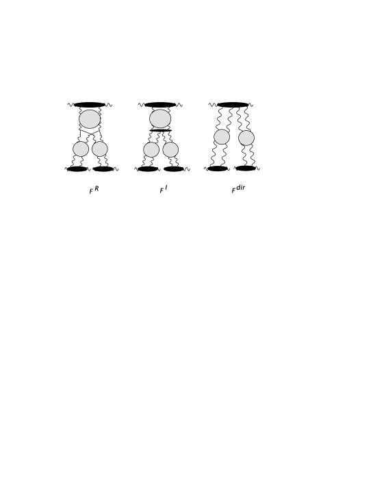
Figure 11: Large-$N_{c}$ limit of the six-point function

Compared to non-supersymmetric $\text{SU}(N_{c})$ gauge theories with fundamental quarks, the most striking difference is the presence of the last piece which exists only in the supersymmetric extension where all particles are in the adjoint representation. The triple Pomeron vertex, on the other hand, is the same in both cases. A detailed discussion of the topological expansion of the triple Pomeron vertex in the amplitudes above and its large-$N_{c}$ behavior has been given in [36, 62].

7 Summary and outlook

In this paper we have studied, in the generalized leading logarithmic approximation, the high energy behavior of ${\cal N}=4$ SYM in the triple Regge limit. It is this kinematic regime which, in QCD, exhibits the Möbius invariant triple Pomeron vertex. As the main result, we have found that in ${\cal N}=4$ SYM, with the fermions and scalars belonging to the adjoint representation of the gauge group $\text{SU}(N_{c})$, the four-gluon impact factor contains a novel piece whose existence can be traced back to the adjoint representation of the fermions and scalars. It has no counterpart in QCD where the quarks transform in the fundamental representation of the gauge group. In the six-point amplitude, this additional piece in the impact factor generates a coupling of the four-gluon state to the external currents which is absent in QCD. On the other hand, the triple Pomeron vertex in ${\cal N}=4$ SYM, in leading order, is the same as in the non-supersymmetric case. This supports the fundamental nature of this building block of Reggeon field theory: because of Regge factorization it has to be independent of the coupling to the external projectiles. In our case, this coupling is mediated by the impact factors in which the difference between ${\cal N}=4$ SYM and non-supersymmetric QCD is manifest: the fact that in both cases the triple Pomeron vertex is the same proves that factorization is indeed satisfied.

Appendix A Color algebra

In the calculations in section 3 and in appendix B we make use of the following $\text{SU}(N_{c})$ color identities,

$$f_{lak}f_{kbl} = {}-N_{c}\,\delta_{ab}\,,$$ (100)

$$f_{kal}f_{lbm}f_{mck} = {}-\frac{N_{c}}{2}\,f_{abc}\,,$$ (101)

$$f_{kal}f_{lbm}f_{mcn}f_{ndk} = {}N_{c}\,d^{abcd}+\frac{1}{2}(\delta_{ab}\delta_{cd}+\delta_{ac}\delta_{bd}+\delta_{ad}\delta_{bc})\,,$$ (102)

$$f_{kal}f_{lbm}f_{mcn}f_{ndo}f_{oek} = {}N_{c}\,f^{abcde}$$ (103)

$${}+\frac{1}{4}(\delta_{ab}f_{cde}+\delta_{ac}f_{bde}+\delta_{ad}f_{bce}+\delta_{ae}f_{bcd}$$

$${}\hskip 19.91684pt+f_{ade}\delta_{bc}+f_{ace}\delta_{bd}+f_{acd}\delta_{be}+f_{abe}\delta_{cd}$$

$${}\hskip 19.91684pt+f_{abd}\delta_{ce}+f_{abc}\delta_{de})\,,$$

where the tensors $d^{abcd}$ and $f^{abcde}$ are defined in (36) and (106), respectively. The first three identities are well-known while the last one has been derived in [9]. That paper also contains a description of a general and convenient way to obtain such identities using birdtrack notation.

It is worth pointing out that the relevant color tensors for the adjoint impact factors in the Pomeron channel satisfy

$$\mbox{tr}\,(T^{a_{1}}\dots T^{a_{n}})+(-1)^{n}\mbox{tr}\,(T^{a_{n}}\dots T^{a_{1}})=2\,\mbox{tr}\,(T^{a_{1}}\dots T^{a_{n}})\,.$$ (104)

We finally note that the $d$-tensor of (36) can be decomposed according to

$$d^{abcd}=\frac{1}{2N_{c}}\delta_{ab}\delta_{cd}+\frac{1}{4}(d_{abk}d_{kcd}-f_{abk}f_{kcd})\,.$$ (105)

Appendix B The five-gluon amplitude

In this appendix we would like to investigate the five-gluon amplitude in ${\cal N}=4$ SYM in the EGLLA. The main focus of this paper has been the four-gluon amplitude relevant for the six-point $R$-current correlator. The considerations in the present and in the following appendix C aim at a better understanding of the field theory structure of the amplitudes in the EGLLA. The main properties of that structure and its relation to reggeization have been described in section 5 for the case of the four-gluon amplitude. Here we want to discuss the five-gluon amplitude. We will show that, as a consequence of reggeization, it can be written completely in terms of elements of the 2-dimensional effective field theory which have been found already in the four-gluon amplitude.

Let us start with the five-gluon impact factor ${\mathchoice{\hbox{$\displaystyle\mathbb{D}$}}{\hbox{$\textstyle\mathbb{D}$}}{\hbox{$\scriptstyle\mathbb{D}$}}{\hbox{$\scriptscriptstyle\mathbb{D}$}}}_{(5;0)}$. I consists again of a fermionic and a scalar contribution. We follow the same steps as in section 3. In the case of five gluons the color tensors relevant for the impact factor in the fundamental representation (i. e. in QCD) are of the type

$$f^{abcde}=\frac{1}{i}[\mbox{tr}\,(t^{a}t^{b}t^{c}t^{d}t^{e})-\mbox{tr}\,(t^{e}t^{d}t^{c}t^{b}t^{a})]\,.$$ (106)

For the case of an impact factor consisting of a loop made of particles in the adjoint representation one obtains instead

$$\frac{1}{i}[\mbox{tr}\,(T^{a}T^{b}T^{c}T^{d}T^{e})-\mbox{tr}\,(T^{e}T^{d}T^{c}T^{b}T^{a})]$$ (107)

$$= {}2N_{c}f^{abcde}+\frac{1}{2}(\delta_{ab}f_{cde}+\delta_{ac}f_{bde}+\delta_{ad}f_{bce}+\delta_{ae}f_{bcd}+\delta_{bc}f_{ade}+\delta_{bd}f_{ace}$$

$${}\hskip 68.28644pt+\delta_{be}f_{acd}+\delta_{cd}f_{abe}+\delta_{ce}f_{abd}+\delta_{de}f_{abc})\,,$$

where we have used (103) and (104). Again, an additional color tensor structure occurs which was not present in the fundamental representation. For the fermionic contribution ${\mathchoice{\hbox{$\displaystyle\mathbb{D}$}}{\hbox{$\textstyle\mathbb{D}$}}{\hbox{$\scriptstyle\mathbb{D}$}}{\hbox{$\scriptscriptstyle\mathbb{D}$}}}_{F,(5;0)}$ to the impact factor this implies that we can decompose it into a part that is a multiple of the fundamental impact factor and an additional term as

$${\mathchoice{\hbox{$\displaystyle\mathbb{D}$}}{\hbox{$\textstyle\mathbb{D}$}}{\hbox{$\scriptstyle\mathbb{D}$}}{\hbox{$\scriptscriptstyle\mathbb{D}$}}}_{F,(5;0)}^{a_{1}a_{2}a_{3}a_{4}a_{5}}({\bf k}_{1},{\bf k}_{2},{\bf k}_{3},{\bf k}_{4},{\bf k}_{5})$$ (108)

$$= {}2N_{c}R\,D_{(5;0)}^{a_{1}a_{2}a_{3}a_{4}a_{5}}({\bf k}_{1},{\bf k}_{2},{\bf k}_{3},{\bf k}_{4},{\bf k}_{5})+{\mathchoice{\hbox{$\displaystyle\mathbb{D}$}}{\hbox{$\textstyle\mathbb{D}$}}{\hbox{$\scriptstyle\mathbb{D}$}}{\hbox{$\scriptscriptstyle\mathbb{D}$}}}_{F,(5;0)\,\text{dir}}^{a_{1}a_{2}a_{3}a_{4}a_{5}}({\bf k}_{1},{\bf k}_{2},{\bf k}_{3},{\bf k}_{4},{\bf k}_{5})\,.$$

With the help of the explicit expression for $D_{(5;0)}$ found in [9],

$$D_{(5;0)}^{a_{1}a_{2}a_{3}a_{4}a_{5}}({\bf k}_{1},{\bf k}_{2},{\bf k}_{3},{\bf k}_{4},{\bf k}_{5})$$

$$= {}-g^{3}\{f^{a_{1}a_{2}a_{3}a_{4}a_{5}}\,[D_{(2;0)}(1234,5)+D_{(2;0)}(1,2345)-D_{(2;0)}(15,234)]$$

$${}\,+f^{a_{2}a_{1}a_{3}a_{4}a_{5}}\,[D_{(2;0)}(1345,2)-D_{(2;0)}(12,345)+D_{(2;0)}(125,34)-D_{(2;0)}(134,25)]$$

$${}\,+f^{a_{1}a_{2}a_{3}a_{5}a_{4}}\,[D_{(2;0)}(1235,4)-D_{(2;0)}(14,235)+D_{(2;0)}(145,23)-D_{(2;0)}(123,45)]$$

$${}\,+f^{a_{1}a_{2}a_{4}a_{5}a_{3}}\,[D_{(2;0)}(1245,3)-D_{(2;0)}(13,245)+D_{(2;0)}(135,24)-D_{(2;0)}(124,35)]\}\,,$$

we can thus write

$${\mathchoice{\hbox{$\displaystyle\mathbb{D}$}}{\hbox{$\textstyle\mathbb{D}$}}{\hbox{$\scriptstyle\mathbb{D}$}}{\hbox{$\scriptscriptstyle\mathbb{D}$}}}_{F,(5;0)}^{a_{1}a_{2}a_{3}a_{4}a_{5}}({\bf k}_{1},{\bf k}_{2},{\bf k}_{3},{\bf k}_{4},{\bf k}_{5})$$ (110)

$$= {}-g^{3}\{f^{a_{1}a_{2}a_{3}a_{4}a_{5}}\,[{\mathchoice{\hbox{$\displaystyle\mathbb{D}$}}{\hbox{$\textstyle\mathbb{D}$}}{\hbox{$\scriptstyle\mathbb{D}$}}{\hbox{$\scriptscriptstyle\mathbb{D}$}}}_{F,(2;0)}(1234,5)+{\mathchoice{\hbox{$\displaystyle\mathbb{D}$}}{\hbox{$\textstyle\mathbb{D}$}}{\hbox{$\scriptstyle\mathbb{D}$}}{\hbox{$\scriptscriptstyle\mathbb{D}$}}}_{F(2;0)}(1,2345)-{\mathchoice{\hbox{$\displaystyle\mathbb{D}$}}{\hbox{$\textstyle\mathbb{D}$}}{\hbox{$\scriptstyle\mathbb{D}$}}{\hbox{$\scriptscriptstyle\mathbb{D}$}}}_{F,(2;0)}(15,234)]$$

$${}\,+f^{a_{2}a_{1}a_{3}a_{4}a_{5}}\,[{\mathchoice{\hbox{$\displaystyle\mathbb{D}$}}{\hbox{$\textstyle\mathbb{D}$}}{\hbox{$\scriptstyle\mathbb{D}$}}{\hbox{$\scriptscriptstyle\mathbb{D}$}}}_{F,(2;0)}(1345,2)-{\mathchoice{\hbox{$\displaystyle\mathbb{D}$}}{\hbox{$\textstyle\mathbb{D}$}}{\hbox{$\scriptstyle\mathbb{D}$}}{\hbox{$\scriptscriptstyle\mathbb{D}$}}}_{F,(2;0)}(12,345)+{\mathchoice{\hbox{$\displaystyle\mathbb{D}$}}{\hbox{$\textstyle\mathbb{D}$}}{\hbox{$\scriptstyle\mathbb{D}$}}{\hbox{$\scriptscriptstyle\mathbb{D}$}}}_{F,(2;0)}(125,34)-{\mathchoice{\hbox{$\displaystyle\mathbb{D}$}}{\hbox{$\textstyle\mathbb{D}$}}{\hbox{$\scriptstyle\mathbb{D}$}}{\hbox{$\scriptscriptstyle\mathbb{D}$}}}_{F,(2;0)}(134,25)]$$

$${}\,+f^{a_{1}a_{2}a_{3}a_{5}a_{4}}\,[{\mathchoice{\hbox{$\displaystyle\mathbb{D}$}}{\hbox{$\textstyle\mathbb{D}$}}{\hbox{$\scriptstyle\mathbb{D}$}}{\hbox{$\scriptscriptstyle\mathbb{D}$}}}_{F,(2;0)}(1235,4)-{\mathchoice{\hbox{$\displaystyle\mathbb{D}$}}{\hbox{$\textstyle\mathbb{D}$}}{\hbox{$\scriptstyle\mathbb{D}$}}{\hbox{$\scriptscriptstyle\mathbb{D}$}}}_{F,(2;0)}(14,235)+{\mathchoice{\hbox{$\displaystyle\mathbb{D}$}}{\hbox{$\textstyle\mathbb{D}$}}{\hbox{$\scriptstyle\mathbb{D}$}}{\hbox{$\scriptscriptstyle\mathbb{D}$}}}_{F,(2;0)}(145,23)-{\mathchoice{\hbox{$\displaystyle\mathbb{D}$}}{\hbox{$\textstyle\mathbb{D}$}}{\hbox{$\scriptstyle\mathbb{D}$}}{\hbox{$\scriptscriptstyle\mathbb{D}$}}}_{F,(2;0)}(123,45)]$$

$${}\,+f^{a_{1}a_{2}a_{4}a_{5}a_{3}}\,[{\mathchoice{\hbox{$\displaystyle\mathbb{D}$}}{\hbox{$\textstyle\mathbb{D}$}}{\hbox{$\scriptstyle\mathbb{D}$}}{\hbox{$\scriptscriptstyle\mathbb{D}$}}}_{F,(2;0)}(1245,3)-{\mathchoice{\hbox{$\displaystyle\mathbb{D}$}}{\hbox{$\textstyle\mathbb{D}$}}{\hbox{$\scriptstyle\mathbb{D}$}}{\hbox{$\scriptscriptstyle\mathbb{D}$}}}_{F,(2;0)}(13,245)+{\mathchoice{\hbox{$\displaystyle\mathbb{D}$}}{\hbox{$\textstyle\mathbb{D}$}}{\hbox{$\scriptstyle\mathbb{D}$}}{\hbox{$\scriptscriptstyle\mathbb{D}$}}}_{F,(2;0)}(135,24)-{\mathchoice{\hbox{$\displaystyle\mathbb{D}$}}{\hbox{$\textstyle\mathbb{D}$}}{\hbox{$\scriptstyle\mathbb{D}$}}{\hbox{$\scriptscriptstyle\mathbb{D}$}}}_{F,(2;0)}(124,35)]\}$$

$${}+{\mathchoice{\hbox{$\displaystyle\mathbb{D}$}}{\hbox{$\textstyle\mathbb{D}$}}{\hbox{$\scriptstyle\mathbb{D}$}}{\hbox{$\scriptscriptstyle\mathbb{D}$}}}_{F,(5;0)\,\text{dir}}^{a_{1}a_{2}a_{3}a_{4}a_{5}}({\bf k}_{1},{\bf k}_{2},{\bf k}_{3},{\bf k}_{4},{\bf k}_{5})\,$$

The additional piece, ${\mathchoice{\hbox{$\displaystyle\mathbb{D}$}}{\hbox{$\textstyle\mathbb{D}$}}{\hbox{$\scriptstyle\mathbb{D}$}}{\hbox{$\scriptscriptstyle\mathbb{D}$}}}_{F,(5;0)\,\text{dir}}$, is obtained explicitly by replacing the different tensors of type $f^{abcde}$ in eq. (B) by the additional color tensors emerging in eq. (107). A lengthy but straightforward calculation shows that the result can also be expressed in terms of the additional piece ${\mathchoice{\hbox{$\displaystyle\mathbb{D}$}}{\hbox{$\textstyle\mathbb{D}$}}{\hbox{$\scriptstyle\mathbb{D}$}}{\hbox{$\scriptscriptstyle\mathbb{D}$}}}_{(4;0)\;\text{dir}}$ found previously in the four-gluon amplitude (see eq. (39)) as

$${\mathchoice{\hbox{$\displaystyle\mathbb{D}$}}{\hbox{$\textstyle\mathbb{D}$}}{\hbox{$\scriptstyle\mathbb{D}$}}{\hbox{$\scriptscriptstyle\mathbb{D}$}}}^{a_{1}a_{2}a_{3}a_{4}a_{5}}_{F,(5;0)\,\text{dir}}({\bf k}_{1},{\bf k}_{2},{\bf k}_{3},{\bf k}_{4},{\bf k}_{5})$$ (111)

$$= {}\frac{g}{2}\left[f_{a_{1}a_{2}c}\,{\mathchoice{\hbox{$\displaystyle\mathbb{D}$}}{\hbox{$\textstyle\mathbb{D}$}}{\hbox{$\scriptstyle\mathbb{D}$}}{\hbox{$\scriptscriptstyle\mathbb{D}$}}}_{F,(4;0)\text{dir}}^{ca_{3}a_{4}a_{5}}(12,3,4,5)+f_{a_{1}a_{3}c}\,{\mathchoice{\hbox{$\displaystyle\mathbb{D}$}}{\hbox{$\textstyle\mathbb{D}$}}{\hbox{$\scriptstyle\mathbb{D}$}}{\hbox{$\scriptscriptstyle\mathbb{D}$}}}_{F,(4;0)\;\text{dir}}^{ca_{2}a_{4}a_{5}}(13,2,4,5)\right.$$

$${}\hskip 34.14322pt+\,f_{a_{1}a_{4}c}\,{\mathchoice{\hbox{$\displaystyle\mathbb{D}$}}{\hbox{$\textstyle\mathbb{D}$}}{\hbox{$\scriptstyle\mathbb{D}$}}{\hbox{$\scriptscriptstyle\mathbb{D}$}}}_{F,(4;0)\text{dir}}^{ca_{2}a_{3}a_{5}}(14,2,3,5)+f_{a_{1}a_{5}c}\,{\mathchoice{\hbox{$\displaystyle\mathbb{D}$}}{\hbox{$\textstyle\mathbb{D}$}}{\hbox{$\scriptstyle\mathbb{D}$}}{\hbox{$\scriptscriptstyle\mathbb{D}$}}}_{F,(4;0)\,\text{dir}}^{ca_{2}a_{3}a_{4}}(15,2,3,4)$$

$${}\hskip 34.14322pt+\,f_{a_{2}a_{3}c}\,{\mathchoice{\hbox{$\displaystyle\mathbb{D}$}}{\hbox{$\textstyle\mathbb{D}$}}{\hbox{$\scriptstyle\mathbb{D}$}}{\hbox{$\scriptscriptstyle\mathbb{D}$}}}_{F,(4;0)\,\text{dir}}^{a_{1}ca_{4}a_{5}}(1,23,4,5)+f_{a_{2}a_{4}c}\,{\mathchoice{\hbox{$\displaystyle\mathbb{D}$}}{\hbox{$\textstyle\mathbb{D}$}}{\hbox{$\scriptstyle\mathbb{D}$}}{\hbox{$\scriptscriptstyle\mathbb{D}$}}}_{F,(4;0)\,\text{dir}}^{a_{1}ca_{3}a_{5}}(1,24,3,5)$$

$${}\hskip 34.14322pt+\,f_{a_{2}a_{5}c}\,{\mathchoice{\hbox{$\displaystyle\mathbb{D}$}}{\hbox{$\textstyle\mathbb{D}$}}{\hbox{$\scriptstyle\mathbb{D}$}}{\hbox{$\scriptscriptstyle\mathbb{D}$}}}_{F,(4;0)\,\text{dir}}^{a_{1}ca_{3}a_{4}}(1,25,3,4)+f_{a_{3}a_{4}c}\,{\mathchoice{\hbox{$\displaystyle\mathbb{D}$}}{\hbox{$\textstyle\mathbb{D}$}}{\hbox{$\scriptstyle\mathbb{D}$}}{\hbox{$\scriptscriptstyle\mathbb{D}$}}}_{F,(4;0)\,\text{dir}}^{a_{1}a_{2}ca_{5}}(1,2,34,5)$$

$${}\hskip 34.14322pt\left.+\,f_{a_{3}a_{5}c}\,{\mathchoice{\hbox{$\displaystyle\mathbb{D}$}}{\hbox{$\textstyle\mathbb{D}$}}{\hbox{$\scriptstyle\mathbb{D}$}}{\hbox{$\scriptscriptstyle\mathbb{D}$}}}_{F,(4;0)\,\text{dir}}^{a_{1}a_{2}ca_{4}}(1,2,35,4)+f_{a_{4}a_{5}c}\,{\mathchoice{\hbox{$\displaystyle\mathbb{D}$}}{\hbox{$\textstyle\mathbb{D}$}}{\hbox{$\scriptstyle\mathbb{D}$}}{\hbox{$\scriptscriptstyle\mathbb{D}$}}}_{F,(4;0)\,\text{dir}}^{a_{1}a_{2}a_{3}c}(1,2,3,45)\right]\,.$$

It is straightforward to show that equations analogous to (110) and (111) are valid also for the scalar contribution ${\mathchoice{\hbox{$\displaystyle\mathbb{D}$}}{\hbox{$\textstyle\mathbb{D}$}}{\hbox{$\scriptstyle\mathbb{D}$}}{\hbox{$\scriptscriptstyle\mathbb{D}$}}}_{S,(5;0)}$ to the impact factor, that is also the additional piece ${\mathchoice{\hbox{$\displaystyle\mathbb{D}$}}{\hbox{$\textstyle\mathbb{D}$}}{\hbox{$\scriptstyle\mathbb{D}$}}{\hbox{$\scriptscriptstyle\mathbb{D}$}}}_{S,(5;0)\,\text{dir}}$ can be expressed in terms of the additional piece ${\mathchoice{\hbox{$\displaystyle\mathbb{D}$}}{\hbox{$\textstyle\mathbb{D}$}}{\hbox{$\scriptstyle\mathbb{D}$}}{\hbox{$\scriptscriptstyle\mathbb{D}$}}}_{S,(4;0)\,\text{dir}}$ of the four-gluon amplitude. Consequently, we obtain relations for the full impact factor ${\mathchoice{\hbox{$\displaystyle\mathbb{D}$}}{\hbox{$\textstyle\mathbb{D}$}}{\hbox{$\scriptstyle\mathbb{D}$}}{\hbox{$\scriptscriptstyle\mathbb{D}$}}}_{(5;0)}={\mathchoice{\hbox{$\displaystyle\mathbb{D}$}}{\hbox{$\textstyle\mathbb{D}$}}{\hbox{$\scriptstyle\mathbb{D}$}}{\hbox{$\scriptscriptstyle\mathbb{D}$}}}_{F,(5;0)}+{\mathchoice{\hbox{$\displaystyle\mathbb{D}$}}{\hbox{$\textstyle\mathbb{D}$}}{\hbox{$\scriptstyle\mathbb{D}$}}{\hbox{$\scriptscriptstyle\mathbb{D}$}}}_{S,(5;0)}$ which are completely analogous to (110) and (111). More precisely, eq. (110) and eq. (111) are valid after dropping the index $F$ in all terms. The second of these relations has been given explicitly for the full impact factor in eq. (49).

This representation shows that the additional piece ${\mathchoice{\hbox{$\displaystyle\mathbb{D}$}}{\hbox{$\textstyle\mathbb{D}$}}{\hbox{$\scriptstyle\mathbb{D}$}}{\hbox{$\scriptscriptstyle\mathbb{D}$}}}_{(5;0)\,\text{dir}}$ again exhibits reggeization. In each term in eq. (49) a pair of gluons in the color octet representation acts as a single gluon which enters the amplitude ${\mathchoice{\hbox{$\displaystyle\mathbb{D}$}}{\hbox{$\textstyle\mathbb{D}$}}{\hbox{$\scriptstyle\mathbb{D}$}}{\hbox{$\scriptscriptstyle\mathbb{D}$}}}_{(4;0)\,\text{dir}}$. In a certain sense this gluon can be regarded as a composite object of the two gluons merging into it. The full expression for ${\mathchoice{\hbox{$\displaystyle\mathbb{D}$}}{\hbox{$\textstyle\mathbb{D}$}}{\hbox{$\scriptstyle\mathbb{D}$}}{\hbox{$\scriptscriptstyle\mathbb{D}$}}}_{(5;0)\,\text{dir}}$ is then obtained by summing over all possible pairs of gluons. We recall that the amplitude ${\mathchoice{\hbox{$\displaystyle\mathbb{D}$}}{\hbox{$\textstyle\mathbb{D}$}}{\hbox{$\scriptstyle\mathbb{D}$}}{\hbox{$\scriptscriptstyle\mathbb{D}$}}}_{(4;0)\,\text{dir}}$ is fully symmetric in its momentum and color arguments such that it is not relevant at which position the more composite gluon formed from the pair is inserted in ${\mathchoice{\hbox{$\displaystyle\mathbb{D}$}}{\hbox{$\textstyle\mathbb{D}$}}{\hbox{$\scriptstyle\mathbb{D}$}}{\hbox{$\scriptscriptstyle\mathbb{D}$}}}_{(4;0)\,\text{dir}}$.

We can now put the picture derived form the three- and four-gluon amplitudes to the test by considering the integral equation for the five-gluon amplitude. According to the expected field theory structure we should find that the five-gluon amplitude ${\mathchoice{\hbox{$\displaystyle\mathbb{D}$}}{\hbox{$\textstyle\mathbb{D}$}}{\hbox{$\scriptstyle\mathbb{D}$}}{\hbox{$\scriptscriptstyle\mathbb{D}$}}}_{5}$ reggeizes, that means it should be possible to express it completely in terms of elements that are already present in the lower amplitudes. This should now in particular include ${\mathchoice{\hbox{$\displaystyle\mathbb{D}$}}{\hbox{$\textstyle\mathbb{D}$}}{\hbox{$\scriptstyle\mathbb{D}$}}{\hbox{$\scriptscriptstyle\mathbb{D}$}}}_{(4;0)\,\text{dir}}$ which we have identified as a new element of our field theory. The evolution equation for ${\mathchoice{\hbox{$\displaystyle\mathbb{D}$}}{\hbox{$\textstyle\mathbb{D}$}}{\hbox{$\scriptstyle\mathbb{D}$}}{\hbox{$\scriptscriptstyle\mathbb{D}$}}}_{5}^{a_{1}a_{2}a_{3}a_{4}a_{5}}$ reads

$$\left(\omega-\sum_{i=1}^{5}\beta({\bf k}_{i})\right){\mathchoice{\hbox{$\displaystyle\mathbb{D}$}}{\hbox{$\textstyle\mathbb{D}$}}{\hbox{$\scriptstyle\mathbb{D}$}}{\hbox{$\scriptscriptstyle\mathbb{D}$}}}_{5}^{a_{1}a_{2}a_{3}a_{4}a_{5}} = {}{\mathchoice{\hbox{$\displaystyle\mathbb{D}$}}{\hbox{$\textstyle\mathbb{D}$}}{\hbox{$\scriptstyle\mathbb{D}$}}{\hbox{$\scriptscriptstyle\mathbb{D}$}}}_{(5;0)}^{a_{1}a_{2}a_{3}a_{4}a_{5}}+K^{\{b\}\rightarrow\{a\}}_{2\rightarrow 5}\otimes{\mathchoice{\hbox{$\displaystyle\mathbb{D}$}}{\hbox{$\textstyle\mathbb{D}$}}{\hbox{$\scriptstyle\mathbb{D}$}}{\hbox{$\scriptscriptstyle\mathbb{D}$}}}_{2}^{b_{1}b_{2}}$$ (112)

$${}+\sum K^{\{b\}\rightarrow\{a\}}_{2\rightarrow 4}\otimes{\mathchoice{\hbox{$\displaystyle\mathbb{D}$}}{\hbox{$\textstyle\mathbb{D}$}}{\hbox{$\scriptstyle\mathbb{D}$}}{\hbox{$\scriptscriptstyle\mathbb{D}$}}}_{3}^{b_{1}b_{2}b_{3}}+\sum K^{\{b\}\rightarrow\{a\}}_{2\rightarrow 3}\otimes{\mathchoice{\hbox{$\displaystyle\mathbb{D}$}}{\hbox{$\textstyle\mathbb{D}$}}{\hbox{$\scriptstyle\mathbb{D}$}}{\hbox{$\scriptscriptstyle\mathbb{D}$}}}_{4}^{b_{1}b_{2}b_{3}b_{4}}$$

$${}+\sum K^{\{b\}\rightarrow\{a\}}_{2\rightarrow 2}\otimes{\mathchoice{\hbox{$\displaystyle\mathbb{D}$}}{\hbox{$\textstyle\mathbb{D}$}}{\hbox{$\scriptstyle\mathbb{D}$}}{\hbox{$\scriptscriptstyle\mathbb{D}$}}}_{5}^{b_{1}b_{2}b_{3}b_{4}b_{5}}\,,$$

which can be graphically illustrated as

$$\left(\omega-\sum_{i=1}^{5}\beta({\bf k}_{i})\right)\hbox{\raise-16.06749pt\hbox{\includegraphics{glD51}}} = {}\hbox{\raise-14.1767pt\hbox{\includegraphics{glD52}}}+\hbox{\raise-16.06749pt\hbox{\includegraphics{glD53}}}+\sum\hbox{\raise-16.06749pt\hbox{\includegraphics{glD54}}}$$ (113)

$${}+\sum\hbox{\raise-16.06749pt\hbox{\includegraphics{glD55}}}+\sum\hbox{\raise-16.06749pt\hbox{\includegraphics{glD56}}}\,.$$

In view of the results found for the amplitudes with up to four gluons, and since the adjoint impact factor with five gluons (108) consists of a multiple of the fundamental impact factor and a new (additional) piece, it is natural to decompose the full amplitude ${\mathchoice{\hbox{$\displaystyle\mathbb{D}$}}{\hbox{$\textstyle\mathbb{D}$}}{\hbox{$\scriptstyle\mathbb{D}$}}{\hbox{$\scriptscriptstyle\mathbb{D}$}}}_{5}$ according to

$${\mathchoice{\hbox{$\displaystyle\mathbb{D}$}}{\hbox{$\textstyle\mathbb{D}$}}{\hbox{$\scriptstyle\mathbb{D}$}}{\hbox{$\scriptscriptstyle\mathbb{D}$}}}_{5}={\mathchoice{\hbox{$\displaystyle\mathbb{D}$}}{\hbox{$\textstyle\mathbb{D}$}}{\hbox{$\scriptstyle\mathbb{D}$}}{\hbox{$\scriptscriptstyle\mathbb{D}$}}}_{5}^{R}+{\mathchoice{\hbox{$\displaystyle\mathbb{D}$}}{\hbox{$\textstyle\mathbb{D}$}}{\hbox{$\scriptstyle\mathbb{D}$}}{\hbox{$\scriptscriptstyle\mathbb{D}$}}}_{5}^{I}+{\mathchoice{\hbox{$\displaystyle\mathbb{D}$}}{\hbox{$\textstyle\mathbb{D}$}}{\hbox{$\scriptstyle\mathbb{D}$}}{\hbox{$\scriptscriptstyle\mathbb{D}$}}}_{5\,\text{dir}}\,,$$ (114)

where the first two parts are multiples of the corresponding amplitudes $D_{5}^{R}$ and $D_{5}^{I}$ known from QCD with fundamental quarks. There, these two parts exhaust the full amplitude, whereas here we will have an additional part ${\mathchoice{\hbox{$\displaystyle\mathbb{D}$}}{\hbox{$\textstyle\mathbb{D}$}}{\hbox{$\scriptstyle\mathbb{D}$}}{\hbox{$\scriptscriptstyle\mathbb{D}$}}}_{5\,\text{dir}}$. According to this picture we find, using the results of [9],

$${\mathchoice{\hbox{$\displaystyle\mathbb{D}$}}{\hbox{$\textstyle\mathbb{D}$}}{\hbox{$\scriptstyle\mathbb{D}$}}{\hbox{$\scriptscriptstyle\mathbb{D}$}}}_{5}^{R\,a_{1}a_{2}a_{3}a_{4}a_{5}}({\bf k}_{1},{\bf k}_{2},{\bf k}_{3},{\bf k}_{4},{\bf k}_{5})=$$

$$= {}-g^{3}\{f^{a_{1}a_{2}a_{3}a_{4}a_{5}}\,[{\mathchoice{\hbox{$\displaystyle\mathbb{D}$}}{\hbox{$\textstyle\mathbb{D}$}}{\hbox{$\scriptstyle\mathbb{D}$}}{\hbox{$\scriptscriptstyle\mathbb{D}$}}}_{2}(1234,5)+{\mathchoice{\hbox{$\displaystyle\mathbb{D}$}}{\hbox{$\textstyle\mathbb{D}$}}{\hbox{$\scriptstyle\mathbb{D}$}}{\hbox{$\scriptscriptstyle\mathbb{D}$}}}_{2}(1,2345)-{\mathchoice{\hbox{$\displaystyle\mathbb{D}$}}{\hbox{$\textstyle\mathbb{D}$}}{\hbox{$\scriptstyle\mathbb{D}$}}{\hbox{$\scriptscriptstyle\mathbb{D}$}}}_{2}(15,234)]$$

$${}\phantom{-g^{3}}+f^{a_{2}a_{1}a_{3}a_{4}a_{5}}\,[{\mathchoice{\hbox{$\displaystyle\mathbb{D}$}}{\hbox{$\textstyle\mathbb{D}$}}{\hbox{$\scriptstyle\mathbb{D}$}}{\hbox{$\scriptscriptstyle\mathbb{D}$}}}_{2}(1345,2)-{\mathchoice{\hbox{$\displaystyle\mathbb{D}$}}{\hbox{$\textstyle\mathbb{D}$}}{\hbox{$\scriptstyle\mathbb{D}$}}{\hbox{$\scriptscriptstyle\mathbb{D}$}}}_{2}(12,345)+{\mathchoice{\hbox{$\displaystyle\mathbb{D}$}}{\hbox{$\textstyle\mathbb{D}$}}{\hbox{$\scriptstyle\mathbb{D}$}}{\hbox{$\scriptscriptstyle\mathbb{D}$}}}_{2}(125,34)-{\mathchoice{\hbox{$\displaystyle\mathbb{D}$}}{\hbox{$\textstyle\mathbb{D}$}}{\hbox{$\scriptstyle\mathbb{D}$}}{\hbox{$\scriptscriptstyle\mathbb{D}$}}}_{2}(134,25)]$$

$${}\phantom{-g^{3}}+f^{a_{1}a_{2}a_{3}a_{5}a_{4}}\,[{\mathchoice{\hbox{$\displaystyle\mathbb{D}$}}{\hbox{$\textstyle\mathbb{D}$}}{\hbox{$\scriptstyle\mathbb{D}$}}{\hbox{$\scriptscriptstyle\mathbb{D}$}}}_{2}(1235,4)-{\mathchoice{\hbox{$\displaystyle\mathbb{D}$}}{\hbox{$\textstyle\mathbb{D}$}}{\hbox{$\scriptstyle\mathbb{D}$}}{\hbox{$\scriptscriptstyle\mathbb{D}$}}}_{2}(14,235)+{\mathchoice{\hbox{$\displaystyle\mathbb{D}$}}{\hbox{$\textstyle\mathbb{D}$}}{\hbox{$\scriptstyle\mathbb{D}$}}{\hbox{$\scriptscriptstyle\mathbb{D}$}}}_{2}(145,23)-{\mathchoice{\hbox{$\displaystyle\mathbb{D}$}}{\hbox{$\textstyle\mathbb{D}$}}{\hbox{$\scriptstyle\mathbb{D}$}}{\hbox{$\scriptscriptstyle\mathbb{D}$}}}_{2}(123,45)]$$

$${}\phantom{-g^{3}}+f^{a_{1}a_{2}a_{4}a_{5}a_{3}}\,[{\mathchoice{\hbox{$\displaystyle\mathbb{D}$}}{\hbox{$\textstyle\mathbb{D}$}}{\hbox{$\scriptstyle\mathbb{D}$}}{\hbox{$\scriptscriptstyle\mathbb{D}$}}}_{2}(1245,3)-{\mathchoice{\hbox{$\displaystyle\mathbb{D}$}}{\hbox{$\textstyle\mathbb{D}$}}{\hbox{$\scriptstyle\mathbb{D}$}}{\hbox{$\scriptscriptstyle\mathbb{D}$}}}_{2}(13,245)+{\mathchoice{\hbox{$\displaystyle\mathbb{D}$}}{\hbox{$\textstyle\mathbb{D}$}}{\hbox{$\scriptstyle\mathbb{D}$}}{\hbox{$\scriptscriptstyle\mathbb{D}$}}}_{2}(135,24)-{\mathchoice{\hbox{$\displaystyle\mathbb{D}$}}{\hbox{$\textstyle\mathbb{D}$}}{\hbox{$\scriptstyle\mathbb{D}$}}{\hbox{$\scriptscriptstyle\mathbb{D}$}}}_{2}(124,35)]\}$$

and

$${\mathchoice{\hbox{$\displaystyle\mathbb{D}$}}{\hbox{$\textstyle\mathbb{D}$}}{\hbox{$\scriptstyle\mathbb{D}$}}{\hbox{$\scriptscriptstyle\mathbb{D}$}}}_{5}^{I\,a_{1}a_{2}a_{3}a_{4}a_{5}}({\bf k}_{1},{\bf k}_{2},{\bf k}_{3},{\bf k}_{4},{\bf k}_{5})$$ (116)

$${}=\frac{g}{2}\left\{f_{a_{1}a_{2}c}{\mathchoice{\hbox{$\displaystyle\mathbb{D}$}}{\hbox{$\textstyle\mathbb{D}$}}{\hbox{$\scriptstyle\mathbb{D}$}}{\hbox{$\scriptscriptstyle\mathbb{D}$}}}_{4}^{I\,ca_{3}a_{4}a_{5}}(12,3,4,5)+f_{a_{1}a_{3}c}{\mathchoice{\hbox{$\displaystyle\mathbb{D}$}}{\hbox{$\textstyle\mathbb{D}$}}{\hbox{$\scriptstyle\mathbb{D}$}}{\hbox{$\scriptscriptstyle\mathbb{D}$}}}_{4}^{I\,ca_{2}a_{4}a_{5}}(13,2,4,5)\right.$$

$${}\hskip 14.22636pt+\,f_{a_{1}a_{4}c}{\mathchoice{\hbox{$\displaystyle\mathbb{D}$}}{\hbox{$\textstyle\mathbb{D}$}}{\hbox{$\scriptstyle\mathbb{D}$}}{\hbox{$\scriptscriptstyle\mathbb{D}$}}}_{4}^{I\,ca_{2}a_{3}a_{5}}(14,2,3,5)+f_{a_{1}a_{5}c}{\mathchoice{\hbox{$\displaystyle\mathbb{D}$}}{\hbox{$\textstyle\mathbb{D}$}}{\hbox{$\scriptstyle\mathbb{D}$}}{\hbox{$\scriptscriptstyle\mathbb{D}$}}}_{4}^{I\,ca_{2}a_{3}a_{4}}(15,2,3,4)$$

$${}\hskip 14.22636pt+\,f_{a_{2}a_{3}c}{\mathchoice{\hbox{$\displaystyle\mathbb{D}$}}{\hbox{$\textstyle\mathbb{D}$}}{\hbox{$\scriptstyle\mathbb{D}$}}{\hbox{$\scriptscriptstyle\mathbb{D}$}}}_{4}^{I\,a_{1}ca_{4}a_{5}}(1,23,4,5)+f_{a_{2}a_{4}c}{\mathchoice{\hbox{$\displaystyle\mathbb{D}$}}{\hbox{$\textstyle\mathbb{D}$}}{\hbox{$\scriptstyle\mathbb{D}$}}{\hbox{$\scriptscriptstyle\mathbb{D}$}}}_{4}^{I\,a_{1}ca_{3}a_{5}}(1,24,3,5)$$

$${}\hskip 14.22636pt+\,f_{a_{2}a_{5}c}{\mathchoice{\hbox{$\displaystyle\mathbb{D}$}}{\hbox{$\textstyle\mathbb{D}$}}{\hbox{$\scriptstyle\mathbb{D}$}}{\hbox{$\scriptscriptstyle\mathbb{D}$}}}_{4}^{I\,a_{1}ca_{3}a_{4}}(1,25,3,4)+f_{a_{3}a_{4}c}{\mathchoice{\hbox{$\displaystyle\mathbb{D}$}}{\hbox{$\textstyle\mathbb{D}$}}{\hbox{$\scriptstyle\mathbb{D}$}}{\hbox{$\scriptscriptstyle\mathbb{D}$}}}_{4}^{I\,a_{1}a_{2}ca_{5}}(1,2,34,5)$$

$${}\hskip 14.22636pt\left.+\,f_{a_{3}a_{5}c}{\mathchoice{\hbox{$\displaystyle\mathbb{D}$}}{\hbox{$\textstyle\mathbb{D}$}}{\hbox{$\scriptstyle\mathbb{D}$}}{\hbox{$\scriptscriptstyle\mathbb{D}$}}}_{4}^{I\,a_{1}a_{2}ca_{4}}(1,2,35,4)+f_{a_{4}a_{5}c}{\mathchoice{\hbox{$\displaystyle\mathbb{D}$}}{\hbox{$\textstyle\mathbb{D}$}}{\hbox{$\scriptstyle\mathbb{D}$}}{\hbox{$\scriptscriptstyle\mathbb{D}$}}}_{4}^{I\,a_{1}a_{2}a_{3}c}(1,2,3,45)\right\}\,.$$

We have directly written these two parts in terms of the adjoint amplitudes ${\mathchoice{\hbox{$\displaystyle\mathbb{D}$}}{\hbox{$\textstyle\mathbb{D}$}}{\hbox{$\scriptstyle\mathbb{D}$}}{\hbox{$\scriptscriptstyle\mathbb{D}$}}}_{2}$. For the fermionic part we have in particular ${\mathchoice{\hbox{$\displaystyle\mathbb{D}$}}{\hbox{$\textstyle\mathbb{D}$}}{\hbox{$\scriptstyle\mathbb{D}$}}{\hbox{$\scriptscriptstyle\mathbb{D}$}}}_{F,5}^{R}=2N_{c}RD_{5}^{R}$ and ${\mathchoice{\hbox{$\displaystyle\mathbb{D}$}}{\hbox{$\textstyle\mathbb{D}$}}{\hbox{$\scriptstyle\mathbb{D}$}}{\hbox{$\scriptscriptstyle\mathbb{D}$}}}_{F,5}^{I}=2N_{c}RD_{5}^{I}$. Inserting then eq. (114) into the integral equation (112) and invoking the integral equation for $D_{5}$ treated in [9] we obtain a new integral equation for the additional part ${\mathchoice{\hbox{$\displaystyle\mathbb{D}$}}{\hbox{$\textstyle\mathbb{D}$}}{\hbox{$\scriptstyle\mathbb{D}$}}{\hbox{$\scriptscriptstyle\mathbb{D}$}}}_{5\,\text{dir}}$,

$$\left(\omega-\sum_{i=1}^{5}\beta({\bf k}_{i})\right){\mathchoice{\hbox{$\displaystyle\mathbb{D}$}}{\hbox{$\textstyle\mathbb{D}$}}{\hbox{$\scriptstyle\mathbb{D}$}}{\hbox{$\scriptscriptstyle\mathbb{D}$}}}_{5\,\text{dir}}^{a_{1}a_{2}a_{3}a_{4}a_{5}} = {}{\mathchoice{\hbox{$\displaystyle\mathbb{D}$}}{\hbox{$\textstyle\mathbb{D}$}}{\hbox{$\scriptstyle\mathbb{D}$}}{\hbox{$\scriptscriptstyle\mathbb{D}$}}}_{(5;0)\,\text{dir}}^{a_{1}a_{2}a_{3}a_{4}a_{5}}+\sum K^{\{b\}\rightarrow\{a\}}_{2\rightarrow 3}\otimes{\mathchoice{\hbox{$\displaystyle\mathbb{D}$}}{\hbox{$\textstyle\mathbb{D}$}}{\hbox{$\scriptstyle\mathbb{D}$}}{\hbox{$\scriptscriptstyle\mathbb{D}$}}}_{4\,\text{dir}}^{b_{1}b_{2}b_{3}b_{4}}$$ (117)

$${}+\sum K^{\{b\}\rightarrow\{a\}}_{2\rightarrow 2}\otimes{\mathchoice{\hbox{$\displaystyle\mathbb{D}$}}{\hbox{$\textstyle\mathbb{D}$}}{\hbox{$\scriptstyle\mathbb{D}$}}{\hbox{$\scriptscriptstyle\mathbb{D}$}}}_{5\,\text{dir}}^{b_{1}b_{2}b_{3}b_{4}b_{5}}\,.$$

We recall that the inhomogeneous term ${\mathchoice{\hbox{$\displaystyle\mathbb{D}$}}{\hbox{$\textstyle\mathbb{D}$}}{\hbox{$\scriptstyle\mathbb{D}$}}{\hbox{$\scriptscriptstyle\mathbb{D}$}}}_{(5;0)\,\text{dir}}$ reggeizes and is a superposition of amplitudes ${\mathchoice{\hbox{$\displaystyle\mathbb{D}$}}{\hbox{$\textstyle\mathbb{D}$}}{\hbox{$\scriptstyle\mathbb{D}$}}{\hbox{$\scriptscriptstyle\mathbb{D}$}}}_{(4;0)\,\text{dir}}$ of the form (49). Therefore the structure of this equation coincides with that of the integral equations for ${\mathchoice{\hbox{$\displaystyle\mathbb{D}$}}{\hbox{$\textstyle\mathbb{D}$}}{\hbox{$\scriptstyle\mathbb{D}$}}{\hbox{$\scriptscriptstyle\mathbb{D}$}}}_{3}$ and $D_{5}^{I}$. It can be solved employing a known identity involving the integral kernels $K_{2\to 2}$ and $K_{2\to 3}$. In terms of the diagrams of (63) this identity can be written as

$$\hbox{\raise-283.1892pt\hbox{\includegraphics{reggel1}}}+\hbox{\raise-283.1892pt\hbox{\includegraphics{reggel2}}}+\hbox{\raise-283.1892pt\hbox{\includegraphics{reggel3}}} = \frac{2}{g}\,\hbox{\raise-283.1892pt\hbox{\includegraphics{regger1}}}+\hbox{\raise-283.1892pt\hbox{\includegraphics{regger2}}}+\hbox{\raise-283.1892pt\hbox{\includegraphics{regger3}}}$$ (118)

$$+\hbox{\raise-283.1892pt\hbox{\includegraphics{regger4}}}+\hbox{\raise-283.1892pt\hbox{\includegraphics{regger5}}}+\hbox{\raise-283.1892pt\hbox{\includegraphics{regger6}}}+\hbox{\raise-283.1892pt\hbox{\includegraphics{regger7}}}\,,$$

where the unaffected gluons are not drawn. The vertices in which two lines merge into one, drawn here with a small full dot, indicate that the two lower gluons merge into the upper one with a color factor $f_{abc}$ and in such a way that their transverse momenta are added. The arrows on the top of the diagrams indicate that the identity holds for gluons in amplitudes that are symmetric under the exchange of this pair of gluons (or symmetric under the exchange of any pair of gluons). This is the case for the amplitude ${\mathchoice{\hbox{$\displaystyle\mathbb{D}$}}{\hbox{$\textstyle\mathbb{D}$}}{\hbox{$\scriptstyle\mathbb{D}$}}{\hbox{$\scriptscriptstyle\mathbb{D}$}}}_{4\,\text{dir}}$ as we have discussed above. For a more detailed description of the application of the identity (118) to completely analogous situations we refer the reader to [9] or [41]. In this way one finds the solution of eq. (117) to have the form

$${\mathchoice{\hbox{$\displaystyle\mathbb{D}$}}{\hbox{$\textstyle\mathbb{D}$}}{\hbox{$\scriptstyle\mathbb{D}$}}{\hbox{$\scriptscriptstyle\mathbb{D}$}}}_{5\,\text{dir}}^{a_{1}a_{2}a_{3}a_{4}a_{5}}({\bf k}_{1},{\bf k}_{2},{\bf k}_{3},{\bf k}_{4},{\bf k}_{5})$$ (119)

$${}=\frac{g}{2}\left\{f_{a_{1}a_{2}c}{\mathchoice{\hbox{$\displaystyle\mathbb{D}$}}{\hbox{$\textstyle\mathbb{D}$}}{\hbox{$\scriptstyle\mathbb{D}$}}{\hbox{$\scriptscriptstyle\mathbb{D}$}}}_{4\,\text{dir}}^{ca_{3}a_{4}a_{5}}(12,3,4,5)+f_{a_{1}a_{3}c}{\mathchoice{\hbox{$\displaystyle\mathbb{D}$}}{\hbox{$\textstyle\mathbb{D}$}}{\hbox{$\scriptstyle\mathbb{D}$}}{\hbox{$\scriptscriptstyle\mathbb{D}$}}}_{4\,\text{dir}}^{ca_{2}a_{4}a_{5}}(13,2,4,5)\right.$$

$${}\hskip 14.22636pt+\,f_{a_{1}a_{4}c}{\mathchoice{\hbox{$\displaystyle\mathbb{D}$}}{\hbox{$\textstyle\mathbb{D}$}}{\hbox{$\scriptstyle\mathbb{D}$}}{\hbox{$\scriptscriptstyle\mathbb{D}$}}}_{4\,\text{dir}}^{ca_{2}a_{3}a_{5}}(14,2,3,5)+f_{a_{1}a_{5}c}{\mathchoice{\hbox{$\displaystyle\mathbb{D}$}}{\hbox{$\textstyle\mathbb{D}$}}{\hbox{$\scriptstyle\mathbb{D}$}}{\hbox{$\scriptscriptstyle\mathbb{D}$}}}_{4\,\text{dir}}^{ca_{2}a_{3}a_{4}}(15,2,3,4)$$

$${}\hskip 14.22636pt+\,f_{a_{2}a_{3}c}{\mathchoice{\hbox{$\displaystyle\mathbb{D}$}}{\hbox{$\textstyle\mathbb{D}$}}{\hbox{$\scriptstyle\mathbb{D}$}}{\hbox{$\scriptscriptstyle\mathbb{D}$}}}_{4\,\text{dir}}^{a_{1}ca_{4}a_{5}}(1,23,4,5)+f_{a_{2}a_{4}c}{\mathchoice{\hbox{$\displaystyle\mathbb{D}$}}{\hbox{$\textstyle\mathbb{D}$}}{\hbox{$\scriptstyle\mathbb{D}$}}{\hbox{$\scriptscriptstyle\mathbb{D}$}}}_{4\,\text{dir}}^{a_{1}ca_{3}a_{5}}(1,24,3,5)$$

$${}\hskip 14.22636pt+\,f_{a_{2}a_{5}c}{\mathchoice{\hbox{$\displaystyle\mathbb{D}$}}{\hbox{$\textstyle\mathbb{D}$}}{\hbox{$\scriptstyle\mathbb{D}$}}{\hbox{$\scriptscriptstyle\mathbb{D}$}}}_{4\,\text{dir}}^{a_{1}ca_{3}a_{4}}(1,25,3,4)+f_{a_{3}a_{4}c}{\mathchoice{\hbox{$\displaystyle\mathbb{D}$}}{\hbox{$\textstyle\mathbb{D}$}}{\hbox{$\scriptstyle\mathbb{D}$}}{\hbox{$\scriptscriptstyle\mathbb{D}$}}}_{4\,\text{dir}}^{a_{1}a_{2}ca_{5}}(1,2,34,5)$$

$${}\hskip 14.22636pt\left.+\,f_{a_{3}a_{5}c}{\mathchoice{\hbox{$\displaystyle\mathbb{D}$}}{\hbox{$\textstyle\mathbb{D}$}}{\hbox{$\scriptstyle\mathbb{D}$}}{\hbox{$\scriptscriptstyle\mathbb{D}$}}}_{4\,\text{dir}}^{a_{1}a_{2}ca_{4}}(1,2,35,4)+f_{a_{4}a_{5}c}{\mathchoice{\hbox{$\displaystyle\mathbb{D}$}}{\hbox{$\textstyle\mathbb{D}$}}{\hbox{$\scriptstyle\mathbb{D}$}}{\hbox{$\scriptscriptstyle\mathbb{D}$}}}_{4\,\text{dir}}^{a_{1}a_{2}a_{3}c}(1,2,3,45)\right\}\,.$$

One immediately recognizes that this amplitudes again exhibits reggeization. It is a superposition of the four-gluon amplitudes ${\mathchoice{\hbox{$\displaystyle\mathbb{D}$}}{\hbox{$\textstyle\mathbb{D}$}}{\hbox{$\scriptstyle\mathbb{D}$}}{\hbox{$\scriptscriptstyle\mathbb{D}$}}}_{4\,\text{dir}}$, and in each term of the superposition two gluons in a color octet combine to form a more composite reggeized gluon that enters the amplitude ${\mathchoice{\hbox{$\displaystyle\mathbb{D}$}}{\hbox{$\textstyle\mathbb{D}$}}{\hbox{$\scriptstyle\mathbb{D}$}}{\hbox{$\scriptscriptstyle\mathbb{D}$}}}_{4\,\text{dir}}$. The sum over all possible pairs of this kind gives the additional part of the full five-gluon amplitude ${\mathchoice{\hbox{$\displaystyle\mathbb{D}$}}{\hbox{$\textstyle\mathbb{D}$}}{\hbox{$\scriptstyle\mathbb{D}$}}{\hbox{$\scriptscriptstyle\mathbb{D}$}}}_{5}$. One can easily check from eq. (119) that this expression satisfies the Ward-type identities of [56], and hence all parts of the amplitude ${\mathchoice{\hbox{$\displaystyle\mathbb{D}$}}{\hbox{$\textstyle\mathbb{D}$}}{\hbox{$\scriptstyle\mathbb{D}$}}{\hbox{$\scriptscriptstyle\mathbb{D}$}}}_{5}$ share that property.

In summary, we have solved the integral equation (112) for the five-gluon amplitude ${\mathchoice{\hbox{$\displaystyle\mathbb{D}$}}{\hbox{$\textstyle\mathbb{D}$}}{\hbox{$\scriptstyle\mathbb{D}$}}{\hbox{$\scriptscriptstyle\mathbb{D}$}}}_{5}$ and have expressed the solution in terms of the lower amplitudes ${\mathchoice{\hbox{$\displaystyle\mathbb{D}$}}{\hbox{$\textstyle\mathbb{D}$}}{\hbox{$\scriptstyle\mathbb{D}$}}{\hbox{$\scriptscriptstyle\mathbb{D}$}}}_{2}$, ${\mathchoice{\hbox{$\displaystyle\mathbb{D}$}}{\hbox{$\textstyle\mathbb{D}$}}{\hbox{$\scriptstyle\mathbb{D}$}}{\hbox{$\scriptscriptstyle\mathbb{D}$}}}_{4}^{I}$ and ${\mathchoice{\hbox{$\displaystyle\mathbb{D}$}}{\hbox{$\textstyle\mathbb{D}$}}{\hbox{$\scriptstyle\mathbb{D}$}}{\hbox{$\scriptscriptstyle\mathbb{D}$}}}_{4\,\text{dir}}$. Diagrammatically, the solution has the form

$${\mathchoice{\hbox{$\displaystyle\mathbb{D}$}}{\hbox{$\textstyle\mathbb{D}$}}{\hbox{$\scriptstyle\mathbb{D}$}}{\hbox{$\scriptscriptstyle\mathbb{D}$}}}_{5}=\sum\hbox{\raise-36.66444pt\hbox{\includegraphics[width=51.21504pt]{Db51}}}+\sum\hbox{\raise-51.11844pt\hbox{\includegraphics[width=56.9055pt]{Db52}}}+\sum\hbox{\raise-33.05095pt\hbox{\includegraphics[width=65.44142pt]{Db53}}}\,.$$ (120)

The first two terms are multiples of the amplitudes known from the case of QCD with fundamental quarks. The last terms is an additional term that exhibits exactly the features expected from the picture of the effective field theory structure discussed above, in particular it reggeizes exactly as expected and fulfills the Ward-type identities of [56]. Hence we find that the five-gluon amplitude precisely meets our expectations based on that underlying picture.

Appendix C Some remarks on the six-gluon amplitude

In this appendix we want to consider some aspects of the six-gluon amplitude ${\mathchoice{\hbox{$\displaystyle\mathbb{D}$}}{\hbox{$\textstyle\mathbb{D}$}}{\hbox{$\scriptstyle\mathbb{D}$}}{\hbox{$\scriptscriptstyle\mathbb{D}$}}}_{6}$ in the EGLLA for ${\cal N}=$ SYM. Our motivation is that it would obviously be interesting to see whether and how the field theory structure found above in the amplitudes ${\mathchoice{\hbox{$\displaystyle\mathbb{D}$}}{\hbox{$\textstyle\mathbb{D}$}}{\hbox{$\scriptstyle\mathbb{D}$}}{\hbox{$\scriptscriptstyle\mathbb{D}$}}}_{n}$ for$n\leq 5$ continues in the amplitudes with more than five gluons. Already in QCD with fundamental quarks the six-gluon amplitude involves some additional complication, see the discussion in [9]. A full analysis of the six-gluon is beyond the scope of the present paper and is left for future work. It might be particularly interesting to find out whether another new element of the effective field theory emerges that would couple six gluons directly to the adjoint quark loop – in analogy to the element ${\mathchoice{\hbox{$\displaystyle\mathbb{D}$}}{\hbox{$\textstyle\mathbb{D}$}}{\hbox{$\scriptstyle\mathbb{D}$}}{\hbox{$\scriptscriptstyle\mathbb{D}$}}}_{(4;0)\,\text{add}}$ with four gluons found above. From the results obtained here the picture emerges that in general (that is for arbitrary $n$) the amplitudes ${\mathchoice{\hbox{$\displaystyle\mathbb{D}$}}{\hbox{$\textstyle\mathbb{D}$}}{\hbox{$\scriptstyle\mathbb{D}$}}{\hbox{$\scriptscriptstyle\mathbb{D}$}}}_{n}$ always contain a multiple of the amplitudes $D_{n}$ with fundamental quarks plus additional new terms. Those latter contain on the one hand terms originating from the scalar contribution to the impact factor, and their structure concerning reggeization is very similar to that observed in the terms coming from the fermionic impact factor. On the other hand, there are new terms, for example the one coupling four gluons directly to the impact factor.

Although we do not make an attempt here to solve the whole six-gluon amplitude we can rather easily make an interesting observation concerning ${\mathchoice{\hbox{$\displaystyle\mathbb{D}$}}{\hbox{$\textstyle\mathbb{D}$}}{\hbox{$\scriptstyle\mathbb{D}$}}{\hbox{$\scriptscriptstyle\mathbb{D}$}}}_{6}$ which in fact confirms that expectation. Namely, one finds that similarly to the case of the lower amplitudes the terms known from the corresponding amplitude $D_{6}$ of QCD with fundamental fermions are reproduced (again up to a normalization factor) together with their scalar counterparts, and additional terms are generated. In particular, the same transition from two to six gluons via the vertex $V_{2\to 6}$ computed in [9] (containing both a coupling of a Pomeron to two Odderons and a transition from one to three Pomerons) occurs again in the amplitude ${\mathchoice{\hbox{$\displaystyle\mathbb{D}$}}{\hbox{$\textstyle\mathbb{D}$}}{\hbox{$\scriptstyle\mathbb{D}$}}{\hbox{$\scriptscriptstyle\mathbb{D}$}}}_{6}$.

The diagrams with six gluons coupling to the fermion or scalar loop give rise to a color tensor of the type

$$\mbox{tr}\,(T^{a}T^{b}T^{c}T^{d}T^{e}T^{f})+\mbox{tr}\,(T^{f}T^{e}T^{d}T^{c}T^{b}T^{a}) = {}2\,\mbox{tr}\,(T^{a}T^{b}T^{c}T^{d}T^{e}T^{f})$$ (121)

$$= {}-2f_{kal}f_{lbm}f_{mcn}f_{ndo}f_{oep}f_{pfk}$$

instead of the tensor

$$d^{abcdef}=\mbox{tr}\,(t^{a}t^{b}t^{c}t^{d}t^{e}t^{f})+\mbox{tr}\,(t^{f}t^{e}t^{d}t^{c}t^{b}t^{a})$$ (122)

obtained for quarks in the fundamental representation. We can therefore obtain the adjoint fermion impact factor ${\mathchoice{\hbox{$\displaystyle\mathbb{D}$}}{\hbox{$\textstyle\mathbb{D}$}}{\hbox{$\scriptstyle\mathbb{D}$}}{\hbox{$\scriptscriptstyle\mathbb{D}$}}}_{F,(6;0)}$ from the known expression for the fundamental impact factor $D_{(6;0)}$ (see [9]), by replacing the color tensors of type (122) in this expression by the corresponding color tensors of type (121), besides decorating it with the usual factor $R$ accounting for the different numbers of fermionic degrees of freedom running around the loop. But now one has [9]

$$f_{kal}f_{lbm}f_{mcn}f_{ndo}f_{oep}f_{pfk} = {}-N_{c}d^{abcdef}$$ (123)

$${}-\frac{1}{2}(\delta_{ab}d^{cdef}+\delta_{ac}d^{bdef}+\delta_{ad}d^{bcef}+\delta_{ae}d^{bcdf}$$

$${}\hskip 19.91684pt+\delta_{af}d^{bcde}+d^{adef}\delta_{bc}+d^{acef}\delta_{bd}+d^{acdf}\delta_{be}$$

$${}\hskip 19.91684pt+d^{acde}\delta_{bf}+d^{abef}\delta_{cd}+d^{abdf}\delta_{ce}+d^{abde}\delta_{cf}$$

$${}\hskip 19.91684pt+d^{abcf}\delta_{de}+d^{abce}\delta_{df}+d^{abcd}\delta_{ef})$$

$${}+\frac{1}{8}[(d_{abc}d_{def}+f_{abc}f_{def})+(d_{abd}d_{cef}+f_{abd}f_{cef})$$

$${}\hskip 19.91684pt+(d_{abe}d_{cdf}+f_{abe}f_{cdf})+(d_{abf}d_{cde}+f_{abf}f_{cde})$$

$${}\hskip 19.91684pt+(d_{acd}d_{bef}+f_{acd}f_{bef})+(d_{ace}d_{bdf}+f_{ace}f_{bdf})$$

$${}\hskip 19.91684pt+(d_{acf}d_{bde}+f_{acf}f_{bde})+(d_{ade}d_{bcf}+f_{ade}f_{bcf})$$

$${}\hskip 19.91684pt+(d_{adf}d_{bce}+f_{adf}f_{bce})+(d_{aef}d_{bcd}+f_{aef}f_{bcd})]$$

$$= {}-N_{c}d^{abcdef}+\Theta^{abcdef}\,,$$ (124)

where the last equation defines the tensor $\Theta^{abcdef}$. Therefore inserting the color tensors of type (121) one naturally obtains two contributions to the fermion impact factor ${\mathchoice{\hbox{$\displaystyle\mathbb{D}$}}{\hbox{$\textstyle\mathbb{D}$}}{\hbox{$\scriptstyle\mathbb{D}$}}{\hbox{$\scriptscriptstyle\mathbb{D}$}}}_{F,(6;0)}$,

$${\mathchoice{\hbox{$\displaystyle\mathbb{D}$}}{\hbox{$\textstyle\mathbb{D}$}}{\hbox{$\scriptstyle\mathbb{D}$}}{\hbox{$\scriptscriptstyle\mathbb{D}$}}}_{F,(6;0)}^{a_{1}a_{2}a_{3}a_{4}a_{5}a_{6}}({\bf k}_{1},{\bf k}_{2},{\bf k}_{3},{\bf k}_{4},{\bf k}_{5},{\bf k}_{6}) = {}2N_{c}RD_{(6;0)}^{a_{1}a_{2}a_{3}a_{4}a_{5}a_{6}}({\bf k}_{1},{\bf k}_{2},{\bf k}_{3},{\bf k}_{4},{\bf k}_{5},{\bf k}_{6})$$ (125)

$${}+{\mathchoice{\hbox{$\displaystyle\mathbb{D}$}}{\hbox{$\textstyle\mathbb{D}$}}{\hbox{$\scriptstyle\mathbb{D}$}}{\hbox{$\scriptscriptstyle\mathbb{D}$}}}^{a_{1}a_{2}a_{3}a_{4}a_{5}a_{6}}_{(6;0)\,\text{dir}}({\bf k}_{1},{\bf k}_{2},{\bf k}_{3},{\bf k}_{4},{\bf k}_{5},{\bf k}_{6})\,$$

where

$$D_{(6;0)}^{a_{1}a_{2}a_{3}a_{4}a_{5}a_{6}}({\bf k}_{1},{\bf k}_{2},{\bf k}_{3},{\bf k}_{4},{\bf k}_{5},{\bf k}_{6})=$$ (126)

$$= g^{4}\{d^{a_{1}a_{2}a_{3}a_{4}a_{5}a_{6}}\,[D_{(2;0)}(12345,6)+D_{(2;0)}(1,23456)-D_{(2;0)}(16,2345)]$$

$$\,+\,d^{a_{2}a_{1}a_{3}a_{4}a_{5}a_{6}}\,[D_{(2;0)}(13456,2)-D_{(2;0)}(1345,26)+D_{(2;0)}(126,345)$$

$$\hskip 85.35826pt-D_{(2;0)}(12,3456)]$$

$$\,+\,d^{a_{1}a_{2}a_{3}a_{4}a_{6}a_{5}}\,[D_{(2;0)}(12346,5)-D_{(2;0)}(1234,56)+D_{(2;0)}(156,234)$$

$$\hskip 85.35826pt-D_{(2;0)}(15,2346)]$$

$$\,+\,d^{a_{2}a_{1}a_{3}a_{4}a_{6}a_{5}}\,[-D_{(2;0)}(1256,34)-D_{(2;0)}(1346,25)+D_{(2;0)}(125,346)$$

$$\hskip 85.35826pt+D_{(2;0)}(134,256)]$$

$$\,+\,d^{a_{3}a_{1}a_{2}a_{4}a_{5}a_{6}}\,[D_{(2;0)}(12456,3)-D_{(2;0)}(1245,36)+D_{(2;0)}(136,245)$$

$$\hskip 85.35826pt-D_{(2;0)}(13,2456)]$$

$$\,+\,d^{a_{1}a_{2}a_{3}a_{5}a_{6}a_{4}}\,[D_{(2;0)}(12356,4)-D_{(2;0)}(1235,46)+D_{(2;0)}(146,235)$$

$$\hskip 85.35826pt-D_{(2;0)}(14,2356)]$$

$$\,+\,d^{a_{2}a_{1}a_{3}a_{5}a_{6}a_{4}}\,[-D_{(2;0)}(1246,35)-D_{(2;0)}(1356,24)+D_{(2;0)}(124,356)$$

$$\hskip 85.35826pt+D_{(2;0)}(135,246)]$$

$$\,+\,d^{a_{1}a_{2}a_{3}a_{6}a_{5}a_{4}}\,[-D_{(2;0)}(1236,45)-D_{(2;0)}(1456,23)+D_{(2;0)}(123,456)$$

$$\hskip 85.35826pt+D_{(2;0)}(145,236)]\}$$

Consequently, the first term on the r.h.s. of eq. (125) can again be expressed as a sum of two-gluon impact factors ${\mathchoice{\hbox{$\displaystyle\mathbb{D}$}}{\hbox{$\textstyle\mathbb{D}$}}{\hbox{$\scriptstyle\mathbb{D}$}}{\hbox{$\scriptscriptstyle\mathbb{D}$}}}_{F,(2;0)}=2N_{c}RD_{(2;0)}$. A similar expression can be obtained for the scalar impact factor ${\mathchoice{\hbox{$\displaystyle\mathbb{D}$}}{\hbox{$\textstyle\mathbb{D}$}}{\hbox{$\scriptstyle\mathbb{D}$}}{\hbox{$\scriptscriptstyle\mathbb{D}$}}}_{S,(6;0)}$.

The first contribution in eq. (125), arising from the first term in the decomposition eq. (124) of the adjoint color tensors, is just a multiple of the known six-gluon impact factor in the fundamental representation. The second contribution arises from the $\Theta$-tensors in (124) (as defined in (123) when inserting (121) for the $d$-tensors in (126)). It would be straightforward to write out the new additional term explicitly. As we have pointed out before it would be interesting to study in detail its relation to the new element ${\mathchoice{\hbox{$\displaystyle\mathbb{D}$}}{\hbox{$\textstyle\mathbb{D}$}}{\hbox{$\scriptstyle\mathbb{D}$}}{\hbox{$\scriptscriptstyle\mathbb{D}$}}}_{F,(4;0)\,\text{dir}}$ found there. This, however, is beyond the scope of the present paper. Here we restrict ourselves to the important finding that also the adjoint impact factor with six gluons is similar to those with four and five gluons: it reproduces as one of its contributions a multiple of the fundamental impact factor and in addition contains a new part that occurs only if the fermions are taken in the adjoint representation. A similar additional contribution is obtained from the adjoint scalars in the impact factor.

Inserting this result for ${\mathchoice{\hbox{$\displaystyle\mathbb{D}$}}{\hbox{$\textstyle\mathbb{D}$}}{\hbox{$\scriptstyle\mathbb{D}$}}{\hbox{$\scriptscriptstyle\mathbb{D}$}}}_{F,(6;0)\,\text{dir}}$ (and the analogous scalar part) in the integral equation for the full amplitude ${\mathchoice{\hbox{$\displaystyle\mathbb{D}$}}{\hbox{$\textstyle\mathbb{D}$}}{\hbox{$\scriptstyle\mathbb{D}$}}{\hbox{$\scriptscriptstyle\mathbb{D}$}}}_{6}$ we easily recognize that also the full amplitude consists of two parts, one of which is a multiple of the full six-gluon amplitude $D_{6}$ with fundamental quarks (together with its scalar counterpart) and hence inherits the conformal field theory structure found in that amplitude. In particular, this part contains exactly the same transition vertex from two to six gluons found in [9]. The structure of the other part remains to be investigated.

References

- [1] E. A. Kuraev, L. N. Lipatov and V. S. Fadin, Sov. Phys. JETP 45 (1977) 199 [Zh. Eksp. Teor. Fiz. 72 (1977) 377].
- [2] I. I. Balitsky and L. N. Lipatov, Sov. J. Nucl. Phys. 28 (1978) 822 [Yad. Fiz. 28 (1978) 1597].
- [3] V. N. Gribov, Sov. Phys. JETP 26 (1968) 414 [Zh. Eksp. Teor. Fiz. 53 (1967) 654].
- [4] J. Bartels, Nucl. Phys. B 175 (1980) 365.
- [5] J. Kwieciński and M. Praszałowicz, Phys. Lett. B 94 (1980) 413.
- [6] J. Bartels, Phys. Lett. B 298 (1993) 204.
- [7] J. Bartels, Z. Phys. C 60 (1993) 471.
- [8] J. Bartels and M. Wüsthoff, Z. Phys. C 66 (1995) 157.
- [9] J. Bartels and C. Ewerz, JHEP 9909 (1999) 026 [arXiv:hep-ph/9908454].
- [10] L. N. Lipatov, Nucl. Phys. B 365 (1991) 614.
- [11] L. N. Lipatov, Nucl. Phys. B 452 (1995) 369 [arXiv:hep-ph/9502308].
- [12] M. Hentschinski, arXiv:0908.2576 [hep-ph].
- [13] I. Balitsky, Nucl. Phys. B 463 (1996) 99 [arXiv:hep-ph/9509348].
- [14] I. Balitsky, Phys. Rev. D 60 (1999) 014020 [arXiv:hep-ph/9812311].
- [15] I. Balitsky, Phys. Lett. B 518 (2001) 235 [arXiv:hep-ph/0105334].
- [16] I. I. Balitsky and A. V. Belitsky, Nucl. Phys. B 629 (2002) 290 [arXiv:hep-ph/0110158].
- [17] A. H. Mueller, Nucl. Phys. B 415 (1994) 373.
- [18] A. H. Mueller and B. Patel, Nucl. Phys. B 425 (1994) 471 [arXiv:hep-ph/9403256].
- [19] A. H. Mueller, Nucl. Phys. B 437 (1995) 107 [arXiv:hep-ph/9408245].
- [20] Z. Chen and A. H. Mueller, Nucl. Phys. B 451 (1995) 579.
- [21] E. Iancu and R. Venugopalan, in Quark-Gluon Plasma 3, Eds. R. C. Hwa and X.-N. Wang, World Scientific (2003), arXiv:hep-ph/0303204.
- [22] Y. V. Kovchegov, Phys. Rev. D 54, 5463 (1996) [arXiv:hep-ph/9605446].
- [23] Y. V. Kovchegov, Phys. Rev. D 55, 5445 (1997) [arXiv:hep-ph/9701229].
- [24] L. N. Lipatov, Sov. Phys. JETP 63 (1986) 904 [Zh. Eksp. Teor. Fiz. 90 (1986) 1536].
- [25] J. Bartels, L. N. Lipatov and M. Wüsthoff, Nucl. Phys. B 464 (1996) 298 [arXiv:hep-ph/9509303].
- [26] C. Ewerz, Phys. Lett. B 512 (2001) 239 [arXiv:hep-ph/0105181].
- [27] L. N. Lipatov, arXiv:hep-th/9311037.
- [28] L. N. Lipatov, JETP Lett. 59 (1994) 596 [Pisma Zh. Eksp. Teor. Fiz. 59 (1994) 571].
- [29] L. D. Faddeev and G. P. Korchemsky, Phys. Lett. B 342 (1995) 311 [arXiv:hep-th/9404173].
- [30] J. M. Maldacena, Adv. Theor. Math. Phys. 2 (1998) 231 [Int. J. Theor. Phys. 38 (1999) 1113] [arXiv:hep-th/9711200].
- [31] S. S. Gubser, I. R. Klebanov and A. M. Polyakov, Phys. Lett. B 428 (1998) 105 [arXiv:hep-th/9802109].
- [32] E. Witten, Adv. Theor. Math. Phys. 2 (1998) 253 [arXiv:hep-th/9802150].
- [33] S. Caron-Huot, P. Kovtun, G. D. Moore, A. Starinets and L. G. Yaffe, JHEP 0612 (2006) 015 [arXiv:hep-th/0607237].
- [34] J. Bartels, A.-M. Mischler and M. Salvadore, Phys. Rev. D 78 (2008) 016004 [arXiv:0803.1423 [hep-ph]].
- [35] J. Bartels, J. Kotanski, A.-M. Mischler and V. Schomerus, arXiv:0908.2301 [hep-th].
- [36] J. Bartels, M. Hentschinski and A.-M. Mischler, Phys. Lett. B 679 (2009) 460 [arXiv:0906.3640 [hep-ph]].
- [37] R. C. Brower, C. E. DeTar and J. H. Weis, Phys. Rept. 14 (1974) 257.
- [38] L. Brink, J. H. Schwarz and J. Scherk, Nucl. Phys. B 121 (1977) 77.
- [39] L. Cornalba, M. S. Costa and J. Penedones, JHEP 0806 (2008) 048 [arXiv:0801.3002 [hep-th]].
- [40] L. Cornalba, M. S. Costa and J. Penedones, arXiv:0911.0043 [hep-th].
- [41] S. Braunewell and C. Ewerz, Nucl. Phys. A 760 (2005) 141 [arXiv:hep-ph/0501110].
- [42] C. Ewerz, arXiv:hep-ph/0306137.
- [43] R. C. Brower, M. Djuric and C. I. Tan, JHEP 0907 (2009) 063 [arXiv:0812.0354 [hep-th]].
- [44] L. N. Lipatov, Phys. Rept. 286 (1997) 131 [arXiv:hep-ph/9610276].
- [45] V. S. Fadin and L. N. Lipatov, Phys. Lett. B 429 (1998) 127 [arXiv:hep-ph/9802290].
- [46] M. Ciafaloni and G. Camici, Phys. Lett. B 430 (1998) 349 [arXiv:hep-ph/9803389].
- [47] A. V. Kotikov and L. N. Lipatov, Nucl. Phys. B 582 (2000) 19 [arXiv:hep-ph/0004008].
- [48] A. V. Kotikov and L. N. Lipatov, Nucl. Phys. B 661 (2003) 19 [Erratum-ibid. B 685 (2004) 405] [arXiv:hep-ph/0208220].
- [49] J. Bartels, DESY 91-074 (unpublished)
- [50] H. Lotter, Ph. D. Thesis, Hamburg University 1996, arXiv:hep-ph/9705288.
- [51] M. A. Braun and G. P. Vacca, Eur. Phys. J. C 6 (1999) 147 [arXiv:hep-ph/9711486].
- [52] M. Braun, Eur. Phys. J. C 6 (1999) 321 [arXiv:hep-ph/9706373].
- [53] G. P. Korchemsky, Nucl. Phys. B 550 (1999) 397 [arXiv:hep-ph/9711277].
- [54] C. Ewerz, Phys. Lett. B 472 (2000) 135 [arXiv:hep-ph/9911225].
- [55] G. P. Vacca, Phys. Lett. B 489 (2000) 337 [arXiv:hep-ph/0007067].
- [56] C. Ewerz, JHEP 0104 (2001) 031 [arXiv:hep-ph/0103260].
- [57] V. Schatz, Ph. D. Thesis, Heidelberg University 2003, arXiv:hep-ph/0307326.
- [58] C. Ewerz and V. Schatz, Nucl. Phys. A 736 (2004) 371 [arXiv:hep-ph/0308056].
- [59] J. Bartels, L. N. Lipatov and G. P. Vacca, Nucl. Phys. B 706 (2005) 391 [arXiv:hep-ph/0404110].
- [60] T. Bittig and C. Ewerz, Nucl. Phys. A 755 (2005) 616 [arXiv:hep-ph/0501192].
- [61] J. Bartels, M. Salvadore and G. P. Vacca, JHEP 0806 (2008) 032 [arXiv:0802.2702 [hep-ph]].
- [62] J. Bartels and M. Hentschinski, JHEP 0908 (2009) 103 [arXiv:0903.5464 [hep-ph]].
- [63] J. Bartels, J. Kotanski, A.-M. Mischler and V. Schomerus, arXiv:0912.3072 [hep-th].