Minimal Supersymmetric Hybrid Inflation, Flipped SU(5) and Proton Decay
Abstract
Minimal supersymmetric hybrid inflation utilizes a canonical Kähler potential and a renormalizable superpotential which is uniquely determined by imposing a U(1) -symmetry. In computing the scalar spectral index we take into account modifications of the tree level potential caused by radiative and supergravity corrections, as well as contributions from the soft supersymmetry breaking terms with a negative soft mass-squared term allowed for the inflaton. All of these contributions play a role in realizing values in the range 0.96–0.97 preferred by WMAP. The U(1) -symmetry plays an important role in flipped SU(5) by eliminating the troublesome dimension five proton decay. The proton decays into via dimension six operators arising from the exchange of superheavy gauge bosons with a lifetime of order – years.
Introduction
The past year has seen the successful launch of two exciting experimental efforts that promise to usher in a new era of high energy physics. On the ground, the Large Hadron Collider (LHC) at CERN will soon be scouring the TeV energy range, diligently seeking to confirm or deny a vast number of predictions. In the sky, the Planck Surveyor has taken up residence at the L2 Lagrange point, and is actively taking precise measurements of the Cosmic Microwave Background (CMB) to further elucidate the first moments of the universe’s existence. In high energy theory, establishing a robust and testable link between cosmology and mainstream particle physics remains an ongoing challenge. Models of supersymmetric (SUSY) hybrid inflation [1, 2, 3] involving low-scale ( TeV) SUSY and minimal () supergravity (SUGRA) [4] are particularly attractive in this sense, providing a natural connection between these two realms [5]. As a general feature, these models incorporate the spontaneous breaking of a SUSY gauge theory to its subgroup at the end of inflation (minimal hybrid inflation) or during inflation (shifted hybrid inflation [6]). In the simplest model [1], the CMB temperature anisotropy turns out to be on the order of , where is the symmetry breaking scale of . Then, in order for self-consistency of the inflationary scenario to be preserved, is comparable to the scale of grand unification, GeV, hinting that may constitute a grand unified theory (GUT). Two examples of that are highly motivated via their successes in mainstream particle physics include and the so-called flipped SU(5) model [7], SU(5)U(1)X; we will study the latter in great detail.
The flipped SU(5) model comprises a particularly suitable choice of , due to its many attractive features as a GUT model [8], as well as its connections to F-theory [9, 10]. In addition to lacking topological defects, flipped SU(5) also offers a natural resolution to the doublet-triplet splitting problem. The presence of a U(1) -symmetry suppresses the dimension five operators leading to proton decay. Proton decay via dimension six couplings to superheavy gauge bosons can still occur, and may lead to proton lifetimes within reach of upcoming experiments. In the context of inflation, -symmetry also leads to a unique renormalizable superpotential, thus flipped SU(5) constitutes an exceedingly natural choice of .
In addition to their connection with symmetry breaking, these hybrid inflationary models exhibit a number of other attractive features. For a wide range of parameters, the inflaton field amplitude takes on values that do not drastically exceed , in contrast with the trans-Planckian values obtained in the chaotic inflationary scenario. As a result, supergravity corrections remain under control in these models [11, 12]. In addition, it has been shown within the context of these models that one of the soft SUSY-breaking terms can play a significant role during inflation [12]. This same term has also been seen to play an integral role in resolving the MSSM problem [13]. Furthermore, it was recently shown [14] that inclusion of this soft term in the inflationary potential can lead to a reduced value of the scalar spectral index . SUSY hybrid inflation models that include only SUGRA and radiative corrections involve a well-known lower bound of , whereas the addition of a (negative) linear soft term can result in better agreement with the central value measured by the WMAP 5 yr analysis (WMAP5). The WMAP5 best estimate of the spectral index is given in Ref. [15] as . In the models treated here, however, the tensor-to-scalar ratio is exceedingly small (); thus we will use the estimate inferred from Ref. [15] for . (Accordingly, we will refer to the value as the ‘central value’ of WMAP5, pertaining to models of this type.) In this letter, we carefully investigate the role during inflation of a second soft SUSY-breaking term which modifies the mass of the inflaton field. Similarly to the study performed in Ref. [14], we find that its inclusion in the inflationary potential gives rise to a scalar spectral index which is in enhanced agreement with the WMAP5 central value. It is important to note that this result is achieved by employing the canonical (minimal) Kähler potential, the use of which also leads to the amelioration of the so-called ‘ problem.’ For other approaches to reducing the spectral index, including use of a non-minimal Kähler potential, see Refs. [16, 17, 18]. (For a recent study leading to the reduction of the spectral index in non-SUSY hybrid inflation, see Ref. [19].)
Minimal SUSY Hybrid Inflation
SUSY hybrid inflation models are described by the superpotential [1, 2]
| (1) |
where is a gauge singlet superfield acting as the inflaton, and , are conjugate superfields transforming nontrivially under some gauge group , and provide the vacuum energy associated with inflation. If one assumes an additional U(1)R ‘-symmetry,’ it can readily be seen that in Eq. (1) is the unique superpotential involving these superfields that is invariant under both U(1)R and at the renormalizable level.
The canonical Kähler potential may be written as
| (2) |
Recent analyses have used a non-minimal Kähler potential to obtain better agreement with WMAP5 (see, for example, Refs. [16, 17]). However, as we will see, the minimal Kähler potential will be sufficient for our purposes. The SUGRA scalar potential is given by
| (3) |
where represent the bosonic components of the superfields, , and where we have defined
and GeV is the reduced Planck mass. In the D-flat direction, ; then, using Eqs. (1)–(3), we may write the tree level global SUSY potential as
| (4) |
A suitable choice of initial conditions ensures that the fields become trapped in the (flat) valley along , . The gauge group is unbroken along this valley; however, only the constant term is present at tree level, thus SUSY is broken during inflation. Taking into account leading order SUGRA corrections, as well as radiative corrections [1] and soft SUSY-breaking terms, the flat valley is lifted and the inflaton rolls toward smaller values. Upon reaching its critical value , inflation ends via waterfall as the fields rapidly transition to the global SUSY minimum located at , , beginning damped oscillations about this vacuum to reheat the universe.
By including the various correction terms, we may write the scalar potential along the inflationary trajectory (i.e. ) as
| (5) |
where
| (6) |
represents radiative corrections, and
| (7) |
Here, parametrizes the inflaton field, is the dimensionality of the representation of fields and with respect to , TeV is the gravitino mass, and is the renormalization scale. The last two terms in Eq. (5) arise as soft SUSY-breaking linear and mass-squared terms, respectively, and their form here is derived from a gravity-mediated SUSY-breaking scheme [13]. The coupling is the coefficient of the linear soft term in the Lagrangian [20], and is expected. As can be seen from Eq. (7), the dimensionless parameter can have any sign; indeed, in a recent analysis [14], we have pointed out that choosing the negative sign can result in good agreement with the central value of the spectral index as measured by WMAP5 [15]. In the case of TeV-scale soft masses, this holds as long as with a magnitude . In our calculations, we will consider three representative examples, , . Note that a constant value of corresponds to negligible variation of , which can be achieved by employing an appropriate choice of initial condition [17].
In this letter, we investigate the effect of a negative soft mass-squared term for the inflaton (i.e. ) occurring at intermediate scales. The physical inflaton mass is given by
| (8) |
and so it is necessary that be significantly smaller than the tree-level mass in order to ensure that remains real. In our numerical calculations, this condition is met throughout the range of interest without needing to impose the restriction by hand. Tachyonic soft masses have previously been utilized to reduce fine tuning in the MSSM [21]. As we will see, a negative soft mass-squared term can produce a reduction of the spectral index similar to the case of , treated in Ref. [14], for a range of intermediate mass scales depending in part upon the sign of . The soft mass scales employed here are reminiscent in magnitude of split SUSY models, in which the scalar superpartners attain masses at a separate (typically much larger) scale compared to their fermionic counterparts [22]. A crucial difference between our models and split SUSY is the sign of the soft mass-squared term, which is positive in split SUSY.
The number of e-foldings after a given comoving scale has crossed the horizon is given by
| (9) |
where and denote the values of at and at the end of inflation, respectively. Inflation may end via a waterfall induced at if the slow-roll approximation holds. However, the slow-roll conditions are typically violated at slightly larger than unity, in which case inflation ends via slow-roll breakdown somewhat before the waterfall would occur. The number of e-folds after the scale corresponding to the WMAP pivot scale Mpc-1 exits the horizon is approximately given by
| (10) |
where we have assumed a matter-dominated reheating phase. The reheat temperature depends on the mechanism by which the universe was reheated after the end of inflation. As we do not wish to assume a specific reheating mechanism, we will use a constant value GeV, although lower values of may also be considered.
In Eq. (10) and throughout, a subscript ‘0’ denotes quantities taken at the pivot scale . In particular, the amplitude of the primordial curvature perturbation is given by
| (11) |
and has been measured by WMAP5 to be at [15]. This important constraint is useful in the determination of the value at the start of observable inflation.
In the case of , the potential in Eq. (5) monotonically increases with . In contrast, if either (or both) of these parameters is negative, a metastable (SUSY-broken) vacuum may be induced in some region of parameter space. However, it is possible to obtain enough e-foldings for successful inflation even if the local potential maximum occurs very close to . In our calculations, we will assume that the inflaton has successfully escaped any metastable vacua, and the solutions presented will correspond to the last 50–60 or so e-foldings occurring in a region where the potential monotonically increases with . When a metastable vacuum is present in the potential, inflation begins near the local maximum where the potential is concave downward, constituting ‘hilltop’ inflation [23]. This behavior is also exhibited in many cases in which the potential possesses points of inflection but lacks additional extrema.
The usual slow-roll parameters are given by
| (12) |
Within the framework of the slow-roll approximation (i.e. ), the scalar spectral index appears as
| (13) |
to leading order in the slow-roll parameters. (In our numerical calculations, we have used the next-to-leading order expressions in the slow-roll parameters for and other quantities, for additional precision.) The slow-roll parameter is quite small in these models, and is consistently subdominant in comparison to . Thus we have suppressed the contribution of the term in Eq. (13). The terms arising from radiative corrections and the soft mass-squared term both yield a negative contribution to , encouraging a red-tilted spectrum. (Notice that leads to an enhancement rather than reduction of the spectral index, and such a term pushes farther from the WMAP5 central value.) In addition, a subtle contribution from the soft linear term can play a significant role in determining the behavior of , arising indirectly via the WMAP5 normalization of and the shift of with a change of [14].
Flipped SU(5)
There are a number of natural choices for the gauge group . As mentioned previously, can be associated with a U(1)B-L symmetry, a case which is motivated in terms of generating the observed baryon asymmetry via leptogenesis. We may alternatively identify with a GUT, such as SO(10) or SU(5) [24]. An attractive choice is the so-called flipped SU(5) model, SU(5)U(1)X, which possesses a number of advantages over other models. In this case, symmetry breaking is induced by a 10-plet, i.e. and , and the superpotential is given by [8]
where denote the Yukawa couplings for quarks and charged leptons. (For a discussion of neutrino masses in these models, see Ref. [8].) The first line in Eq. (Flipped SU(5)) is relevant for inflation, and corresponds to the superpotential in Eq. (1). The terms in the second line are involved in the solution of the doublet-triplet splitting problem, and the last line contains terms that generate masses for quarks and charged leptons. Following [8], the charges of the multiplets with respect to the U(1)R -symmetry are assigned as
| (15) |
Note that U(1)R forbids the appearance of the bilinear term proportional to in the superpotential [8]. The color Higgs triplets in and become superheavy due to the couplings and , while the MSSM Higgs doublets remain light. Furthermore, the absence of the term in Eq. (Flipped SU(5)) leads to the dimension-five proton decay amplitude being heavily suppressed (by an additional factor , where TeV is the MSSM term). The problem can be solved, as previously discussed in Ref. [8], by exploiting the Giudice-Masiero mechanism [25]. Proton decay proceeds via the dimension-six operator, ()222For a recent discussion of proton decay in the context of non-SUSY inflation models, see Ref. [26].. (For further discussion of proton decay in the context of flipped SU(5), see Ref. [27].) Interestingly, it is the same U(1)R symmetry that we have already seen to be important for SUSY hybrid inflation that also alleviates some of the typical GUT problems.
The flipped SU(5) model exhibits yet more desirable features. In contrast to the U(1)B-L model, flipped SU(5) benefits from the absence of topological defects ( strings as well as monopoles). As opposed to the SO(10) and standard SU(5) models, only the minimal Higgs sector is needed in flipped SU(5). Finally, flipped SU(5) models have also been seen to have intimate connections to F-theory [9, 10].
Results and Discussion
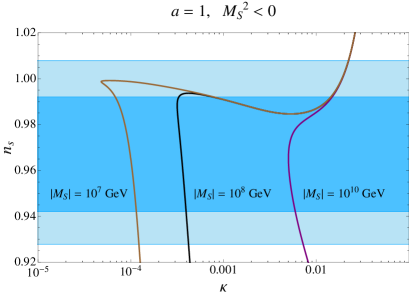
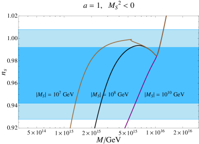
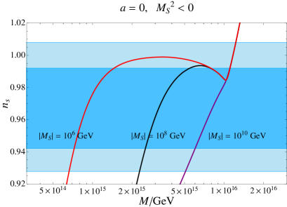
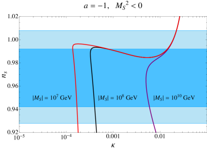
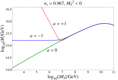
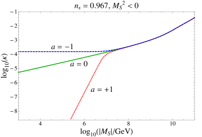
Using Eqs. (5)–(12), we have performed a series of numerical calculations to determine as a function of over a range of for the representative cases , and . Subsequently, we have calculated various other quantities (e.g. ) that depend on these parameters. The results of these calculations are presented in Figs. 1–3. We find that a red-tilted spectrum in good agreement with the WMAP5 central value, , is obtained for GeV in all cases of . For GeV, the coupling begins to take on large values (), supergravity corrections become increasingly important, and the spectral index approaches unity. The lowest value of leading to depends heavily upon .
The left (right) panels of Figs. 1, 2 and 3 show the behavior of with respect to () for , 0 and , respectively. In all of the cases depicted, a red tilted spectral index can be achieved, spanning the WMAP5 range for all values shown. As decreases, a clear trend toward smaller values of both and is exhibited. For the highest values of (say GeV), the -term is subdominant and all cases of are degenerate. This term begins to yield a sizable contribution around GeV and the predictions for begin to diverge, as seen in Fig. 4. In these panels, is held fixed at the central value 0.967 for ease in exploring an extended region of parameter space. For , we find that a red-tilted spectrum is possible for GeV. For , good agreement with WMAP5 can be obtained for values as low as the TeV scale. In the case of , the WMAP5 central value of can be obtained with arbitrarily small if we maintain that . As we have already mentioned, a suitably red-tilted spectrum can be obtained with even in the case of a slightly positive soft mass-squared term (i.e. TeV scale) [14], and so this result is expected. Indeed, for GeV, the -term begins to dominate over the mass-squared term, and no further significant change in behavior is exhibited. (This result was also seen in the full calculations where is free to vary.)
To understand the behavior exhibited in Fig. 4, it is useful to analytically examine some approximate formulae. For clarity, we will fix the spectral index at the central value for the purposes of this discussion. In the slow roll limit, the potential is dominated by the vacuum term, , and Eq. (11) becomes
| (16) |
For , the loop correction and soft mass-squared terms remain important for most values, until the SUGRA correction begins to dominate (around GeV) which drives the curve downward in Fig. 4(a). Taking the soft mass-squared term to be comparable to the loop correction term in and using the expression for in Eq. (13), we arrive at the following result
| (17) | |||||
| (18) |
where varies from 5 to 17 for – in order to obtain enough e-foldings.
As we have already noted, the curves corresponding to begin to diverge from the result at a scale around GeV, below which the linear soft SUSY-breaking term is important. The case is particularly interesting, as it generates values in a range which is important for proton decay considerations. In this case, the loop correction becomes supressed due to small values, as shown in Fig. 4(b); this greatly simplifies the analytical solution. Here we take the soft mass-squared term to be comparable to linear soft SUSY-breaking term in :
| (19) |
It turns out that the two soft terms cancel one another up to a few percent, and then their sum partially cancels with the SUGRA term to generate the measured curvature perturbation . We then obtain the following relations for in terms of and :
| (20) | |||||
| (21) |
For the case, the SUGRA and soft mass-squared terms become negligible below GeV, and the behavior of the curve decouples from . Taking the loop term to be comparable to the soft linear term, we obtain asymptotic and values given by
| (22) | |||||
| (23) |
where remains constant below GeV.
In addition to the spectral index , WMAP measures a variety of other quantities holding a great deal of information about the early universe. One such parameter, the tensor-to-scalar ratio , contains information about the amplitude of primordial gravitational waves, as well as the energy scale of inflation via . While current experimental bounds allow for a wide range of -values, this situation promises to improve in the near future with the recent launch of the Planck Surveyor. The SUSY hybrid models which we consider here predict exceedingly small values of ; in particular, the region corresponding to yields . This is a powerful statement in terms of upcoming precision measurements — if Planck measures a non-negligible value for , inflation models of this type will be convincingly ruled out.
It is interesting to note that the vacuum energy scale in these models takes on values that can be substantially smaller than the typical scale GeV. As a direct consequence, the -symmetry breaking scale turns out to be at most GeV for (i.e. for a U(1) model). In the flipped SU(5) model, however, can be significantly larger; as can be seen in Figs. 1(b), 2(b) and 3(b), this model leads to – GeV. This value acts as an upper bound for , and for GeV in the case. For , GeV, can be substantially larger than GeV (see Fig. 4(a)). However, this region of parameter space also corresponds to very low, possibly unnatural values of , as can be seen in Fig. 4(b).
It has recently been shown that similar scales, – GeV, are exhibited in the breaking of flipped SU(5) with threshold corrections taken into account [9]. In such models, a reduced proton lifetime of order yr is obtained in the channel , lying within the range to be probed by future planned experiments such as Hyper-K and DUSEL. According to Fig. 4(a), then, a SUSY hybrid model involving a negative soft mass-squared term of order – GeV appears to be in comfortable agreement with both WMAP and proton decay predictions. On the other hand, we find that – GeV for , with and . Choosing larger values in this case increases , yet this enhancement is not enough even for unnaturally large (e.g. GeV for ). Thus we see that is needed for consistency with proton decay considerations in a flipped SU(5) model.
Summary
In summary, we have explored the consequences of including the contribution of a sizable soft SUSY-breaking mass-squared term in the hybrid inflationary potential. As long as the physical inflaton mass is canonical, this soft term may be accompanied by a negative sign. If the magnitude of this soft mass is in an intermediate range, the WMAP5 central value of the spectral index (for ) may be obtained. The presence and sign of a soft linear term can also play a significant role; as this term becomes smaller and then negative, smaller values of lead to good agreement with the WMAP5 data. If these minimal models are embedded within a flipped SU(5) GUT, a symmetry breaking scale – GeV, which is consistent with a scalar spectral index –, leads to predictions of the proton lifetime of order – yrs. The model discussed here can be extended to other supersymmetric GUTs such as SU(5) and SO(10).
Acknowledgments
We thank Nefer Şenouz for valuable discussions. This work is supported in part by the DOE under grant No. DE-FG02-91ER40626, by the University of Delaware competitive fellowship (M.R.), and by NASA and the Delaware Space Grant Consortium under grant No. NNG05GO92H (J.W.).
 |
 |
| (a) | (b) |
 |
 |
| (a) | (b) |
 |
 |
| (a) | (b) |
 |
 |
| (a) | (b) |
References
- [1] G. R. Dvali, Q. Shafi, and R. K. Schaefer, Phys. Rev. Lett. 73, 1886 (1994), arXiv:hep-ph/9406319.
- [2] E. J. Copeland, A. R. Liddle, D. H. Lyth, E. D. Stewart, and D. Wands, Phys. Rev. D49, 6410 (1994), arXiv:astro-ph/9401011.
- [3] A. D. Linde, Phys. Rev. D49, 748 (1994), arXiv:astro-ph/9307002.
- [4] A. H. Chamseddine, R. L. Arnowitt, and P. Nath, Phys. Rev. Lett. 49, 970 (1982); R. Barbieri, S. Ferrara, and C. A. Savoy, Phys. Lett. B119, 343 (1982); L. J. Hall, J. D. Lykken, and S. Weinberg, Phys. Rev. D27, 2359 (1983); E. Cremmer, P. Fayet, and L. Girardello, Phys. Lett. B122, 41 (1983); N. Ohta, Prog. Theor. Phys. 70, 542 (1983).
- [5] V. N. Senoguz and Q. Shafi, Phys. Lett. B567, 79 (2003), arXiv:hep-ph/0305089.
- [6] R. Jeannerot, S. Khalil, G. Lazarides, and Q. Shafi, JHEP 10, 012 (2000), arXiv:hep-ph/0002151.
- [7] A. De Rujula, H. Georgi, and S. L. Glashow, Phys. Rev. Lett. 45, 413 (1980); H. Georgi, S. L. Glashow, and M. Machacek, Phys. Rev. D23, 783 (1981); S. M. Barr, Phys. Lett. B112, 219 (1982); J. P. Derendinger, J. E. Kim, and D. V. Nanopoulos, Phys. Lett. B139, 170 (1984); I. Antoniadis, J. R. Ellis, J. S. Hagelin, and D. V. Nanopoulos, Phys. Lett. B194, 231 (1987); Q. Shafi and Z. Tavartkiladze, Phys. Lett. B448, 46 (1999), arXiv:hep-ph/9811463; D. V. Nanopoulos (2002), arXiv:hep-ph/0211128.
- [8] B. Kyae and Q. Shafi, Phys. Lett. B635, 247 (2006), arXiv:hep-ph/0510105.
- [9] T. Li, D. V. Nanopoulos, and J. W. Walker (2009), arXiv:0910.0860.
- [10] J. Jiang, T. Li, D. V. Nanopoulos, and D. Xie (2008), arXiv:0811.2807; J. Jiang, T. Li, D. V. Nanopoulos, and D. Xie (2009), arXiv:0905.3394.
- [11] A. D. Linde and A. Riotto, Phys. Rev. D56, 1841 (1997), arXiv:hep-ph/9703209.
- [12] V. N. Senoguz and Q. Shafi, Phys. Rev. D71, 043514 (2005), arXiv:hep-ph/0412102; R. Jeannerot and M. Postma, JHEP 05, 071 (2005), arXiv:hep-ph/0503146.
- [13] G. R. Dvali, G. Lazarides, and Q. Shafi, Phys. Lett. B424, 259 (1998), arXiv:hep-ph/9710314.
- [14] M. U. Rehman, Q. Shafi, and J. R. Wickman, Phys. Lett. B [in press] (2009), arXiv:0908.3896.
- [15] WMAP, E. Komatsu et al., Astrophys. J. Suppl. 180, 330 (2009), arXiv:0803.0547.
- [16] M. Bastero-Gil, S. F. King, and Q. Shafi, Phys. Lett. B651, 345 (2007), arXiv:hep-ph/0604198; C. Pallis, JCAP 0904, 024 (2009), arXiv:0902.0334; B. Kyae (2009), arXiv:0910.4092.
- [17] M. ur Rehman, V. N. Senoguz, and Q. Shafi, Phys. Rev. D75, 043522 (2007), arXiv:hep-ph/0612023.
- [18] G. Lazarides and C. Pallis, Phys. Lett. B651, 216 (2007), arXiv:hep-ph/0702260.
- [19] M. U. Rehman, Q. Shafi, and J. R. Wickman, Phys. Rev. D79, 103503 (2009), arXiv:0901.4345.
- [20] H. P. Nilles, Phys. Rept. 110, 1 (1984).
- [21] J. L. Feng, A. Rajaraman, and B. T. Smith, Phys. Rev. D74, 015013 (2006), arXiv:hep-ph/0512172; R. Dermisek and H. D. Kim, Phys. Rev. Lett. 96, 211803 (2006), arXiv:hep-ph/0601036.
- [22] N. Arkani-Hamed and S. Dimopoulos, JHEP 06, 073 (2005), arXiv:hep-th/0405159; G. F. Giudice and A. Romanino, Nucl. Phys. B699, 65 (2004), arXiv:hep-ph/0406088; N. Arkani-Hamed, S. Dimopoulos, G. F. Giudice, and A. Romanino, Nucl. Phys. B709, 3 (2005), arXiv:hep-ph/0409232.
- [23] L. Boubekeur and D. H. Lyth, JCAP 0507, 010 (2005), arXiv:hep-ph/0502047; K. Kohri, C.-M. Lin, and D. H. Lyth, JCAP 0712, 004 (2007), arXiv:0707.3826.
- [24] B. Kyae and Q. Shafi, Phys. Lett. B597, 321 (2004), arXiv:hep-ph/0404168; B. Kyae and Q. Shafi, Phys. Rev. D72, 063515 (2005), arXiv:hep-ph/0504044.
- [25] G. F. Giudice and A. Masiero, Phys. Lett. B206, 480 (1988).
- [26] M. U. Rehman, Q. Shafi, and J. R. Wickman, Phys. Rev. D78, 123516 (2008), arXiv:0810.3625.
- [27] Q. Shafi and Z. Tavartkiladze (2006), arXiv:hep-ph/0606188.