Likelihood-free Bayesian inference for $\alpha$-stable models

Abstract

$\alpha$-stable distributions are utilised as models for heavy-tailed noise in many areas of statistics, finance and signal processing engineering. However, in general, neither univariate nor multivariate $\alpha$-stable models admit closed form densities which can be evaluated pointwise. This complicates the inferential procedure. As a result, $\alpha$-stable models are practically limited to the univariate setting under the Bayesian paradigm, and to bivariate models under the classical framework. In this article we develop a novel Bayesian approach to modelling univariate and multivariate $\alpha$-stable distributions based on recent advances in “likelihood-free” inference. We present an evaluation of the performance of this procedure in 1, 2 and 3 dimensions, and provide an analysis of real daily currency exchange rate data. The proposed approach provides a feasible inferential methodology at a moderate computational cost.

Keywords: $\alpha$-stable distributions; Approximate Bayesian computation; Likelihood-free inference; Sequential Monte Carlo samplers.

1 Introduction

Models constructed with $\alpha$-stable distributions possess several useful properties, including infinite variance, skewness and heavy tails ([Zolotarev 1986]; [Alder et al. 1998]; [Samorodnitsky and Taqqu 1994]; [Nolan 2007]). $\alpha$-stable distributions provide no general analytic expressions for the density, median, mode or entropy, but are uniquely specified by their characteristic function, which has several parameterizations. Considered as generalizations of the Gaussian distribution, they are defined as the class of location-scale distributions which are closed under convolutions. $\alpha$-stable distributions have found application in many areas of statistics, finance and signal processing engineering as models for impulsive, heavy tailed noise processes ([Mandelbrot 1960]; [Fama 1965]; [Fama and Roll 1968]; [Nikias and Shao 1995]; [Godsill 2000]; [Melchiori 2006]).

The univariate $\alpha$-stable distribution is typically specified by four parameters: $\alpha\in(0,2]$ determining the rate of tail decay; $\beta\in[-1,1]$ determining the degree and sign of asymmetry (skewness); $\gamma>0$ the scale (under some parameterizations); and $\delta\in\mathbb{R}$ the location [Levy 1924]. The parameter $\alpha$ is termed the characteristic exponent, with small and large $\alpha$ implying heavy and light tails respectively. Gaussian ($\alpha=2,\beta=0$) and Cauchy ($\alpha=1,\beta=0$) distributions provide the only analytically tractable sub-members of this family. In general, as $\alpha$-stable models admit no closed form expression for the density which can be evaluated pointwise (excepting Gaussian and Cauchy members), inference typically proceeds via the characteristic function.

This paper is concerned with constructing both univariate and multivariate Bayesian models in which the likelihood model is from the class of $\alpha$-stable distributions. This is known to be a difficult problem. Existing methods for Bayesian $\alpha$-stable models are limited to the univariate setting ([Buckle 1995]; [Godsill 1999]; [Godsill 2000]; [Lombardi 2007]; [Casarin 2004]; [Salas-Gonzalez et al. 2006]).

Inferential procedures for $\alpha$-stable models may be classified as auxiliary variable methods, inversion plus series expansion approaches and density estimation methods. The auxiliary variable Gibbs sampler [Buckle 1995] increases the dimension of the parameter space from $4$ ($\alpha,\beta,\gamma$ and $\delta$) to $n+4$, where $n$ is the number of observations. As strong correlations between parameters and large sample sizes are common in the $\alpha$-stable setting, this results in a slowly mixing Markov chain since Gibbs moves are limited to moving parallel to the axes (e.g. [Neal 2003]). Other Markov chain Monte Carlo (MCMC) samplers ([DuMouchel 1975, Lombardi 2007]) adopt inversion techniques for numerical integration of the characteristic function, employing inverse Fourier transforms combined with a series expansion [Bergstrom 1953] to accurately estimate distributional tails. This is performed at each iteration of the Markov chain to evaluate the likelihood, and is accordingly computationally intensive. In addition the quality of the resulting approximation is sensitive to the spacing of the fast Fourier transform grid and the point at which the series expansion begins ([Lombardi 2007]).

Univariate density estimation methods include integral representations [Zolotarev 1986], parametric mixtures ([Nolan 1997]; [McCulloch 1998]) and numerical estimation through splines and series expansions ([Nolan et al. 2001]; [Nolan 2008]). ?) approximates symmetric stable distributions using a mixture of Gaussian and Cauchy densities. ?) and ?) approximate the $\alpha$-stable density through spline polynomials, and ?) via a mixture of Gaussian distributions. Parameter estimation has been performed by an expectation-maximization (EM) algorithm [Lombardi and Godsill 2006] and by method of (partial) moments ([Press 1972, Weron 2006]). Implemented within an MCMC sampler, such density estimation methods would be highly computational.

None of the above methods easily generalize to the multivariate setting. It is currently only practical to numerically evaluate two dimensional $\alpha$-stable densities via inversion of the characteristic function. Here the required computation is a function of $\alpha$ and the number and spread of masses in the discrete spectral representation ([Nolan et al. 2001]; [Nolan 1997]). Beyond two dimensions this procedure becomes untenably slow with limited accuracy.

In this article we develop practical Bayesian inferential methods to fit univariate and multivariate $\alpha$-stable models. To the best of our knowledge, no practical Bayesian methods have been developed for the multivariate model as the required computational complexity increases dramatically with model dimension. The same is true of classical methods beyond two dimensions. Our approach is based on recent developments in “likelihood-free” inference, which permits approximate posterior simulation for Bayesian models without the need to explicitly evaluate the likelihood.

In Section 2 we briefly introduce likelihood-free inference and the sampling framework used in this article. Section 3 presents the Bayesian $\alpha$-stable model, with a particular focus on summary statistic specification, a critical component of likelihood-free inference. We provide an evaluation of the performance of the proposed methodology in Section 4, based on controlled simulation studies in 1, 2 and 3 dimensions. Finally, in Section 5 we demonstrate an analysis of real daily currency data under both univariate and multivariate settings, and provide comparisons with existing methods. We conclude with a discussion.

2 Likelihood-free models

Computational procedures to simulate from posterior distributions, $\pi(\theta|y)\propto\pi(y|\theta)\pi(\theta)$, of parameters $\theta\in\Theta$ given observed data $y\in\mathcal{X}$, are well established (e.g. [Brooks et al. 2010]). However when pointwise evaluation of the likelihood function $\pi(y|\theta)$ is computationally prohibitive or intractable, alternative procedures are required. Likelihood-free methods (also known as approximate Bayesian computation) permit simulation from an approximate posterior model while circumventing explicit evaluation of the likelihood function ([Tavaré et al. 1997]; [Beaumont et al. 2002]; [Marjoram et al. 2003]; [Sisson et al. 2007]; [Ratmann et al. 2009]).

Assuming data simulation $x\sim\pi(x|\theta)$ under the model given $\theta$ is easily obtainable, likelihood-free methods embed the posterior $\pi(y|\theta)$ within an augmented model

$$\pi_{LF}(\theta,x|y)\propto\pi_{\epsilon}(y|x,\theta)\pi(x|\theta)\pi(\theta),$$ (2.1)

where $x\sim\pi(x|\theta)$, $x\in{\mathcal{X}}$, is an auxiliary parameter on the same space as the observed data $y$. The function $\pi_{\epsilon}(y|x,\theta)$ is typically a standard smoothing kernel (e.g. [Blum 2009]) with scale parameter $\epsilon$, which weights the intractable posterior with high values in regions when the observed data $y$ and auxiliary data $x$ are similar. For example, uniform kernels are commonplace in likelihood-free models (e.g. [Marjoram et al. 2003, Sisson et al. 2007]), although alternatives such as Epanechnikov [Beaumont et al. 2002] and Gaussian kernels [Peters et al. 2008] provide improved efficiency. The resulting approximation to the true posterior target distribution

$$\pi_{LF}(\theta|y)\propto\int_{\mathcal{X}}\pi_{\epsilon}(y|x,\theta)\pi(x|\theta)\pi(\theta)dx=\pi(\theta)\mathbb{E}_{\pi(x|\theta)}[\pi_{\epsilon}(y|x,\theta)]$$ (2.2)

improves as $\epsilon$ decreases, and exactly recovers the target posterior as $\epsilon\rightarrow 0$, as then $\lim_{\epsilon\rightarrow 0}\pi_{\epsilon}(y|x,\theta)$ becomes a point mass at $y=x$ [Reeves and Pettitt 2005].

Posterior simulation from $\pi_{LF}(\theta|y)$ can then proceed via standard simulation algorithms, replacing pointwise evaluations of $\pi_{LF}(\theta|y)$ with Monte Carlo estimates through the expectation (2.2), based on draws $x^{1},\ldots,x^{P}\sim\pi(x|\theta)$ from the model (e.g. [Marjoram et al. 2003]). Alternatively, simulation from the joint posterior $\pi_{LF}(\theta,x|y)$ is available by contriving to cancel the intractable likelihoods $\pi(x|\theta)$ in sample weights or acceptance probabilities. For example, importance sampling from the prior predictive distribution $\pi(\theta,x)=\pi(x|\theta)\pi(\theta)$ results in an importance weight of $\pi_{LF}(\theta,x|y)/\pi(\theta,x)\propto\pi_{\epsilon}(y|x,\theta)$, which is free of likelihood terms. See ?) for a discussion of marginal and joint-space likelihood-free samplers.

In general, the distribution of $\pi(x|\theta)$ will be diffuse, unless $x$ is discrete and $\dim(x)$ is small. Hence, generating $x\sim\pi(\cdot|\theta)$ with $x\approx y$ is improbable for realistic datasets $y$, and as a result the degree of computation required for a good likelihood-free approximation $\pi_{LF}(\theta|y)\approx\pi(\theta|y)$ (i.e. with small $\epsilon$) will be prohibitive. In practice, the function $\pi_{\epsilon}(y|x,\theta)$ is expressed through low dimensional vectors of summary statistics, $S(\cdot)$, such that $\pi_{\epsilon}(y|x,\theta)$ weights the intractable posterior through (2.1) with high values in regions where $S(y)\approx S(x)$.

If $S(\cdot)$ is sufficient for $\theta$, then letting $\epsilon\rightarrow 0$ recovers $\pi_{LF}(\theta|y)=\pi(\theta|y)$ as before, but with more acceptable computational overheads, as $\dim(S(x))<<\dim(x)$. As sufficient summary statistics are generally unavailable, the use of non-sufficient statistics is commonplace. The effect of less efficient estimators of $\theta$ in (2.2) is a more diffuse approximation of $\pi(\theta|y)$. Hence the choice of summary statistics in any application is critical, with the ideal being low-dimensional, efficient and near-sufficient.

In this article, we implement the likelihood-free sequential Monte Carlo sampler of ?), detailed in Appendix A. As the class of particle-based algorithms is the most efficient currently available in likelihood-free computation (e.g. [McKinley et al. 2009]), and within this class, the sampler of ?) is the only one to allow non-uniform functions $\pi_{\epsilon}(y|x,\theta)$, this sampler provides the best combination of efficient simulation and flexible modelling.

3 Bayesian $\alpha$-stable models

We now develop univariate and multivariate Bayesian $\alpha$-stable models. Unlike existing methods, likelihood-free inference is independent of model parameterization.

3.1 Univariate $\alpha$-stable Models

Denote the characteristic function of $n$ i.i.d. univariate $\alpha$-stable distributed random variables $X_{1},\ldots,X_{n}$ by $\Phi_{X}(t).$ A popular and convenient parameterization is

$$\Phi_{X}\left(t\right)=\left\{\begin{array}[]{ll}\exp\left(i\delta t-\gamma^{\alpha}\left|t\right|^{\alpha}\left[1+i\beta\tan\frac{\pi\alpha}{2}\text{sgn}\left(t\right)\left(\left|\gamma t\right|^{1-\alpha}-1\right)\right]\right)&\text{ \ if }\alpha\neq 1\\ \exp\left(i\delta t-\gamma\left|t\right|\left[1+i\beta\frac{2}{\pi}\text{sgn}\left(t\right)\ln\left(\gamma\left|t\right|\right)\right]\right)&\text{ \ if }\alpha=1,\end{array}\right.$$ (3.1)

where $\text{sgn}\left(t\right)=\frac{t}{\left|t\right|}$ and $i^{2}=-1$ (e.g. [Samorodnitsky and Taqqu 1994]). Many alternative parameterizations are detailed in ?) and ?). Under (3.1), the intractable stable density function is continuous and unimodal, taking support on $\left(-\infty,0\right)$ if $\alpha<1,\beta=-1$; $\left(0,\infty\right)$ if $\alpha<1,\beta=1$ and $\left(-\infty,\infty\right)$ otherwise.

Efficient simulation of auxiliary data, $x\sim\pi(x|\theta)$, under the model is critical for the performance of likelihood-free methods (Section 2). Here, it is straightforward to generate $\alpha$-stable variates under the model defined by the characteristic function (3.1) (e.g. [Devroye 1986]; [Nolan 2007]). This approach is provided in Appendix B.

3.1.1 Summary statistics

A key component of likelihood-free inference is the availability of low-dimensional, efficient and near-sufficient summary statistics. Since $\alpha$-stable models can possess infinite variance ($\alpha>1$) and infinite mean ($\alpha<1$), this choice must be made with care. Here we present several candidate summary vectors, $S_{1}$–$S_{5}$, previously utilized for parameter estimation in the univariate $\alpha$-stable model. In Section 4 we evaluate the performance of these vectors, and provide informed recommendations for the choice of summary statistics under the likelihood-free framework.

$S_{1}$ McCulloch’s Quantiles
?) and ?) estimate model parameters based on sample quantiles, while correcting for estimator skewness due to the evaluation of $\widehat{q}_{p}(x)$, the $p^{th}$ quantile of $x$, with a finite sample. Here, the data $x_{(i)}$ are arranged in ascending order and matched with $\widehat{q}_{s(i)}(x)$, where $s\left(i\right)=\frac{2i-1}{2n}$. Linear interpolation to $p$ from the two adjacent $s(i)$ values then establishes $\widehat{q}_{p}(x)$ as a consistent estimator of the true quantiles. Inversion of the functions

$$\widehat{v}_{\alpha}=\frac{\widehat{q}_{0.95}(\cdot)-\widehat{q}_{0.05}(\cdot)}{\widehat{q}_{0.75}(\cdot)-\widehat{q}_{0.25}(\cdot)},\>\widehat{v}_{\beta}=\frac{\widehat{q}_{0.95}(\cdot)+\widehat{q}_{0.05}(\cdot)-2\widehat{q}_{0.5}(\cdot)}{\widehat{q}_{0.95}(\cdot)-\widehat{q}_{0.05}(\cdot)},\>\widehat{v}_{\gamma}=\frac{\widehat{q}_{0.75}(\cdot)-\widehat{q}_{0.25}(\cdot)}{\gamma}$$

then provides estimates of $\alpha,\beta$ and $\gamma$. Note that from a computational perspective, inversion of $v_{\alpha},v_{\beta}$ or $v_{\gamma}$ is not required under likelihood-free methods. Finally, we estimate $\delta$ by the sample mean $\bar{X}$ (when $\alpha>1$). Hence $S_{1}(x)=(\widehat{v}_{\alpha},\widehat{v}_{\beta},\widehat{v}_{\gamma},\bar{x}).$

$S_{2}$ Zolotarev’s Transformation
Based on a transformation of data from the $\alpha$-stable family $X\rightarrow Z$, ?) (p.16) provides an alternative parameterization of the $\alpha$-stable model $(\alpha,\beta,\gamma,\delta)\leftrightarrow(\nu,\eta,\tau)$ with a characteristic function of the form

$$\log\Phi_{Z}\left(t\right)=-\exp\left\{\nu^{-\frac{1}{2}}\left[\log\left|t\right|+\tau-i\frac{\pi}{2}\eta\,\text{sgn}\left(t\right)\right]+\mathbb{C}\left(\nu^{-\frac{1}{2}}-1\right)\right\},$$ (3.2)

where $\mathbb{C}$ is Euler’s constant, and where $\nu\geqslant\frac{1}{4}$, $\left|\eta\right|\leq\min\{1,2\sqrt{\nu}-1\}$ and $\left|\tau\right|<\infty.$ This parameterization has the advantage that logarithmic moments have simple expressions in terms of parameters to be estimated. For a fixed constant $0<\xi\leq\frac{1}{2}$ ([Zolotarev 1986] recommends $\xi=0.25$) and for integer $n/3$, the transformation is

$$Z_{j}=X_{3j-2}-\xi X_{3j-1}-(1-\xi)X_{3j},\qquad j=1,2,\ldots,n/3.$$

Defining $V_{j}=\log\left|Z_{j}\right|$ and $U_{j}=\text{sgn}(X_{j})$, estimates for $\nu,\eta$ and $\tau$ are then given by

$$\widehat{\nu}=\max\{\tilde{\nu},\left(1+\left|\widehat{\eta}\right|\right)^{2}/4\},\quad\widehat{\eta}=\mathbb{E}\left(U\right),\quad\widehat{\tau}=\mathbb{E}\left(V\right),$$

where $\tilde{\nu}=\frac{6}{\pi^{2}}S^{2}(V)-\frac{3}{2}S^{2}(U)+1$, using sample variances $S^{2}(V)$ and $S^{2}(U)$. As before, $\delta$ is estimated by $\bar{X}$ (for $\alpha>1$), and so $S_{2}(x)=(\widehat{\nu},\widehat{\eta},\widehat{\tau},\bar{x})$.

$S_{3}$ Press’s Method Of Moments
For $\alpha\neq 1$ and unique evaluation points $t_{1},t_{2},t_{3},t_{4}$, the method of moments equations obtained from $\log\Phi_{X}(t)$ can be solved to obtain ([Press 1972]; [Weron 2006])

$$\log(\widehat{\gamma}) = \frac{\log\left|t_{1}\right|\log(-\log\left|\Phi(t_{2})\right|)-\log\left|t_{2}\right|\log(-\log\left|\Phi(t_{1})\right|)}{\log\left|t_{1}/t_{2}\right|},\quad\widehat{\alpha}=\frac{\log\frac{\log\left|\Phi\left(t_{1}\right)\right|}{\log\left|\Phi\left(t_{2}\right)\right|}}{\log\left|t_{1}/t_{2}\right|}$$

$$\left.\widehat{\beta}\right|_{\widehat{\alpha},\widehat{\gamma}} = \frac{\widehat{u}\left(t_{4}\right)/t_{4}-\widehat{u}\left(t_{3}\right)/t_{3}}{(\left|t_{4}\right|^{\widehat{\alpha}-1}-\left|t_{3}\right|^{\widehat{\alpha}-1})\widehat{\gamma}^{\widehat{\alpha}}\tan\left(\frac{\widehat{\alpha}\pi}{2}\right)},\quad\left.\widehat{\delta}\right|_{\widehat{\alpha}}=\frac{\left|t_{4}\right|^{\widehat{\alpha}-1}\widehat{u}\left(t_{3}\right)/t_{3}-\left|t_{3}\right|^{\widehat{\alpha}-1}\widehat{u}\left(t_{4}\right)/t_{4}}{\left|t_{4}\right|^{\widehat{\alpha}-1}-\left|t_{3}\right|^{\widehat{\alpha}-1}}$$

where $\widehat{u}(t)=\tan^{-1}[\sum_{i=1}^{n}\cos(tx_{i})/\sum_{i=1}^{n}\sin(tx_{i})]$. We adopt the evaluation points $t_{1}=0.2,t_{2}=0.8,t_{3}=0.1$ and $t_{4}=0.4$ as recommended by ?), and accordingly obtain $S_{3}(x)=(\widehat{\alpha},\widehat{\beta},\widehat{\gamma},\widehat{\delta}).$

$S_{4}$ Empirical Characteristic Function
The empirical characteristic function, $\widehat{\Phi}_{X}(t)=\frac{1}{n}\sum_{j=1}^{n}e^{itX_{j}}$ for $t\in(-\infty,\infty)$, can be used as the basis for summary statistics when standard statistics are not available. E.g. this may occur through the non-existence of moment generating functions. Hence, we specify $S_{4}(x)=(\widehat{\Phi}_{X}(t_{1}),\ldots,\widehat{\Phi}_{X}(t_{20}))$ where $t_{i}\in\{\pm 0.5,\pm 1,\pm 1.5,\ldots,\pm 5\}$.

$S_{5}$ Mean, Quantiles and Kolmogorov-Smirnov Statistic
The Kolmogorov-Smirnov statistic is defined as $KS(X)=\sup_{z}|F^{X}_{n}(z)-F^{Y}_{n}(z)|$, the largest absolute deviation between the empirical cumulative distribution functions of auxiliary ($X$) and observed ($Y$) data, where $F^{X}_{n}(z)={1\over n}\sum_{i=1}^{n}I_{(X_{i}\leq z)}$ and $I_{(X_{i}\leq z)}=1$ if $X_{i}\leq z$ and 0 otherwise. We specify $S_{5}(x)=(\bar{x},\{\widehat{q}_{p}(x)\},KS(x))$, where the set of sample quantiles $\{\widehat{q}_{p}(x)\}$ is determined by $p\in\{0.01,0.05,0.1,0.15,\ldots,0.9,0.95,0.99\}$.

Likelihood-free inference may be implemented under any parameterization which permits data generation under the model, and for which the summary statistics are well defined. From the above $S_{1}$–$S_{5}$ are jointly well defined for $\alpha>1$. Hence, to complete the specification of the univariate $\alpha$-stable model we adopt the independent uniform priors $\alpha\sim\text{U}[1.1,2]$, $\beta\sim\text{U}[-1,1]$, $\gamma\sim\text{U}[0,300]$ and $\delta\sim\text{U}[-300,300]$ (e.g. [Buckle 1995]). Note that the prior for $\alpha$ has a restricted domain, reflecting the use of sample moments in $S_{1}$–$S_{3}$ and $S_{5}$. For $S_{4}$ we may adopt $\alpha\sim\text{U}(0,2]$.

3.2 Multivariate $\alpha$-stable Models

Bayesian model specification and simulation in the multivariate $\alpha$-stable setting is challenging ([Nolan et al. 2001]; [Nolan 2008]; [Samorodnitsky and Taqqu 1994]). Here we follow ?), who defines the multivariate model for the random vector $\bm{X}=(X_{1},\ldots,X_{d})\in\mathbb{R}^{d}$ through the functional equations

$$\sigma^{\alpha}\left(\mathbf{t}\right) = \int_{S_{d}}\left|\left\langle\mathbf{t},\mathbf{s}\right\rangle\right|^{\alpha}\Gamma\left(d\mathbf{s}\right);\quad\beta\left(\mathbf{t}\right)=\sigma^{-\alpha}\left(\mathbf{t}\right)\int_{S_{d}}\text{sgn}\left(\left\langle\mathbf{t},\mathbf{s}\right\rangle\right)\left|\left\langle\mathbf{t},\mathbf{s}\right\rangle\right|^{\alpha}\Gamma\left(d\mathbf{s}\right)$$

$$\mu\left(\mathbf{t}\right) = \left\{\begin{array}[]{ll}\left\langle\mathbf{t},\bm{\mu}^{0}\right\rangle&\text{ \ \ }\alpha\neq 1\\ \left\langle\mathbf{t},\bm{\mu}^{0}\right\rangle-\frac{2}{\pi}\int_{S_{d}}\left\langle\mathbf{t},\mathbf{s}\right\rangle\ln\left|\left\langle\mathbf{t},\mathbf{s}\right\rangle\right|\Gamma\left(d\mathbf{s}\right)&\text{ \ \ }\alpha=1\end{array}\right.$$

where $\bm{t}=(t_{1},\ldots,t_{d})$, $\bm{s}=(s_{1},\ldots,s_{d})$, $\left\langle\bm{t},\bm{s}\right\rangle=\sum_{i=1}^{d}t_{i}s_{i}$, $\mathbb{S}^{d}$ denotes the unit $d$-sphere, $\Gamma\left(d\mathbf{s}\right)$ denotes the unique spectral measure, and $\sigma^{\alpha}\left(\mathbf{t}\right)$ represents scale, $\beta\left(\mathbf{t}\right)$ skewness and $\mu\left(\mathbf{t}\right)$ location (through the vector $\bm{\mu}^{0}=(\mu_{1}^{0},\ldots,\mu_{d}^{0})$). Scaling properties of the functional equations, e.g. $\mu(r\mathbf{t})=r\mu(\mathbf{t})$, mean that it is sufficient to consider them on the unit sphere [Nolan 1997]. The corresponding characteristic function is

$$\Phi_{\mathbf{X}}\left(\mathbf{t}\right)=\mathbb{E}\exp\left(i\left\langle\mathbf{X},\mathbf{t}\right\rangle\right)=\exp\left(-I_{\mathbf{X}}\left(\mathbf{t}\right)+i\left\langle\bm{\mu}^{0},\mathbf{t}\right\rangle\right)$$

with $I_{\mathbf{X}}(\mathbf{t})={\textstyle\int_{\mathbb{S}^{d}}}\psi_{\alpha}\left(\left\langle\mathbf{t},\mathbf{s}\right\rangle\right)\Gamma(d\mathbf{s}),$ where the function $\psi_{\alpha}$ is given by

$$\psi_{\alpha}\left(u\right)=\left\{\begin{array}[]{ll}\left|u\right|^{\alpha}\left(1-i\text{sgn}\left(u\right)\tan\left(\frac{\pi\alpha}{2}\right)\right)&\text{ \ \ }\alpha\neq 1\\ \left|u\right|^{\alpha}\left(1-i\frac{2}{\pi}\text{sgn}\left(u\right)\ln\left|u\right|\right)&\text{ \ \ }\alpha=1.\end{array}\right.$$

The spectral measure $\Gamma(\cdot)$ and location vector $\bm{\mu}^{0}$ uniquely characterize the multivariate distribution ([Samorodnitsky and Taqqu 1994]) and carry essential information relating to the dependence between the elements of $\mathbf{X}$. The continuous spectral measure is typically well approximated by a discrete set of $k$ Dirac masses $\Gamma\left(\cdot\right)=\sum\limits_{j=1}^{k}w_{j}\delta_{\mathbf{s}_{j}}(\cdot)$ (e.g. [Byczkowski et al. 1993]) where $w_{j}$ and $\delta_{\mathbf{s}_{j}}(\cdot)$ respectively denote the weight and Dirac mass of the $j^{th}$ spectral mass at location $\mathbf{s}_{j}\in\mathbb{S}^{d}$. By simplifying the integral in $I_{\mathbf{X}}(\mathbf{t})$, computation with the characteristic function $\Phi_{\mathbf{X}}^{\ast}(\mathbf{t})=\exp\{-\sum_{j=1}^{k}w_{j}\psi_{\alpha}(\left\langle\mathbf{t},\mathbf{s}_{j}\right\rangle)\}$ becomes tractable and data generation from the distribution defined by $\Phi_{\mathbf{X}}^{\ast}(\bm{t})$ is efficient (Appendix B). As with the univariate case (3.1), standard parameterizations of $\Phi_{\mathbf{X}}^{\ast}\left(\mathbf{t}\right)$ will be discontinuous at $\alpha=1$, resulting in poor estimates of location and $\Gamma(\cdot)$. In the multivariate setting this is overcome by Zolotarev’s M-parameterization ([Nolan et al. 2001]; [Nolan 2008]). Although likelihood-free methods are parameterization independent, it is sensible to work with models with good likelihood properties.

In a Bayesian framework we parameterize the model via the spectral mass, which involves estimation of the weights $\bm{w}=(w_{1},\ldots,w_{k})$ and locations $\mathbf{s}_{1:k}\in\mathbb{S}^{d\times k}$ of $\Gamma(\cdot)$. For $k=2$ this corresponds to $\mathbf{s}_{i}=\left(\cos\phi_{i},\sin\phi_{i}\right)\in\mathbb{S}^{2}$. More generally, for $\mathbf{s}_{i}=\left(s_{i}^{1},\ldots,s_{i}^{d}\right)\in\mathbb{S}^{d}$, we use hyperspherical coordinates $\bm{\phi}_{i}=(\phi^{i}_{1},\ldots,\phi^{i}_{d-1})$, where

$$\phi_{d-1}^{i}=\tan^{-1}\left(\frac{s^{d}_{i}}{s^{d-1}_{i}}\right),\quad\ldots\quad,\quad\phi_{1}^{i}=\tan^{-1}\left(\frac{\sqrt{\left(s^{d}_{i}\right)^{2}+\left(s^{d-1}_{i}\right)^{2}+\ldots+\left(s^{2}_{i}\right)^{2}}}{s^{1}_{i}}\right).$$

We define priors for the parameters $\left(\bm{w},\bm{\phi}_{1:k},\bm{\mu}^{0},\alpha\right)$, with $\bm{\phi}_{1:k}=(\bm{\phi}_{1},\ldots,\bm{\phi}_{k})$, as $\bm{w}\sim\text{Dirichlet}(s,\ldots,s)$, $\phi_{j^{\prime}}^{i}\sim\text{U}(0,2\pi)$, $\mu_{j}^{0}\sim\text{N}(\xi,\kappa^{-1})$, $\alpha\sim\text{U}(0,2)$ for $i=1,\ldots,k$, $j=1,\dots,d$, $j^{\prime}=1,\ldots,d-1$ and impose the ordering constraint $s_{i-1}^{1}\leq s_{i}^{1}$ for all $i$ on the first element of each vector $\bm{s}_{i}$. Note that by treating the weights and locations of the spectral masses as unknown parameters, these may be identified with those regions of the spectral measure with significant posterior mass. This differs with the approach of ?) where the spectral mass is evaluated at a large number of deterministic grid locations. In estimating $\Gamma(\cdot)\mid\mathbf{X}$ a significant reduction in the number of required projection vectors is achieved (Sections 3.2.1 and 4.2). Further, the above prior specification does not penalize placement of spectral masses in close proximity. While this proved adequate for the presented analyses, alternative priors may usefully inhibit spectral masses at similar locations ([Pievatolo and Green 1998]).

3.2.1 Summary statistics

$S_{6}$ Nolan, Panorska & McCulloch Projection Method
For the $d$-variate $\alpha$-stable observations, $\mathbf{X}_{i},i=1,\ldots,n$, we take projections of $\mathbf{X}_{i}$ onto a unit hypersphere in the direction $\mathbf{t}\in\mathbb{S}^{d}$. This produces a set of $n$ univariate values, $\mathbf{X}^{\mathbf{t}}=(X^{\mathbf{t}}_{1},\ldots,X^{\mathbf{t}}_{n})$, where $X_{i}^{\mathbf{t}}=\left\langle\mathbf{X}_{i},\mathbf{t}\right\rangle$. The information in $\mathbf{X}^{\mathbf{t}}$ can then be summarized by any of the univariate summary statistics $S_{1}(\mathbf{X}^{\mathbf{t}}),\ldots,S_{5}(\mathbf{X}^{\mathbf{t}})$. This process is repeated for multiple projections over $\mathbf{t}_{1},\ldots,\mathbf{t}_{\tau}$. With the location parameter $\bm{\mu^{0}}$ estimated by $\bar{\mathbf{x}}$, for sufficient numbers of projection vectors, $\tau$, the summary statistics $S_{6}(\mathbf{X})=(\bar{\mathbf{x}},S_{s}(\mathbf{X}^{\mathbf{t}_{1}}),\ldots,S_{s}(\mathbf{X}^{\mathbf{t}_{\tau}}))$ for some $s\in\{1,2,3,4,5\}$, will capture much of the information contained in the multivariate data, if $S_{s}$ is itself informative. The best choice of univariate summary vector $S_{s}$ will be determined in Section 4.1. We adopt a randomized approach to the selection of the projection vectors $\mathbf{t}_{1},\ldots,\mathbf{t}_{\tau}$, avoiding curse of dimensionality issues as the dimension $d$ increases ([Nolan 2008]).

4 Evaluation of model and sampler performance

We now analyze the performance of the Bayesian $\alpha$-stable models and likelihood-free sampler in a sequence of simulation studies. For the univariate model, we evaluate the capability of the summary statistics $S_{1},\ldots,S_{5}$, and contrast the results with the samplers of ?) and ?). The performance of the multivariate model under the statistics $S_{6}$ is then considered for two and three dimensions.

In the following, we implement the likelihood-free sequential Monte Carlo algorithm of ?) (Appendix A) in order to simulate from the likelihood-free approximation to the true posterior $\pi_{LF}(\theta|y)\approx\pi(\theta|y)$ given by (2.2). This algorithm samples directly from $\pi_{LF}(\theta|y)$ using density estimates based on $P\geq 1$ Monte Carlo draws $x^{1},\ldots,x^{P}\sim\pi(x|\theta)$ from the model. We define $\pi_{\epsilon}(y|x,\theta)$ as a Gaussian kernel so that the summary statistics $S(y)\sim N(S(x),\epsilon^{2}\Sigma)$ for a suitably chosen $\Sigma$. All inferences are based on $N=1000$ particles drawn from $\pi_{LF}(\theta|y)$. Detail of algorithm implementation is removed to Appendix A for clarity of exposition.

4.1 Univariate summary statistics and samplers

We simulate $n=200$ observations, $y$, from a univariate $\alpha$-stable distribution with parameter values $\alpha=1.7$, $\beta=0.9$, $\gamma=10$ and $\delta=10$. We then implement the likelihood-free sampler targeting $\pi_{LF}(\theta|y)$ for each of the univariate summary statistics $S_{1}$-$S_{5}$ described in Section 3.1.1, with uniform priors for all parameters (Section 3.1). Alternative prior specifications were investigated ([Lombardi 2007]; [Nolan 1997]), with little impact on the results.

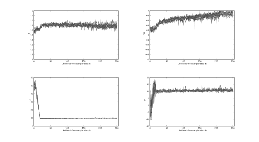
Figure 1: Traces of posterior MMSE estimates of $\alpha$, $\beta$, $\gamma$ and $\delta$ under the univariate $\alpha$-stable model and likelihood-free sampler (summary statistics $S_{1}$), based on 10 sampler replicates. Traces are shown as a function ($x$-axis) of sampler progression ($t$) and scale parameter reduction $\epsilon_{t}<\epsilon_{t-1}$. Parameter values used for data generation are $\alpha=1.7$, $\beta=0.9$, $\gamma=10$ and $\delta=10$.

Posterior minimum mean squared error (MMSE) estimates for each parameter, averaged over $10$ sampler replicates are detailed in Table 1. Monte Carlo standard errors are reported in parentheses. The results indicate that all summary vectors apart from $S_{5}$ estimate $\alpha$ and $\delta$ parameters well, and for $\gamma$, $S_{3}$ and $S_{4}$ perform poorly. Only $S_{1}$ gives reasonable results for $\beta$ and for all parameters jointly. Figure 1 illustrates a progression of the MMSE estimates of each parameter using $S_{1}$, from the likelihood-free SMC sampler output for each sampler replicate. As the sampler progresses, the scale parameter $\epsilon$ decreases, and the MMSE estimates identify the true parameter values as the likelihood-free posterior approximation improves.

The results in Table 1 are based on using $P=1$ Monte Carlo draws from the model to estimate $\pi_{LF}(\theta|y)$ (c.f. 2.2) within the likelihood-free sampler. Repeating the above study using $P\in\{5,10,20\}$ produced very similar results, and so we adopt $P=1$ for the sequel as the most computationally efficient choice.

For comparison, we also implement the auxiliary variable Gibbs sampler of ?) and the MCMC inversion and series expansion sampler of ?), based on chains of length 100,000 iterations (10,000 iterations burnin), and using their respective prior specifications. The Gibbs sampler performed poorly for most parameters. The MCMC method performed better, but has larger standard errors than the likelihood-free sampler using $S_{1}$.

The MCMC sampler [Lombardi 2007] performs likelihood evaluations via inverse Fast Fourier transform (FFT) with approximate tail evaluation using Bergstrom expansions. This approach is sensitive to $\alpha$, which determines the threshold between the FFT and the series expansion. Further, as the tail becomes fatter, a finer spacing of FFT abscissae is required to control the bias introduced outside of the Bergstrom series expansion, significantly increasing computation. Overall, this sampler worked reasonably for $\alpha$ close to 2, though with deteriorating performance as $\alpha$ decreased. The Gibbs sampler [Buckle 1995] performed extremely poorly for most settings and datasets, even when using their proposed change of variables transformations. As such, the results in Table 1 represent simulations under which both Gibbs and MCMC samplers performed credibly, thereby typifying their best case scenario performance.

4.2 Multivariate samplers

We consider varying numbers of discrete spectral masses, $k$, in the approximation to the spectral measure $\Gamma\left(\cdot\right)=\sum\limits_{j=1}^{k}w_{j}\delta_{\mathbf{s}_{j}}(\cdot).$ We assume that the number of spectral masses is known a priori, and denote the $d$-variate $\alpha$-stable distribution by $\bm{S}_{\alpha}\left(d,k,\bm{w},\bm{\phi}_{1:k},\bm{\mu}^{0}\right)$. Priors are specified in Section 3.2. Following the analysis of Section 4.1, we incorporate $S_{1}$ within the summary vector $S_{6}$.

For datasets of size $n=200$, we initially consider the performance of the bivariate $\alpha$-stable model, $\bm{S}_{\alpha}\left(2,k,\bm{w},\bm{\phi}_{1:k},\bm{0}\right)$, for $k=2$ and $3$ spectral masses, with respect to parameter estimation and the impact of the number of projection vectors $\mathbf{t}_{1},\ldots,\mathbf{t}_{\tau}$.

The true and mean MMSE estimates of each parameter, placing projection vectors at the true locations of the spectral masses, are presented in Table 2. In addition, results are detailed using $\tau=2,5,10$ and $20$ randomly (uniformly) placed projection vectors, in order to evaluate the impact of spectral mass location uncertainty. The likelihood-free sampler output results in good MMSE parameter estimates, even for 2 randomly placed projection vectors. The parameter least accurately estimated is the location vector, $\bm{\mu}^{0}$. Directly summarized by a sample mean in $S_{6}(\cdot)$, estimation of location requires a large number of observations when the data have heavy tails.

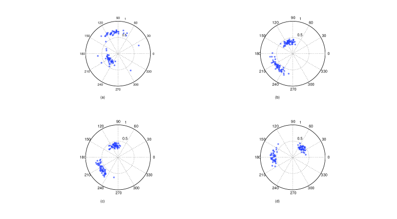
Figure 2: Circular scatter plot of MMSE estimates for $k=2$ spectral mass angles (angle) and weights (radius) for bivariate $\alpha$-stable $\bm{S}_{\alpha}\left(2,2,\bm{w},\bm{\phi}_{1:2},\bm{0}\right)$ model, with $\alpha=1.7$, $\bm{w}=(0.4,0.6)$ and $\bm{\phi}_{1:2}=(\pi/4,\pi)$. Plots (a)–(d) demonstrate evolution of the estimates for decreasing scale parameter values $\epsilon$, based on 10 sampler replicates.

Figure 2 illustrates progressive sampler performance for the $\bm{S}_{\alpha}\left(2,2,\bm{w},\bm{\phi}_{1:2},\bm{0}\right)$ model, with $\alpha=1.7$, $\bm{w}=(\pi/4,\pi)$ and $\bm{\phi}_{1:2}=(\pi/4,\pi)$. Each circular scatter plot presents MMSE estimates of weight (radius) and angles (angle) of the two spectral masses, based on 10 sampler replicates. The sequence of plots (a)–(d) illustrates the progression of the parameter estimates as the scale parameter $\epsilon$ (of $\pi_{\epsilon}(y|x,\theta)$) decreases (and hence the accuracy of the likelihood-free approximation $\pi_{LF}(\theta|y)\approx\pi(\theta|y)$ improves). As $\epsilon$ decreases, there is a clear movement of the MMSE estimates towards the true angles and weights, indicating appropriate sampler performance.

With simulated datasets of size $n=400$, we extend the previous bivariate study to 3 dimensions, with $k=2$ discrete spectral masses. The true parameter values, and posterior mean MMSE estimates and associated standard errors, based on 10 sampler replicates, are presented in Table 3. Again, reasonable parameter estimates are obtained (given finite data), with location ($\bm{\mu}^{0}$) again the most difficult to estimate.

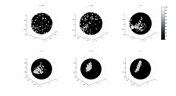
Figure 3: Spherical heat map of MMSE estimates for the first of $k=2$ discrete spectral masses, $\bm{\phi}_{1}$, for the trivariate $\alpha$-stable $\bm{S}_{\alpha}\left(3,2,\bm{w},\bm{\phi}_{1:2},\bm{0}\right)$ model. True values of the first spectral mass are $w_{1}=0.7$ (70%) and $\bm{\phi}_{1}=(\pi/4,\pi)$. Point shading indicates MMSE value of $w_{1}$ as a percentage. The plots demonstrate the evolution of the estimates for decreasing scale parameter values $\epsilon$, based on 200 sampler replicates.

In analogy with Figure 2, progressive sample performance for the first spectral mass (with $w_{1}=0.7$ and $\bm{\phi}_{1}=(\pi/4,\pi))$ for decreasing scale parameter $\epsilon$ is shown in Figure 3. Based on 200 replicate MMSE estimates (for visualization purposes), the shading of each point indicates the value of $w_{1}$ as a percentage (black=0%, white=100%), and the location on the sphere represents the angles $\bm{\phi}_{1}$. For large $\epsilon$, the MMSE estimates for location are uniformly distributed over the sphere, and the associated weight takes the full range of possible values, $0-100$%. As $\epsilon$ decreases, the estimates of spectral mass location and weight become strongly localized and centered on the true parameter values, again indicating appropriate sampler performance. Similar images are produced for the second discrete spectral mass.

5 Analysis of exchange rate daily returns

Our data consist of daily exchange rates for 5 different currencies recorded in GBP between 1 January 2005 and 1 December 2007. The data involve 1065 daily-averaged LIBOR (London interbank offered rate) observations $y^{\prime}_{1},\ldots,y^{\prime}_{1065}$. The standard log-transform generates a log returns series $y_{t}=\ln\left(y^{\prime}_{t+1}/y^{\prime}_{t}\right)$. Cursory examination of each returns series reveals clear non-Gaussian tails and/or skewness (Table 4, bottom).

We initially model each currency series as independent draws from a univariate $\alpha$-stable distribution. Posterior MMSE parameter estimates for each currency are given in Table 4, based on 10 replicate likelihood-free samplers using the $S_{1}$ summary vector. For comparison, we also compute McCulloch’s sample quantile based estimates (derived from $S_{1}$, c.f. Section 3.1.1), and maximum likelihood estimates using J. P. Nolan’s STABLE program (available online), using the direct search SPDF option with search domains given by $\alpha\in(0.4,2]$, $\beta\in[-1,1]$, $\gamma\in[0.00001,1]$ and $\delta\in[-1,1]$. Overall, there is good agreement between Bayesian, likelihood- and sample-based estimators. All currency returns distributions are significantly different from Gaussian ($\alpha=2,\beta=0$), and exhibit similar family parameter $(\alpha)$ estimates over this time period. However, the GBP to YEN conversion demonstrates a significantly asymmetry ($\beta$) compared to the other currencies.

An interesting difference between the methods of estimation, is that McCulloch’s estimates of $\alpha$ differ considerably from the posterior MMSE estimates, even though the latter are constructed using McCulloch’s estimates directly as summary statistics, $S_{1}$. One reason that the Bayesian estimates are more in line with the MLE’s, is that likelihood-free methods largely ignore bias in estimators used as summary statistics (comparing the closeness between biased or unbiased estimators will produce similar results – consider comparing sample and maximum likelihood estimators of variance).

The multivariate $\alpha$-stable distribution assumes that its marginal distributions, which are also $\alpha$-stable, possess identical shape parameters. This property implies important practical limitations, one of which is that it is only sensible to jointly model data with similar marginal shape parameters. Accordingly, based on Table 4, we now consider a bivariate analysis of AUD and EURO currencies. Restricting the analysis to the bivariate setting also permits comparison with the bivariate frequentist approach described in ?) using the MVSTABLE software (available online).

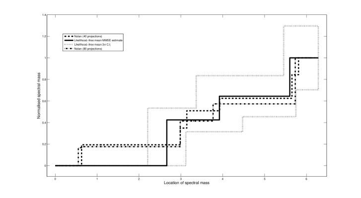
Figure 4: Estimates of spectral mass location (x-axis) and cumulative weight (y-axis) for AUD and EURO currencies data. Solid line denotes mean posterior MMSE estimates of likelihood-free SMC sampler output, and dotted line illustrates mean $3\sigma$ posterior credibility intervals, based on $k=3$ discrete spectral masses, 20 randomly placed projection vectors and 10 replicate samplers. Broken lines denote estimate of spectral mass using J. P. Nolan’s MVSTABLE software, available at academic2.american.edu/$\sim$jpnolan, with (dashed line) 40 deterministic projection locations and (dash-dot line) 80 projection locations.

A summary illustration of the discrete approximations to the underlying continuous spectral mass is shown in Figure 4. Assuming $k=3$ discrete spectral masses and based on 10 likelihood-free sampler replicates, the mean MMSE posterior estimates (solid black line) with mean $3\sigma$ posterior credibility intervals (dotted line), identify regions of high spectral mass located at 2.7, 3.9 and 5.6, with respective weights 0.45, 0.2 and 0.35. Broken lines in Figure 4 denote the frequentist estimates of ?), based on the identification of mass over an exhaustive mesh grid using 40 (dashed line) and 80 (dash-dot line) prespecified grid locations (projections).

Overall, both approaches produce comparable summary estimates of the spectral mass approximation, although the likelihood-free models generate full posterior distributions, compared to Nolan’s frequentist estimates. The assumption of $k=3$ discrete spectral masses provides a parsimonious representation of the actual spectral mass. For example, the spectral mass located at 2.7 accounts for the first two/three masses based on Nolan’s estimates (80/40 projections). While the frequentist approach is computationally restricted to bivariate inference, the likelihood-free approach may naturally be applied in much higher dimensions.

6 Discussion

Statistical inference for $\alpha$-stable models is challenging due to the computational intractability of the density function. In practice this limits the range of models fitted, to univariate and bivariate cases. By adopting likelihood-free Bayesian methods we are able to circumvent this difficulty, and provide approximate, but credible posterior inference in the general multivariate case, at a moderate computational cost. Critical to this approach is the availability of informative summary statistics for the parameters. We have shown that multivariate projections of data onto the unit hypersphere, in combination with sample quantile estimators, are adequate for this task.

Overall, our approach has a number of advantages over existing methods. There is far greater sampler consistency than alternative samplers, such as the auxiliary Gibbs or MCMC inversion plus series expansion samplers ([Buckle 1995]; [Lombardi 2007]). It is largely independent of the complexities of the various parameterizations of the $\alpha$-stable characteristic function. The likelihood-free approach is conceptually straightforward, and scales simply and is easily implemented in higher dimensions (at a higher computational cost). Lastly, by permitting a full Bayesian multivariate analysis, the component locations and weights of a discrete approximation to the underlying continuous spectral density are allowed to identify those regions with highest posterior density in a parsimonious manner. This is a considerable advantage over highly computational frequentist approaches, which require explicit calculation of the spectral mass over a deterministic and exhaustive grid (e.g. [Nolan 1997]).

Each analysis in this article used many millions of data-generations from the model. While computation for likelihood-free methods increases with model dimension and desired accuracy of the model approximation (through $\epsilon$), much of this can be offset through parallelization of the likelihood-free sampler [Peters et al. 2008].

Finally, while we have largely focused on fitting $\alpha$-stable models in the likelihood-free framework, extensions to model selection through Bayes factors or model averaging are immediate. One obvious candidate in this setting is the unknown number of discrete spectral masses, $k$, in the approximation to the continuous spectral density.

Acknowledgments

YF and SAS are supported by the Australian Research Council Discovery Project scheme (DP0877432 & DP1092805). GWP is supported by an APA scholarship and by the School of Mathematics and Statistics, UNSW and CSIRO CMIS. We thank M. Lombardi for generously providing the use of his code [Lombardi 2007], and M. Briers, S. Godsill, Xiaolin Lou, P. Shevchenko and R. Wolpert, for thoughtful discussions.

Appendix A

SMC sampler PRC-ABC algorithm [Peters et al. 2008]  

Initialization:

Set $t=1$ and specify tolerance schedule $\epsilon_{1},\ldots,\epsilon_{T}$.
For $i=1,\ldots,N$, sample $\theta^{(i)}_{1}\sim\pi(\theta)$, and set weights $W_{1}(\theta^{(i)}_{1})=\pi_{LF,1}(\theta_{1}^{(i)}|y)/\pi(\theta^{(i)}_{1})$.

Resample:

Resample $N$ particles with respect to $W_{t}(\theta_{t}^{(i)})$ and set $W_{t}(\theta_{t}^{(i)})=\frac{1}{N},\\ i=1,\ldots,N$.

Mutation and correction:

Set $t=t+1$ and $i=1$:
(a) Sample $\theta_{t}^{(i)}\sim M_{t}(\theta_{t})$ and set weight for $\theta_{t}^{(i)}$ to     $W_{t}(\theta_{t}^{(i)})=\pi_{LF,t}(\theta_{t}^{(i)}|y)/M_{t}(\theta_{t}^{(i)})$. (b) With probability $1-p^{(i)}=1-\min\{1,W_{t}(\theta_{t}^{(i)})/c_{t}\}$, reject $\theta_{t}^{(i)}$ and go to (a). (c) Otherwise, accept $\theta_{t}^{(i)}$ and set $W_{t}(\theta_{t}^{(i)})=W_{t}(\theta_{t}^{(i)})/p^{(i)}$. (d) Increment $i=i+1$. If $i\leq N$, go to (a). (e) If $t<T$ then go to Resample.

 

This algorithm samples $N$ weighted particles from a sequence of distributions $\pi_{LF,t}(\theta|y)$ given by (2.2), where $t$ indexes a sequence of scale parameters $\epsilon_{1}\geq\ldots\geq\epsilon_{T}$. The final particles $\{(W_{T}(\theta^{(i)}_{T}),\theta_{T}^{(i)}):i=1,\ldots,N\}$, form a weighted sample from the target $\pi_{LF,T}(\theta|y)$ (e.g. [Peters et al. 2008]). The densities $\pi_{LF,t}(\theta|y)$ are estimated through the Monte Carlo estimate of the expectation (2.2) based on $P$ draws $x^{1},\ldots,x^{P}\sim\pi(x|\theta)$.

For the simulations presented we implement the following specifications: for univariate $\alpha$-stable models $\theta=(\alpha,\beta,\gamma,\delta)$ and for multivariate models $\theta=(\bm{w},\bm{\phi}_{1:k},\bm{\mu}^{0},\alpha)$; we use $N=1000$ particles, initialized with samples from the prior; the function $\pi_{\epsilon}(y|x,\theta)$ is defined by $S(y)\sim N(S(x),\epsilon^{2}\hat{\Sigma})$ where $\hat{\Sigma}$ is an estimate of $\mbox{Cov}(S(x)|\hat{\theta})$ based on 1000 draws $x^{1},\ldots,x^{1000}\sim\pi(x|\hat{\theta})$ given an approximate maximum likelihood estimate $\hat{\theta}$ of $\theta$ [Jiang and Turnbull 2004]; the mutation kernel $M_{t}(\theta_{t})=\sum_{i=1}^{N}W^{(i)}_{t-1}(\theta^{(i)}_{t-1})\phi(\theta_{t};\,\theta^{(i)}_{t-1},\Lambda)$ is a density estimate of the previous particle population $\{(W_{t-1}(\theta^{(i)}_{t-1}),\theta_{t-1}^{(i)}):i=1,\ldots,N\}$, with a Gaussian kernel density $\phi$ with covariance $\Lambda$; for univariate $\alpha$-stable models $\Lambda=\mbox{diag}(0.25,0.25,1,1)$, and for multivariate models $\Lambda=\mbox{diag}(1,\ldots,1,0.25)$ (with Dirichlet proposals and kernel density substituted for $\bm{w}$); the sampler particle rejection threshold is adaptively determined as the $90^{th}$ quantile of the weights $c_{t}=\widehat{q}_{0.9}(\{W^{(i)}_{t}(\theta_{t}^{(i)})\}),$ where $\{W^{(i)}_{t}(\theta_{t}^{(i)})\}$ are the $N$ particle weights prior to particle rejection (steps (b) and (c)) at each sampler stage $t$ (see [Peters et al. 2008]).

For each analysis we implement 10 independent samplers (in order to monitor algorithm performance and Monte Carlo variability), each with the deterministic scale parameter sequence: $\epsilon_{t}\in\{1000,900,\ldots,200,100,99,\ldots,11,10,9.5,9,\ldots,5.5,5,4.95,$ $\ldots,3.05,3,2.99,2.98,\ldots,0.01,0\}$. However, we adaptively terminate all samplers at the largest $\epsilon$ value such that the effective sample size (estimated by $[\sum_{i=1}^{N}[W^{(i)}_{t}(\theta_{t}^{(i)})]^{2}]^{-1}$) consistently drops below $0.2N$ over all replicate sampler implementations.

Appendix B: Data generation

Simulation of univariate $\alpha$-stable data ([DuMouchel 1975], [Chambers et al. 1976])

1. Sample $W\sim\mbox{Exp}(1)$ to obtain $w$

2. Sample $U\sim\mbox{Uniform}[-\pi/2,\pi/2]$ to obtain $u$

3. Apply transformation to obtain sample $\overline{y}$

   $$\overline{y}=\left\{\begin{array}[c]{cll}&S_{\alpha,\beta}\frac{\sin\alpha\left(u+B_{\alpha,\beta}\right)}{(\cos u)^{\alpha/2}}\left[\frac{\cos\left(u-\alpha\left(u+B_{\alpha,\beta}\right)\right)}{w}\right]^{\frac{1-\alpha}{\alpha}}&\text{ \ \ if }\alpha\neq 1\\ &\frac{2}{\pi}\left[\left(\frac{\pi}{2}+\beta u\right)\tan u-\beta\ln\frac{\frac{\pi}{2}w_{i}\cos u}{\frac{\pi}{2}+\beta u}\right]&\text{ \ \ if }\alpha=1\end{array}\right.$$

   with $S_{\alpha,\beta}=\left(1+\beta^{2}\tan^{2}\left(\frac{\pi\alpha}{2}\right)\right)^{-1/2\alpha}$ and $B_{\alpha,\beta}=\frac{1}{\alpha}\arctan\left(\beta\tan\left(\frac{\pi\alpha}{2}\right)\right).$ In this case $\overline{y}$ will have distribution defined by $\Phi_{X}\left(t\right)$ with parameters $\left(\alpha,\beta,1,0\right)$.

4. Apply transformation to obtain sample $y=\gamma\overline{y}+\delta$ with parameters $\left(\alpha,\beta,\gamma,\delta\right)$.

Simulation of $d$-dimensional, multivariate $\alpha$-stable data ([Nolan 2007])

1. Generate $Z_{1},...,Z_{k}$ i.i.d. random variables from the univariate $\alpha$-stable distribution with parameters $(\alpha,\beta,\gamma,\delta)=(\alpha,1,1,0)$.

2. Apply the transformation

   $$Y\mathbf{=}\left\{\begin{array}[]{ll}\sum\limits_{j=1}^{k}w_{j}^{1/\alpha}Z_{j}\mathbf{s}_{j}+\bm{\mu}^{0}\text{ \ \ }&\alpha\neq 1\\ \sum\limits_{j=1}^{k}w_{j}\left(Z_{j}+\frac{2}{\pi}\ln\left(w_{j}\right)\right)\mathbf{s}_{j}+\bm{\mu}^{0}\text{ \ \ }&\alpha=1\end{array}\right.$$

with $\bm{s}_{1},\ldots,\bm{s}_{k},\bm{\mu}^{0}\in\mathbb{S}^{d}$. Note that while the complexity for generating realizations from a multivariate $\alpha$-stable distribution is linear in the number of point masses ($k$) in the spectral representation per realization, this method is strictly only exact for discrete spectral measures.

	Buckle	Lombardi	$S_{1}$	$S_{2}$	$S_{3}$	$S_{4}$	$S_{5}$
$\alpha$ (1.7)	1.77 (0.18)	1.62 (0.10)	1.69 (0.06)	1.65 (0.07)	1.70 (0.06)	1.71 (0.04)	1.56 (0.05)
$\beta$ (0.9)	0.54 (0.21)	0.86 (0.18)	0.86 (0.10)	0.65 (0.13)	0.31 (0.09)	0.38 (0.12)	0.49 (0.11)
$\gamma$ (10.0)	18.17 (6.19)	9.59 (2.16)	9.79 (0.21)	10.44(0.56)	38.89 (6.34)	39.12 (5.92)	9.34 (0.14)
$\delta$ (10.0)	12.30 (4.12)	9.70 (2.19)	10.64 (0.83)	9.31 (0.86)	10.25 (0.98)	10.83 (1.34)	11.18 (1.05)

Table 1: Means and standard errors (in parentheses) of posterior MMSE estimates of $\alpha$, $\beta$, $\gamma$ and $\delta$ under the univariate $\alpha$-stable model, based on 10 sampler replicates. Parameter values used for data simulation are given in the left column. Comparisons are between the auxiliary variable Gibbs sampler method of Buckle (1995), the inversion MCMC method of Lombardi (2007), and the likelihood-free method, using summary statistics $S_{1}$–$S_{5}$.

	$\alpha$	$\mu_{1}^{0}$	$\phi^{1}$	$\phi^{2}$	$\phi^{3}$	$w_{1}$	$w_{2}$	$w_{3}$
True: $k=2$	1.7	0	$\frac{\pi}{4}$	$\pi$	–	0.6	0.4	–
True: $k=3$	1.7	0	$\frac{\pi}{4}$	$\pi$	$\frac{3\pi}{2}$	0.3	0.25	0.45
$k$	$\widehat{\alpha}$	$\widehat{\mu_{1}^{0}}$	$\widehat{\phi^{1}}$	$\widehat{\phi^{2}}$	$\widehat{\phi^{3}}$	$\widehat{w_{1}}$	$\widehat{w_{2}}$	$\widehat{w_{3}}$
Projection vectors at locations of true spectral masses.
2	1.66 (0.04)	0.16 (0.19)	0.81 (0.65)	3.19 (0.46)	–	0.55 (0.06)	0.45 (0.05)	–
3	1.79 (0.02)	0.36 (0.18)	0.84 (0.27)	3.18 (0.29)	4.91 (0.24)	0.35 (0.05)	0.25 (0.04)	0.40 (0.05)
2 projection vectors
2	1.67 (0.06)	-0.13 (0.16)	0.73 (0.55)	3.58 (0.57)	–	0.58 (0.09)	0.42 (0.10)	–
3	1.76 (0.05)	-0.16 (0.26)	0.91 (0.66)	3.65 (0.62)	4.85 (0.55)	0.36 (0.10)	0.24 (0.09)	0.40 (0.08)
5 projection vectors
2	1.71 (0.05)	0.08 (0.14)	0.71 (0.60)	3.80 (0.67)	–	0.60 (0.07)	0.40 (0.09)	–
3	1.75 (0.04)	0.29 (0.17)	0.86 (0.62)	3.68 (0.52)	4.82 (0.41)	0.35 (0.09)	0.20 (0.07)	0.42 (0.09)
10 projection vectors
2	1.72 (0.02)	0.21 (0.21)	0.75 (0.32)	3.31 (0.32)	–	0.59 (0.05)	0.41 (0.07)	–
3	1.73 (0.03)	0.25 (0.16)	0.76 (0.44)	3.31 (0.48)	4.78 (0.19)	0.34 (0.07)	0.24 (0.04)	0.42 (0.05)
20 projection vectors
2	1.71 (0.03)	-0.14 (0.14)	0.76 (0.36)	3.21 (0.23)	–	0.63 (0.03)	0.37 (0.03)	–
3	1.72 (0.02)	0.18 (0.23)	0.77 (0.32)	3.25 (0.31)	4.75 (0.15)	0.34 (0.04)	0.23 (0.03)	0.43 (0.03)

Table 2: Mean MMSE parameter estimates (and standard errors) for the bivariate $\alpha$-stable $\bm{S}_{\alpha}\left(2,k,\bm{w},\bm{\phi}_{1:k},\bm{\mu}^{0}\right)$ model, for $k=2,3$ discrete spectral masses, calculated over $10$ replicate samplers. Projections vectors are placed at the true, and 2, 5, 10 and 20 randomly selected spectral mass locations. The true value of $\bm{\mu}^{0}$ is the origin.

	$\alpha$	$\mu_{1}^{0}$	$\phi_{1}^{1}$	$\phi_{2}^{1}$	$\phi_{1}^{2}$	$\phi^{2}_{2}$	$w_{1}$	$w_{2}$
True: $k=2$	1.7	0	$\frac{\pi}{4}$	$\pi$	$\frac{\pi}{2}$	$\frac{3\pi}{2}$	0.3	0.7
$k$	$\widehat{\alpha}$	$\widehat{\mu_{1}^{0}}$	$\widehat{\phi_{1}^{1}}$	$\widehat{\phi_{2}^{1}}$	$\widehat{\phi_{1}^{2}}$	$\widehat{\phi_{2}^{2}}$	$\widehat{w_{1}}$	$\widehat{w_{2}}$
20 projection vectors
2	1.71 (0.02)	0.53 (0.89)	1.12 (0.34)	3.81 (0.45)	1.84 (0.54)	4.24 (0.69)	0.28 (0.06)	0.72 (0.05)

Table 3: Mean MMSE parameter estimates (and standard errors) for the trivariate $\alpha$-stable $\bm{S}_{\alpha}\left(3,2,\bm{w},\bm{\phi}_{1:2},\bm{\mu}^{0}\right)$ model, with $k=2$ discrete spectral masses, calculated over $10$ replicate samplers. The true value of $\bm{\mu}^{0}$ is the origin.

		Currency Exchange from GBP to
		AUD	CNY	EURO	YEN	USD
	$\widehat{\alpha}$	1.56 (0.03)	1.57 (0.02)	1.62 (0.04)	1.51 (0.04)	1.53 (0.02)
Likelihood	$\widehat{\beta}$	0.06 (0.03)	0.01 (0.009)	-0.007 (0.08)	-0.26 (0.09)	-0.04 (0.03)
free	$\widehat{\gamma}$	0.004 (4e-4)	0.003 (2e-4)	0.004 (1e-4)	0.003 (1e-4)	0.004 (3e-4)
	$\widehat{\delta}$	0.02 (0.01)	0.001 (0.0006)	-0.03 (0.09)	-0.06 (0.08)	-0.02 (0.07)
	$\widehat{\alpha}$	1.61 (0.05)	1.50 (0.05)	1.65 (0.05)	1.66 (0.04)	1.57 (0.05)
MLE	$\widehat{\beta}$	0.08 (0.11)	-0.01 (0.10)	-0.10 (0.12)	-0.46 (0.11)	-0.01 (0.11)
	$\widehat{\gamma}$	0.002 (7e-5)	0.002 (6e-5)	0.001 (4e-5)	0.002 (4e-5)	0.002 (1e-4)
	$\widehat{\delta}$	-2e-4 (1e-4)	-2e-5 (1e-4)	8e-5 (7e-5)	6e-4 (1e-4)	5e-5 (9e-5)
McCulloch’s	$\widehat{\alpha}$	1.39	1.38	1.47	1.38	1.39
quantile	$\widehat{\beta}$	0.08	-0.003	-0.04	-0.18	0.001
estimates	$\widehat{\gamma}$	0.002	0.002	0.001	0.002	0.002
	$\widehat{\delta}$	-4e-5	1e-6	1e-5	2e-4	5e-7
Kurtosis		8.39	9.11	15.60	6.29	4.98
Skewness		0.69	-0.42	-0.03	-0.79	0.11
Std. dev.		0.004	0.004	0.003	0.004	0.003
Mean		-4e-5	-4e-5	-9e-6	1e-4	7e-5

Table 4: Posterior MMSE estimates (Monte Carlo errors) from the likelihood-free model, and maximum likelihood estimates (standard deviation). MLE’s, parameter estimates using McCulloch’s quantile (McCulloch, 1998), and sample statistics (mean, standard deviation, skewness and kurtosis) obtained from J. P. Nolan’s STABLE software, available at academic2.american.edu/$\sim$jpnolan.

References

- Alder et al. 1998 Alder, R., R. Feldman, and M. S. Taqqu (1998). A practical guide to heavy-tails: Statistical techniques for analysing heavy-tailed distributions. Birkhäuser.
- Beaumont et al. 2002 Beaumont, M. A., W. Zhang, and D. J. Balding (2002). Approximate Bayesian computation in population genetics. Genetics 162, 2025 – 2035.
- Bergstrom 1953 Bergstrom, H. (1953). On some expansions of stable distributional functions. Ark. Mat. 2, 375–378.
- Blum 2009 Blum, M. G. B. (2009). Approximate Bayesian computation: a non-parametric perspective. Technical report, Université Joseph Fourier, Grenoble, France.
- Brooks et al. 2010 Brooks, S. P., A. Gelman, G. Jones, and X.-L. Meng (2010). Handbook of Markov chain Monte Carlo. Chapman and Hall/CRC.
- Buckle 1995 Buckle, D. J. (1995). Bayesian inference for stable distributions. Journal of the American Statistical Association 90, 605–613.
- Byczkowski et al. 1993 Byczkowski, T., J. P. Nolan, and B. Rajput (1993). Approximation of multidimensional stable densities. J. Multiv. Anal. 46, 13–31.
- Casarin 2004 Casarin, R. (2004). Bayesian inference for mixtures of stable distributions. Working paper No. 0428, CEREMADE, University Paris IX.
- Chambers et al. 1976 Chambers, J., C. Mallows, and B. Stuck (1976). A method for simulating stable random variables. J. Am. Stat. Assoc. 71, 340–334. Correction (1987), 82, 704.
- Devroye 1986 Devroye, L. (1986). An automatic method for generating random variates with a given characteristic function. SIAM Journal on Applied Maths 46, 698–719.
- Doganoglu and Mittnik 1998 Doganoglu, T. and S. Mittnik (1998). An approximation procedure for asymmetric stable paretian densities. Computational Statistics 13, 463–475.
- DuMouchel 1975 DuMouchel, W. (1975). Stable distributions in statistical inference: Information from stably distributed samples. J. Am. Stat. Assoc. 70, 386–393.
- Fama 1965 Fama, E. (1965). The behaviour of stock market prices. J. Business 38, 34–105.
- Fama and Roll 1968 Fama, E. and R. Roll (1968). Some properties of symmetric stable distributions. Journal of the American Statistical Association 63, 817–83.
- Godsill 1999 Godsill, S. (1999). MCMC and EM-based methods for inference in heavy-tailed processes with alpha stable innovations. In Proc. IEEE Signal Processing Workshop on Higher Order Statistics.
- Godsill 2000 Godsill, S. (2000). Inference in symmetric alpha-stable noise using MCMC and the slice sampler. In Proc. IEEE International Conference on Acoustics, Speech and Signal Processing, Volume VI, pp. 3806–3809.
- Jiang and Turnbull 2004 Jiang, W. and B. Turnbull (2004). The indirect method: Inference based on intermediate statistics – A synthesis and examples. Statistical Science 19, 238–263.
- Koutrouvelis 1980 Koutrouvelis, I. (1980). Regression type estimation of the parameters of stable laws. Journal of the American Statistical Association 75, 918–928.
- Kuruoglu et al. 1997 Kuruoglu, E. E., C. Molina, S. J. Godsill, and W. J. Fitzgenrald (1997). A new analytic representation for the alpha stable probability density function. In H. Bozdogan and R. Soyer (Eds.), AMS Proceedings, Section on Bayesian Statistics.
- Levy 1924 Levy, P. (1924). Theorie des erreurs. La loi de Gauss et les lois exceptionelles. Bulletin-Societe Mathematique de France 52, 49–85.
- Lombardi and Godsill 2006 Lombardi, M. and S. Godsill (2006). On-line Bayesian estimation of AR signals in symmetric alpha-stable noise. IEEE Transactions on Signal Processing.
- Lombardi 2007 Lombardi, M. J. (2007). Bayesian inference for alpha stable distributions: A random walk MCMC approach. Comp. Statist. and Data Anal. 51, 2688–2700.
- Mandelbrot 1960 Mandelbrot, B. (1960). The Pareto-Levey law and the distribution of income. International Economic Review 1, 79–106.
- Marjoram et al. 2003 Marjoram, P., J. Molitor, V. Plagnol, and S. Tavare (2003). Markov chain Monte Carlo without likelihoods. Proc. Nat. Acad. Sci. USA 100, 15324–15328.
- McCulloch 1986 McCulloch, J. H. (1986). Simple consistent estimators of stable distribution parameters. Comm. Stat. Simulation and computation. 15, 1109–1136.
- McCulloch 1998 McCulloch, J. H. (1998). Numerical approximation of the symmetric stable distribution and density. In E. Adler, R. R. Feldman, and T. M. Birkhauser (Eds.), A practical guide to heavy tails: statistical techniques and applications.
- McKinley et al. 2009 McKinley, T., A. R. Cook, and R. Deardon (2009). Inference in epidemic models without likelihoods. The International Journal of Biostatistics 5: article 24.
- Melchiori 2006 Melchiori, M. R. (2006). Tools for sampling multivariate archimedian copulas. www.YieldCurve.com.
- Mittnik and Rachev 1991 Mittnik, S. and S. T. Rachev (1991). Alernative multivariate stable distributions and their applications to financial modelling. In E. Cambanis, G. Samorodnitsky, and M. S. Taqqu (Eds.), Stable processes and related topics, pp. 107–119. Birkhauser, Boston.
- Neal 2003 Neal, R. (2003). Slice sampling. Annals of Statistics 31, 705–767.
- Nikias and Shao 1995 Nikias, C. and M. Shao (1995). Signal processing with alpha stable distributions and applications. Wiley, New York.
- Nolan 1997 Nolan, J. P. (1997). Numerical computation of stable densities and distributions. Comm. Statisti. Stochastic Models 13, 759–774.
- Nolan 2007 Nolan, J. P. (2007). Stable distributions: Models for heavy-tailed data. Birkhäuser.
- Nolan 2008 Nolan, J. P. (2008). Stable distributions: Models for heavy-tailed data. Technical report, Math/Stat Department, American University.
- Nolan et al. 2001 Nolan, J. P., A. K. Panorska, and McCulloch (2001). Estimation of stable spectral measures, stable non-Gaussian models in finance and econometrics. Math. Comput. Modelling 34, 1113–1122.
- Peters et al. 2008 Peters, G. W., Y. Fan, and S. A. Sisson (2008). On sequential Monte Carlo, partial rejection control and approximate Bayesian computation. Tech. rep. UNSW.
- Pievatolo and Green 1998 Pievatolo, A. and P. Green (1998). Boundary detection through dynamic polygons. Journal of the Royal Statistical Society, B 60(3), 609–626.
- Press 1972 Press, S. (1972). Estimation in univariate and multivariate stable distributions. Journal of the Americal Statistical Association 67, 842–846.
- Ratmann et al. 2009 Ratmann, O., C. Andrieu, T. Hinkley, C. Wiuf, and S. Richardson (2009). Model criticism based on likelihood-free inference, with an application to protein network evolution. Proc. Natl. Acad. Sci. USA 106, 10576–10581.
- Reeves and Pettitt 2005 Reeves, R. W. and A. N. Pettitt (2005). A theoretical framework for approximate Bayesian computation. In A. R. Francis, K. M. Matawie, A. Oshlack, and G. K. Smyth (Eds.), Proc. 20th Int. Works. Stat. Mod., Australia, 2005, pp. 393–396.
- Salas-Gonzalez et al. 2006 Salas-Gonzalez, D., E. E. Kuruoglu, and D. P. Ruiz (2006). Estimation of mixtures of symmetric alpha-stable distributions with an unknown number of components. IEEE Int. Conf. on Acoustics, Speech and Sig. Proc. Toulouse, France.
- Samorodnitsky and Taqqu 1994 Samorodnitsky, G. and M. S. Taqqu (1994). Stable non-Gaussian random processes: Stochastic models with infinite variance. Chapman and Hall/CRC.
- Sisson et al. 2007 Sisson, S. A., Y. Fan, and M. M. Tanaka (2007). Sequential Monte Carlo without likelihoods. Proc. Nat. Acad. Sci. 104, 1760–1765. Errata (2009), 106, 16889.
- Sisson et al. 2009 Sisson, S. A., G. W. Peters, M. Briers, and Y. Fan (2009). Likelihood-free samplers. Technical report, University of New South Wales.
- Tavaré et al. 1997 Tavaré, S., D. J. Balding, R. C. Griffiths, and P. Donnelly (1997). Inferring coalescence times from DNA sequence data. Genetics 145, 505–518.
- Weron 2006 Weron, R. (2006). Modeling and forecasting electiricty loads and prices: A statistical approach. Wiley.
- Zolotarev 1986 Zolotarev, V. M. (1986). One-Dimensional Stable Distributions. Translations of Mathematical Monographs. American Mathematical Society.