Turnover, account value and diversification of real traders:
evidence of collective portfolio optimizing behavior

 

David Morton de Lachapelle^1,2, Damien Challet³

¹Swissquote Bank SA, David.MortonDeLaChapelle@swissquote.ch

²LBS, Institute of Theoretical Physics, EPFL, David.Morton@epfl.ch

³Physics Department, Fribourg University, Damien.Challet@unifr.ch

Abstract     Despite the availability of very detailed data on financial market, agent-based modeling is hindered by the lack of information about real trader behavior. This makes it impossible to validate agent-based models, which are thus reverse-engineering attempts. This work is a contribution to the building of a set of stylized facts about the traders themselves. Using the client database of Swissquote Bank SA, the largest on-line Swiss broker, we find empirical relationships between turnover, account values and the number of assets in which a trader is invested. A theory based on simple mean-variance portfolio optimization that crucially includes variable transaction costs is able to reproduce faithfully the observed behaviors. We finally argue that our results bring into light the collective ability of a population to construct a mean-variance portfolio that takes into account the structure of transaction costs.

1 Introduction

The availability of large data sets on financial markets is one of the main reasons behind the number and variety of works devoted to their analysis in various fields, and especially so in Econophysics since physicists much prefer to deal with very large data sets. At the macroscopic level, the analysis of millions of tick-by-tick data points uncovered striking regularities of price, volume, volatility, and order book dynamics (see [28, 7, 19, 5] for reviews). Since these phenomena are caused by the behavior of individual traders, news, and the interplay between the two, finding a microscopic mechanism that allows agent-based models to reproduce some of these stylized facts is an important endeavor meant to give us insight on the causes for large fluctuations, be it herding [18], competition for predictability [13], portfolio optimization leading to market instability [30], or chaotic transitions [9].

Market phenomenology appears as a typical example of collective phenomena to the eyes of statistical physicists. Thus, the temptation to regard the numerous power-laws found in empirical works as signatures of criticality is intense. But if the former are really due to a phase transition, one wishes at least to know what the phases are, which is hard to guess from the data alone. According to early herding theoretical models [18], the phase transition may lie in the density of social communication and imitation, and is of percolation type, thereby linking power-law distributed price and volume, criticality and agent-behavior. The standard Minority Game [15] has also a single phase transition point where market predictability is entirely removed by the agents, without any specular effect on price and volume; on the other hand, grand-canonical MGs  [33, 25, 11, 12] that allow the agents not to play have a semi-line of critical points that do produce stylized facts of price, volume and volatility dynamics; in the framework of statistical physics, the phase transition is due to symmetry breaking, i.e., it is a transition between predictable and perfectly efficient markets; this also suggests that the emergence of large fluctuations is due to market efficiency.

There are of course many other possible origins of power-laws in financial markets that have nothing to do with a second order phase transition. The simplest mechanism is to consider multiplicative random walks with a reflecting boundary [29]. Long-range memory of volatility is well-reproduced in agent-based models whose agents act or do nothing depending on a criterion based on a random walk [6]. Assuming pre-existing power-law distributed wealth, an effective theory of market phenomenology links the distributions of price returns, volume, and trader wealth [23]. On the other hand, markets are able to produce power-law distributed price returns by simple mechanisms of limit order placement and removal without the need for wealth inequality [14, 22]. However, in turn, one needs to explain why limit orders are placed in such manner; the heterogeneity of time scales may provide an explanation of order placement far away from best prices if power-law distributed  [26], but additional work is needed in order to explain order placement near best prices, which causes these large price moves. Finally, a recent simple model of investment with leverage is able to reproduce some stylized facts [36].

But mechanisms alone may not be sufficient to replicate the full complexity of financial markets, as some part of it may lie instead in the heterogeneity of the agents themselves. While the need for heterogeneous agents in this context is intuitive (see e.g. [2]), there is no easily available data against which to test or to validate microscopically an agent-based model. Even if it is relatively easy to design agent-based models that reproduce some of the stylized facts of financial markets (see e.g [27, 10, 9, 13, 1]), one never knows if this is achieved for good reasons, except for volatility clustering [6]: it is to be expected that real traders behave sometimes at odds with one’s intuition. Thus, without data about the traders themselves, one is left with the often frustrating and time-consuming task of reverse-engineering the market in order to determine the good ingredients indirectly. Some progresses have been made recently with the analysis of transactions in Spanish stock market aggregated by brokers [37], hence with mesoscale resolution.

Data on trader behavior is found in the files of brokers, usually shrouded in secrecy. But this lack of data accessibility is not entirely to blame for the current ignorance of real-trader dynamics: researchers, even when given access to broker data, have focused on trading gains and behavioral biases, often with factor-based analyses (see e.g. [3, 4, 20]).

We aim at providing a coherent picture of how various types of traders behave and interact, making it possible for agent-based models to rest on a much more solid basis. This paper is the first of a series that will establish stylized facts about trader characteristics and behavior. One of the most important aspects of these papers will be to characterize the heterogeneity of the traders in all respects (account value, turnover, trading frequency, behavioral biases, etc.) and the relationships between these quantities in probability distribution, not with factors. This paper is first devoted to the description of the large data set that we use; it then focuses on the relationship between trader account value, turnover per transaction and transaction costs, both empirically and theoretically. We will show that while the traders have a spontaneous tendency to build equally-weighted portfolios, the number of stocks in a portfolio increases non-linearly with their account value, which we link to portfolio optimisation and broker transaction fee structure.

2 Description of the data

Our data are extracted from the database of the largest Swiss on-line broker, Swissquote Bank SA (further referred to as Swissquote). The sample contains comprehensive details about all the 19 million electronic orders sent by 120’000 professional and non-professional on-line traders from January 2003 to March 2009. Of these orders, 65% have been canceled or have expired and 30% have been filled; the remaining 5% percent were still valid as of the 31st of March 2009. Since this study focuses on turnover as a function of account value, we chose to exclude orders for products that allow traders to invest more than their account value, also called leveraging, i.e., orders to margin-calls markets such as the foreign exchange market (FOREX) and the derivative exchange EUREX. The resulting sample contains 50% of orders for derivatives, 40% for stocks, and 4% for bonds and funds. Finally, 70% of these orders were sent to the Swiss market, 20% to the German market and about 10% to the US market.

Swissquote clients consist of three main groups: individuals, companies, and asset managers. Individual traders, also referred to as retail clients, are mainly non-professional traders acting for their own account. The accounts of companies are usually managed by individuals trading on behalf of a company and, as we shall see, behave very much like retail clients, albeit with a larger typical account value. Finally, asset managers manage accounts of individuals and/or companies, some of them dealing with more than a thousand clients; their behavior differ markedly from that of the other two categories of clients.

3 Results

3.1 Account values

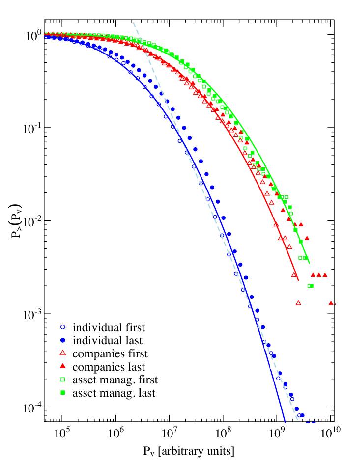
Figure 1: Reciprocal cumulative distribution function of the portfolio value $P_{v}$ for the three categories of clients at the time of their first (empty symbols) and last (filled symbols) transactions. Several models have been fitted to the data by Maximum Likelihood Estimation (MLE): the Student distribution (Pareto with plateau), the Weibull (stretched exponential), and the log-normal distribution. The best candidate, determined graphically and via bootstrapping the Kolmogorov Smirnov test [16] was found to be the log-normal distribution, which is the only one shown here for the sake of clarity. The dashed line in light blue results from a MLE fit to the tail of the individual traders with the Pareto distribution $p(x)\sim(x/x_{\min})^{-\gamma}$ (see section 3.1).

Numerous studies have been devoted to the analysis and modeling of wealth dynamics and distribution among a population (see [40] and references therein). The general picture is that in a population, a very large majority lies in the exponential part of the reciprocal cumulative distribution function, while the wealth of the richest people is Pareto-distributed, i.e., according to a power-law.

The account value of Swissquote traders is by definition the sum of all their assets (cash, stock, bonds, derivatives, funds, deposits), and denoted by $P_{v}$. In order to simplify our analysis, we compute $P_{v}$ once per day after US markets close and take this value as a proxy for the next day’s account value. Figure 1 displays this distribution computed at the time of the first and last transactions of the clients. Results are shown for the three main categories of clients. Maximum likelihood fits to the tail of the individual traders to the Pareto model $p(x)\sim(x/x_{\min})^{-\gamma}$ were performed using the BC_a bootstrap method of [21] and determining the parameter $x_{\min}$ by minimizing the Kolmogorov-Smirnov statistics as in [16]. Results are reported in table 1.

Table 1: Results of the fits of Pareto law $(x/x_{min})^{\gamma}$ to the account value $P_{v}$ of individuals.

individuals	$\gamma$	$x_{min}$
first transaction	$2.33\in[2.29,2.37]_{95}$	$2.30\cdot 10^{6}\in[1.99\cdot 10^{6},2.59\cdot 10^{6}]$
last transaction	$2.39\in[2.33,2.44]_{95}$	$3.73\cdot 10^{6}\in[3.15\cdot 10^{6},4.29\cdot 10^{6}]$

The values of $\gamma$ are in line with the wealth distribution of all major capitalistic countries (see [34] for a possible origin of Pareto exponents between 2.3 and 2.5). Thus the retail clients are most probably representative of the Swiss population. The account value distributions of companies and asset managers have no clear power-law tails, in agreement with the results of a recent model that suggests a log-normal distribution of mutual fund asset sizes [31]. Consequently, figure 1 also reports a fit of the data to log-normal distributions $\ln N(\mu,\sigma^{2})$, which approximate more faithfully $P_{>}(P_{v})$ than the Student and the Weibull distributions for the three categories of clients, except its extreme tail in the case of retail clients.

Table 2: Parameter values and 95% confidence intervals for the MLE fit of the account values to the log-normal distribution $\ln N(\mu,\sigma^{2})$. For each category of investors, the first and second row correspond to the account value at the time of the first, respectively the last transaction (see text). Note that portfolio values have been multiplied by an arbitrary number for confidentiality reasons. This only affects the value of $\mu$.

	$\mu$	$\sigma$
individuals	$13.94\pm 0.02$	$2.87\pm 0.01$
	$14.25\pm 0.02$	$2.01\pm 0.01$
companies	$16.0\pm 0.2$	$2.0\pm 0.1$
	$15.9\pm 0.2$	$2.4\pm 0.1$
asset managers	$16.7\pm 0.2$	$1.8\pm 0.1$
	$16.7\pm 0.2$	$2.0\pm 0.1$

3.2 Mean turnover

(a) Stocks

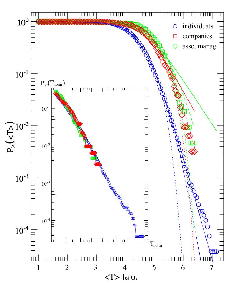
(b) Derivatives

Figure 2: Reverse cumulative distribution function of the mean turnover per transaction for the three categories of clients, and for both stock and derivative transactions. In the insets, the tail part of the RCDF of $\left\langle T_{norm}\right\rangle=\left\langle T\right\rangle/\mbox{mean}(\left\langle T\right\rangle)$. The solid curves are maximum likelihood fits to (1) for stocks and (2) for derivatives. The dotted lines are fits to the Weibull distribution and the dashed lines to the log-normal distribution.

The turnover of a single transaction $i$, denoted by $T_{i}$ is defined as the price paid times the volume of the transaction and does not include transaction fees. We have excluded the traders that have leveraged positions on stocks, hence $T_{i}\leq P_{v}$; more generally one wishes to determine how the average turnover of a given trader relates to his portfolio value. In passing, since $P(P_{v})$ has fat tails, the only way the distribution of $T$ can avoid having fat tails is if the typical turnover is proportional to $\log(P_{v})$. We denote by $\left<T\right>$ the mean turnover per transaction for a given client over the history of his activities.

Figure 2 reports its reciprocal cumulative distributions functions (RCDF) for stocks and derivatives for the three categories of clients; all RCDFs have a first plateau and then a fat tail. For stocks, the tails are not a pure power laws, but they are for derivatives. Indeed, fitting the RCDFs with Weibull, log-normal and Zipf-Mandelbrot distribution with an exponential cut-off, defined as

$$F_{>}^{(1)}(x)=\frac{c^{\gamma}e^{-\beta x}}{(c+x)^{\gamma}},$$ (1)

clearly shows that the latter is the only one that does not systematically underestimate the tail of the RCDF for stocks; estimated values of $\beta$ and $\gamma$ given in table 4.

The RCDFs related to the turnover of transactions on derivative products have clearer power-law tails for retail clients, which we fitted with a standard Zipf-Mandelbrot function, defined as

$$F_{>}^{(2)}(x)=\frac{c^{\gamma}}{(c+x)^{\gamma}}.$$ (2)

The parameters estimated are to be found in table 4; because of the power-law nature of this tail, fits with Weibull and log-normal distributions are not very good in the tails. While the decision process that allocates a budget to each type of product may be essentially the same, the buying power is larger for derivative products, which may explain the absence of a cut-off. Fits for companies and asset managers is very difficult and mostly non-conclusive because of unsufficient sample size; the good quality of the tail collapse (see inset) tends to indicate that the three distributions are identical, but we could not fit the RCDF of companies and asset managers with (2); as reported in figure 2b, log-normal distributions are adequate choices in these cases; since the quality of the fits are poor, we do not report the resulting parameters.

Table 3: Results of the maximum likelihood fit of $P_{>}(\left<T\right>)$ with (1) and (2) for the three categories of clients. The 95% confidence intervals reported in smaller character are computed by the biased-corrected accelerated (BC_a) bootstrap method of [21].

	Stocks (1)		Derivatives (2)
	$\gamma$	$\beta\cdot 10^{-6}$	$\gamma$
individuals	1.97	0.98	1.98
	[1.83,2.10]	[0.46,1.5]	[1.91,2.15]
companies	1.29	1.66	-
	[1.52,1.89]	[0.44,2.3]
asset managers	1.93	0.91	-
	[1.47,2.93]	[-7.8,4.5]

3.3 Mean turnover vs account value

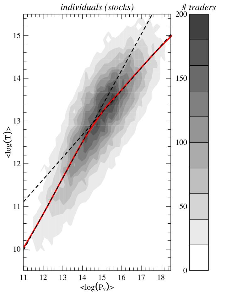
Figure 3: Density plot of the average $\log T$ vs the average $\log P_{v}$, robust non-parametric fit (red line), and linear fits (dashed lines)

The relationship between $\left<T\right>$ vs $\left<P_{v}\right>$ is important as it dictates what fraction of their investable wealth the traders exchange in markets. We first produce a scatter plot of $\left<\log T\right>$ vs $\left<\log P_{v}\right>$ (figure 4). In a log-log scale plot, it shows a cloud of points that is roughly increasing. A density plot is however clearer for retail clients as there are many more points (figure 3).

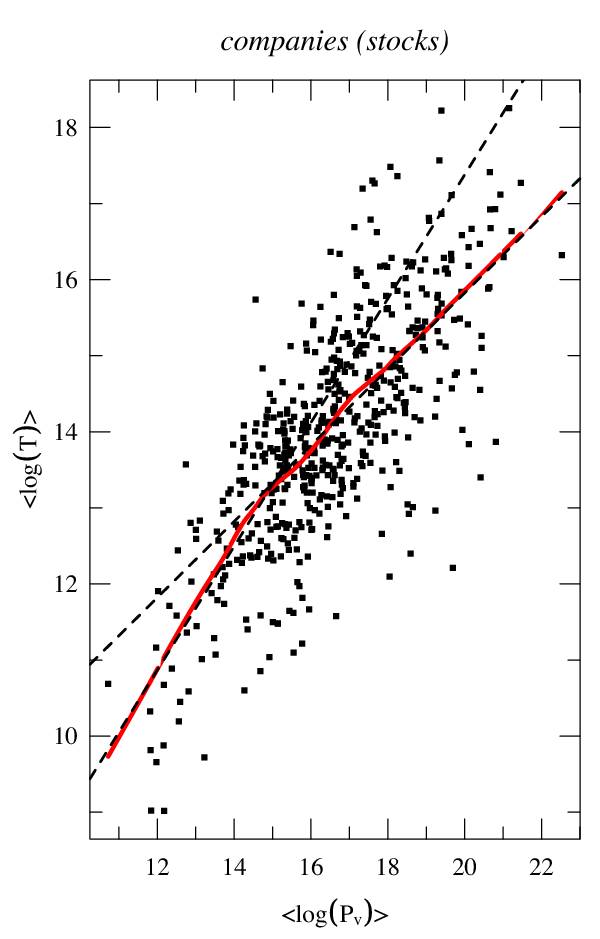
(a)

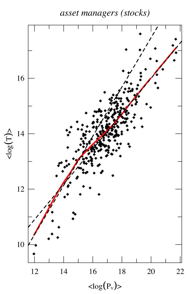
(b)

Figure 4: Density plot of the average $\log T$ vs the average $\log P_{v}$, robust non-parametric fit (red line), and linear fits (dashed lines)

These plots make it clear that there are simple relationships between $\log T$ and $\log P_{v}$. A robust non-parametric regression method [17] reveals a double linear relationship between $\left\langle\log T\right\rangle$ and $\left\langle\log P_{v}\right\rangle$ for all three categories of investors (see figures 4 and 3):

$$\left\langle\log T\right\rangle=\beta_{x}\left\langle\log P_{v}\right\rangle+a_{x}$$ (3)

where $x=1$ when $\left\langle\log P_{v}\right\rangle<\Theta_{1}$ and $x=2$ when $\left\langle\log P_{v}\right\rangle>\Theta_{2}$. Fitted values with confidence intervals are reported in table 5.

Table 5: Parameter values and 95% confidence intervals for the double linear model (4). For each category of investors, the first and second row correspond respectively to $\left\langle\log P_{v}\right\rangle\leq\Theta_{1}$ an $\left\langle\log P_{v}\right\rangle\geq\Theta_{2}$. For confidentiality reasons, we have multiplied $P_{v}$ and $T$ by a random number. This only affects the true values of $a_{x}$ and $\Theta$ in the table.

	$\beta_{x}$	$a_{x}$	$\xi$	$\Theta$	$R^{2}$
individuals	$0.84\pm 0.02$	$0.73\pm 1.25$	0.71	14	0.52
	$0.54\pm 0.01$	$5.07\pm 0.15$	0.77	14.5	0.40
companies	$0.81\pm 0.13$	$1.12\pm 8.17$	0.88	15.5	0.47
	$0.50\pm 0.07$	$5.82\pm 1.65$	1.00	15.6	0.33
asset managers	$0.89\pm 0.20$	$-0.31\pm 0.76$	0.62	15.5	0.52
	$0.63\pm 0.08$	$3.28\pm 5.78$	0.62	16.5	0.46

This result is remarkable in two respects: (i) the double linear relation, not obvious to the naked eye, separates investors into two groups (ii) the ranges of values where the transition occurs is very similar across the three categories of traders.

The relationships above only applies to averages over all the agents. This means that there are some intrinsic quantities that make all the agents deviate from this average line. Detailed examination of the regression residuals show that the latter are for the most part (i.e. more than 95%) normally distributed with constant standard deviations $\xi_{x}$ and that the residuals deviating from the normal distributions are not fat-tailed. This directly suggests the simple relation for individual traders

$$T^{i}=e^{a_{x}+\delta^{i}a_{x}}(P_{v}^{i})^{\beta_{x}}\leq e^{\Theta_{x}}$$ (4)

where $T^{i}$ and $P_{v}^{i}$ are respectively the turnover and portfolio value of investor $i$, and $\delta^{i}a_{x}$ are i.i.d. $N(0,\xi_{x}^{2})$ idiosyncratic variations independent from $P_{v}$ that mirror the heterogeneity of the agents. As we shall see, portfolio optimization with heterogeneous parameters yields this precise relationship.

3.4 Turnover rescaled by account value

Let us now measure the typical fraction of wealth exchanged in a single transaction, defined as $Q=\left<\frac{T}{P_{v}}\right>$. Since the inverse of this ratio is an indirect (and imperfect) proxy of the number $N$ of assets that a trader owns, it also indicates how well diversified his investments are, hence, it can be viewed a simple proxy of the risk profiles of the agents.

3.4.1 data

Figure 5 shows that the distributions look exponential to a naked eye for about 90% of the individuals and nearly 80% of the companies, while that of the asset managers is rapidly more complex that a simple exponential. We derive exact relationships for this quantity in subsection 3.4.2 that show that these distributions are in fact not exponential but log-normal.

The resulting picture is that only a small fraction of customers trade a large fraction of their wealth on average. Interestingly, these figures show a clear difference between the three categories of clients. As discussed above, figure 5 roughly reflects the risk profile of the different types of customers: less than 10% of asset managers trade on average more than 20% of their clients’ capital in a single transaction; this rises to 30% for companies, and 45% for retail clients. Note however that despite the fact that the account values of companies and asset managers are comparable, companies tend to have a $Q$ closer to that of the individuals; this suggests either that companies hold a smaller $N$ than asset managers for the same account value, or that asset managers tend to make smaller adjustments to the quantities of assets.

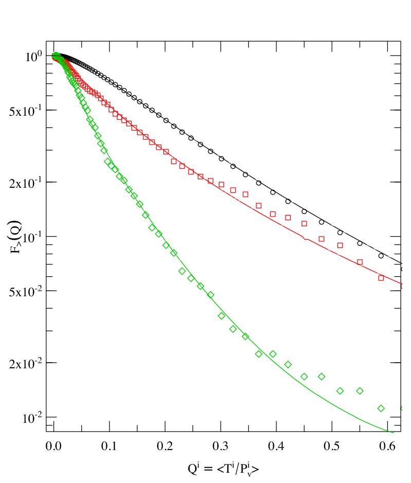
(a)

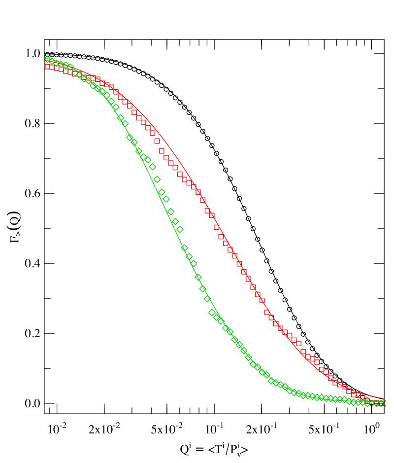
(b)

Figure 5: Reverse cumulative distribution function of $Q=\left<\frac{T}{P_{v}}\right>$, the mean ratio of the turnover over the portfolio value for individual traders (black), companies (red) and asset managers (green). Left plot is in lin-log scale and right plot is in log-lin scale. Solid lines come from theoretical predictions of section 3.4.2.

3.4.2 theory

Since we know the distributions of $T$, $P_{v}$ and their relationship, we are in a position to derive analytical expressions for $Q^{i}=\left\langle\frac{T(t)}{P_{v}(t)}\right\rangle$ of investor $i$. The distribution of $Q$ across the population of on-line investors can be easily found using (4) and the distribution of $P_{v}$. Let $P_{T,P_{v}}(t,p_{v})$ denote the joint distribution of $T$ and $P_{v}$:

$$P_{Q=\frac{T}{P_{v}}}(q)=\int_{0}^{\infty}p_{v}P_{T,P_{v}}(qp_{v},p_{v})\,dp_{v}=\int_{0}^{\infty}p_{v}P_{T|P_{v}}(qp_{v}|p_{v})P_{P_{v}}(p_{v})\,dp_{v}.$$ (5)

Let us now assume for the sake of clarity that $T=e^{a+\delta a}P_{v}^{\beta}$. Given $P_{v}$, the turnover $T$ follows a log-normal distribution with mean $\log p_{v}+a$ and variance $\xi^{2}$. Substituting $P_{T|P_{v}}(t|p_{v})=\ln N\left(\log p_{v}+a,\xi^{2}\right)$ in (5) leads after some simplifications to

$$P_{Q}(q)=\int_{0}^{\infty}\frac{1}{\sqrt{2\pi\xi^{2}}q}\exp\left(-\frac{\left(\log(qp_{v}^{1-\beta})-a\right)^{2}}{2\xi^{2}}\right)P_{P_{v}}(p_{v})\,dp_{v},$$ (6)

and

$$F_{Q}(q)=\int_{0}^{q}P_{Q}(x)\,dx=\int_{0}^{\infty}\frac{1}{2}\mbox{erfc}\left(\frac{a-\log(qp_{v}^{1-\beta})}{\sqrt{2}\xi}\right)P_{P_{v}}(p_{v})\,dp_{v},$$ (7)

where $\mbox{erfc}(x)=\frac{2}{\sqrt{\pi}}\int_{x}^{\infty}e^{-y^{2}}\,dy$ is the complementary error function. As expected, when $\beta=0$ (i.e. $T$ and $P_{v}$ are independent), we recover the product of the two marginal distributions. On the other hand, when $\beta=1$, i.e., when $T$ is proportional to $P_{v}$, $P_{Q}(q)=\ln N\left(a,\xi^{2}\right)$, which is the distribution of the factor $e^{a+\delta a}$. For other values of $\beta$ the functions $P_{Q}$ and $F_{Q}$ cannot be determined analytically unless $P_{P_{v}}$ takes a particular form as shown below. However, the moments of $P_{Q}(q)$ can be arranged in a simpler form:

$$E(q^{n})=\int_{0}^{\infty}q^{n}P_{Q}(q)dq=e^{na+\frac{1}{2}n^{2}\xi^{2}}\int_{0}^{\infty}\frac{1}{p_{v}^{n(1-\beta)}}P_{P_{v}}(p_{v})\,dp_{v},$$ (8)

that is, the (log-normal) moments of $T/P_{v}$ times an integral term smaller or equal to $1$ (because in practice $P_{P_{v}}(p_{v})>1$). Hence, the relation $E(q^{n})\leq e^{na+\frac{1}{2}n^{2}\xi^{2}}$ with equality when $\beta=1$ holds for any distribution of the account value $P_{v}$.

In section 3.1, we have shown that the distribution of $P_{v}$ is well-approximated by a log-normal distribution. This particular choice of distribution makes the previous integrals analytically tractable. Indeed, with $P_{P_{v}}=\ln N(\mu,\sigma^{2})$ straight integration of (6) leads to $P_{Q}=\ln N(M,S^{2})$, where $M=a-(1-\beta)\mu$ and $S^{2}=\xi^{2}+(1-\beta)^{2}\sigma^{2}$. This simple result has some practical interest: given the distribution parameters and the coupling factor $\beta$, one can draw realistic $q$ factors for agent-based modeling as $Q=e^{M+SX}$, where $X$ is $\mathcal{N}(0,1)$ distributed. Furthermore, in the next section, we show how the value of $\beta$ may be inferred from the transaction cost structure, which decreases the number of parameters to four.

Figure 5 confirms the validity of the above theoretical results, once expanded to the case of a bi-linear relation between $T$ and $P_{v}$. It is noteworthy that the continuous lines are no fits on empirical $q$ factors, but use instead the results of the separate fits on the turnover and account distributions.

4 The influence of transaction costs on trading behavior: optimal mean-variance portfolios

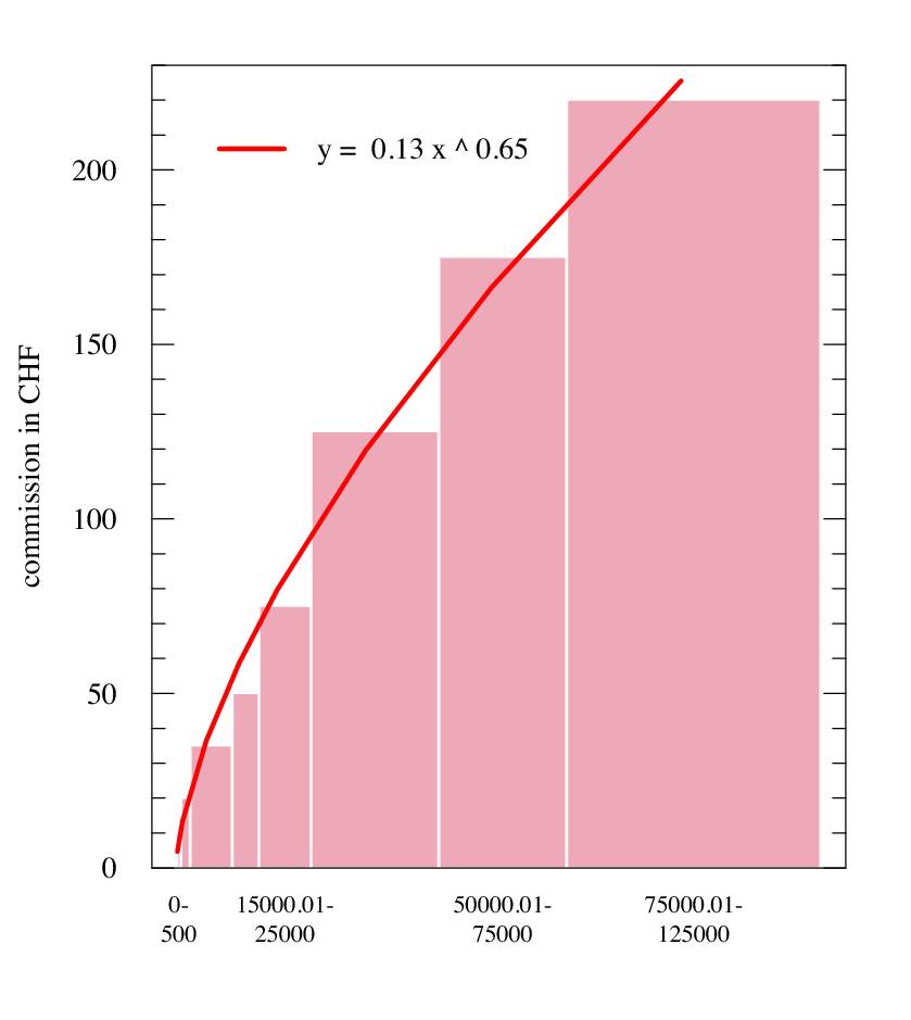
Figure 6: Swissquote fee curve for the Swiss stock market. Commissions based on a sliding scale of costs are common practice in the world of on-line finance. The red line results from a non-linear fit to equation 10. Parameter values are $C=0.13\in[0.05,0.5]_{95}$ and $\delta=0.63\in[0.5,0.74]_{95}$, where the 95% confidence intervals are obtained from the BC_a bootstrap method of [21].

Apart from risk profiles, education, and typical wealth, the differences in the turnover as a function of wealth observed above between the three populations of traders may also lie in the difference of their actual transaction cost structure. Swissquote current standard structure for the Swiss market (its shape is very similar for European and US markets) is shown in figure 6; it is a piece-wise constant, non-linear looking function. Fitting all segments to equation 10 gives $\delta=0.63\in[0.5,0.74]_{95}$. The fee structure of most brokers is not set in stone and can be negotiated. A frequent request is to have a flat fee, i.e. a fixed cost per transaction corresponding to a constant function. Since quite clearly the negotiation power of large clients or of clients that carry out many transactions is more important, asset managers are more likely to obtain a more favorable fee structure than basic retail clients.

Since buying some shares of an asset is the result of unconscious or calculated portfolio construction process, one first needs a theoretical reference point with which to compare the population characteristics as measured in the previous subsection. In other words, we shall use results from portfolio optimization theory with non-linear transaction cost functions to understand the results of the previous subsection.

Quite curiously, all analytical papers in the literature on optimal portfolios either neglect transaction costs or assume constant or linear transaction cost structures; non-linear structures are tackled numerically; thus, we incorporate the specific non-linear transaction cost structure faced by the traders under investigation in the classic one-shot portfolio optimization problem studied by Brennan [8], who restricted its discussion to fees proportional to the number of securities, in other words, a flat fee per transaction.

Building optimal mean-variance stock portfolios consists for a given agent in selecting which stock to invest in and in what proportion by maximizing the expected portfolio growth, usually called return, while trying to reduce the resulting a priori risk. One cost function that corresponds to such requirements is

$$L_{\lambda}(R)=\lambda E(R)\mbox{-Var}(R),$$ (9)

where $R$ is the stochastic return of the portfolio over the investment horizon (e.g., one month, one year) and $\lambda$ tunes the trade-off between risk and return; as such, it can be interpreted as a measure of an investor’s attitude towards risk: the larger $\lambda$ , the more risk-adverse the investor.

The return of the portfolio can be decomposed into contributions from risky assets (stocks, derivatives, etc.), the interests of the amount kept in cash, and the total relative cost of broker commission, which we denote as $R=R^{risky}+R^{cash}-R^{cost}$. Mathematically,

• $R^{risky}=\Sigma_{i=1}^{N}x_{i}R_{i}$, where $R_{i}$ is the return of stock $i$ over this horizon, $x_{i}$ is the fraction of the total wealth invested in this stock, and $N$ is the total number of investable assets; we shall denote the total fraction of wealth invested in risky assets by $x=\sum_{i=1}^{N}x_{i}$;

• $R^{cash}=(1-x)r$, where $r$ is the interest rate;

• $R^{cost}=\frac{\sum_{i=1}^{N}F(x_{i}P_{v})}{P_{v}}(1+r)$, where $F(x)$ is the amount charged by a broker to exchange an amount $x$ of cash into shares or vice-versa.

The focus of this section is to derive explicit relationships between $F$, the number of assets to hold in a portfolio, and the account value $P_{v}$. Whereas previous works only considered special cases for $F$ that are not compatible with the fees structure of Swissquote, we need to introduce a cost function that can accommodate all the standard broker commission schemes. The two extreme cases are i) flat-fee per transaction, i.e., a fixed cost that does not depend on the amount exchanged ii) a proportional scheme, possibly with a maximum fee. Swissquote’s standard scheme stands in between and is well approximated by a power-law with a maximum fee $F_{max}$. We hence choose

$$F(x_{i}P_{v})=\min\left(C(x_{i}P_{v})^{\delta},F_{max}\right),$$ (10)

where $\delta$ interpolates between a flat-fee ($\delta=0$), as in [8], and a proportional scheme ($\delta=1$) via a power-law, and $C$ is a constant.

Following the well-known one-factor model of Sharpe [32], we assume that the return of asset $i$ follows the global market’s return $R_{M}$ with an idiosyncratic proportionality factor $\beta_{i}$. More specifically,

$$R_{i}=\beta_{i}(R_{M}-r)+r+\varepsilon_{i},$$ (11)

where $\varepsilon_{i}$ is an uncorrelated white noise $E(\varepsilon_{i})=E(\varepsilon_{i}\varepsilon_{j})=E(R_{M}\varepsilon_{i})=0.$ This equation means that the systematic idiosyncratic part of $R_{i}$ only applies to the return above the risk-free interest rate, also called market risk premium.

This completely specifies the functional $L_{\lambda}$. Returning to (9), one first computes the expectation and variance of the portfolio return:

$$E(R) = \sum_{i=1}^{N}x_{i}E(R_{i})+(1-x)r-\frac{\sum_{i=1}^{N}F(x_{i}P_{v})}{P_{v}}(1+r),$$ (12)

$$= (E(R_{M})-r)\sum_{i=1}^{N}x_{i}\beta_{i}+r-\frac{(1+r)C}{P_{v}^{1-\delta}}\sum_{i=1}^{N}x_{i}^{\delta},$$

and

$$\mbox{Var}(R) = \mbox{Var}(R^{risky})$$ (13)

$$= \mbox{Var}(R_{M})\sum_{i=1}^{N}(x_{i}\beta_{i})^{2}+\sum_{i=1}^{N}x_{i}^{2}\mbox{Var}(\varepsilon_{i}).$$

Note that, since here the risk-free rate is non-random, the portfolio variance is independent of both the risk-free investment and broker commission; this does not hold for the expected return.

In principle, the functional $L$ depends on $N$, the number of assets in the portfolio, $\lambda$ the risk parameter, and $x_{i}$ the fraction of account value to invest in risky product $i$. Assuming that $x_{i}$ is constant for all $i$ (i.e. equally-weighted allocation), we are left with only three parameters since $x_{i}=x/N$. Thus, from the optimization of the resulting functional one can obtain a relationship between any two of these parameters. We are mostly interested in $N$ as a function of $x$.

4.1 Non-linear relationship between account value and number of assets

We will first assume that agents seek the optimal fraction of their account value $x^{*}$ to invest in $N$ securities—$N$ being known—given the risk free rate $r$ and broker commission $F(x_{i}W)$. The optimal solution is simply obtained by setting $x_{i}=x/N$ in (12) and (13), and by equating to zero the derivative of (9) with respect to $x$. This leads to the following transcendental equation for $x^{*}$:

$$x^{*}=\frac{\lambda}{2}\frac{\bar{\beta}(E(R_{M})-r)-\delta(1+r)C(\frac{N}{x^{*}P_{v}})^{1-\delta}}{\bar{\beta}^{2}\mbox{Var}(R_{M})+\frac{1}{N}\overline{\mbox{Var}}(\varepsilon)},$$ (14)

where $\bar{\beta}=\frac{1}{N}\sum_{i=1}^{N}\beta_{i}$ and $\overline{\mbox{Var}}(\varepsilon)=\frac{1}{N}\sum_{i=1}^{N}\mbox{Var}(\varepsilon_{i})$ is the mean idiosyncratic volatility. Provided the investor risk tolerance $\lambda$ has been reliably estimated, which is usually a complex task [39], and that Sharpe model is adequate, (14) can be used directly in a real-world portfolio optimization problem. The $\beta_{i}$ and $\varepsilon_{i}$ are then obtained by regressing the returns of all the stocks with (11); the optimal solution is expected to be reliable in the absence of significant residual correlations between $\varepsilon_{i}$ and $\varepsilon_{j}$. In the more common situation where $\lambda$ is unknown, one can derive a second equation for the optimal number of securities under the assumption that portfolios are sufficiently homogeneous, or that the investment horizon is long enough so as to have $\bar{\beta}$ and $\overline{\mbox{Var}}(\varepsilon)$ independent from $N$. As shown in figure 7, $\bar{\beta}$ on the US stock market is persistently close to one for various time horizons and values of $N$, consistently with the homogeneous assumption. Taking a few technical precautions into account ([8]), the differentiation of the Lagrangian (9) with respect to $N$ leads to

$$\lambda=\frac{\overline{\mbox{Var}}(\varepsilon)P_{v}^{1-\delta}}{(1-\delta)C(1+r)\left(\frac{N^{*}}{x}\right)^{2-\delta}},$$ (15)

where it is assumed that $\delta<1$ since for $\delta=1$ the optimum investment does not depend on $N$ through the cost function. According to (15), the agent risk tolerance increases with their account value $P_{v}$, in agreement with various survey studies on the risk tolerance of actual investors (see the literature review of [38]). Using (14) and (15) to get rid of $\lambda$, we obtain

$$N^{2-\delta}\left(1+\frac{\delta}{1-\delta}\frac{K}{N}\right)=K\frac{\bar{\beta}(E(R_{M})-r)}{(1-\delta)C(1+r)}\left(xP_{v}\right)^{1-\delta},$$ (16)

where $K$ is the ratio of residual risk to market risk defined as

$$K=2\left(\frac{\bar{\beta}^{2}\mbox{Var}(R_{M})}{\overline{\mbox{Var}}(\varepsilon)}+\frac{1}{N}\right)^{-1}\underset{N\gg 1}{\approx}2\frac{\overline{\mbox{Var}}(\varepsilon)}{\bar{\beta}^{2}\mbox{Var}(R_{M})}.$$ (17)

Given the desired level of systematic risk $x$, (16) can be solved for $N$ numerically in an actual portfolio optimization. Further insight is gained by considering the high diversification limit $N\gg 1$, which yields $1+\frac{\delta}{1-\delta}\frac{K}{N}\approx 1$ in (16) and thus

$$N=\left(K\frac{\bar{\beta}(E(R_{M})-r)}{(1-\delta)C(1+r)}\right)^{\frac{1}{2-\delta}}\left(xP_{v}\right)^{\frac{1-\delta}{2-\delta}},$$ (18)

where $K$ is given by the right-hand side of (17). The latter equation generalizes [8] to the case of a varying cost impact represented here by the parameter $\delta$ (i.e. the result of [8] is recovered by setting $\delta=0$ and $\beta_{i}=1$ in (18)). These results can be further generalized to non-equally weighted portfolios by differentiating (9) with respect to $x_{i}$ and assuming again an homogeneous condition for the $\beta_{i}$s.

In essence, (18) says that the number of securities held in an equally-weighted mean-variance portfolio with Sharpe-like returns is related to the amount invested as

$$\log(N)=\frac{1-\delta}{2-\delta}\log(xP_{v})+\mbox{$\kappa$}$$ (19)

in the high diversification limit, where $\kappa$ is the pre-factor of $\left(xP_{v}\right)^{\frac{1-\delta}{2-\delta}}$ in (18). The last equation gives $N$ as a function of $P_{v}$ for a predefined $x$ in the optimal portfolio. The heterogeneity of the traders, beyond their account value, is not apparent yet, but may occur both in $x$ and $\kappa$: first each trader may have his own preference regarding the fraction of this account to invest in risky assets, $x$; therefore one should replace $x$ by $x^{i}$; next, $\kappa$ includes both a term related to transaction costs, which does vary from trader to trader, and some measures and expectation of market returns and variance; each trader may have his own perception or way of measuring them, hence $\kappa$ should also be replaced by $\kappa^{i}$. Finally, both terms can be merged in the same constant term $\zeta^{i}=\frac{1-\delta}{2-\delta}\log(x^{i})+\kappa^{i}$. This explains how the heterogeneity of the traders is the cause of fluctuations in the kind of relationships we are interested in.

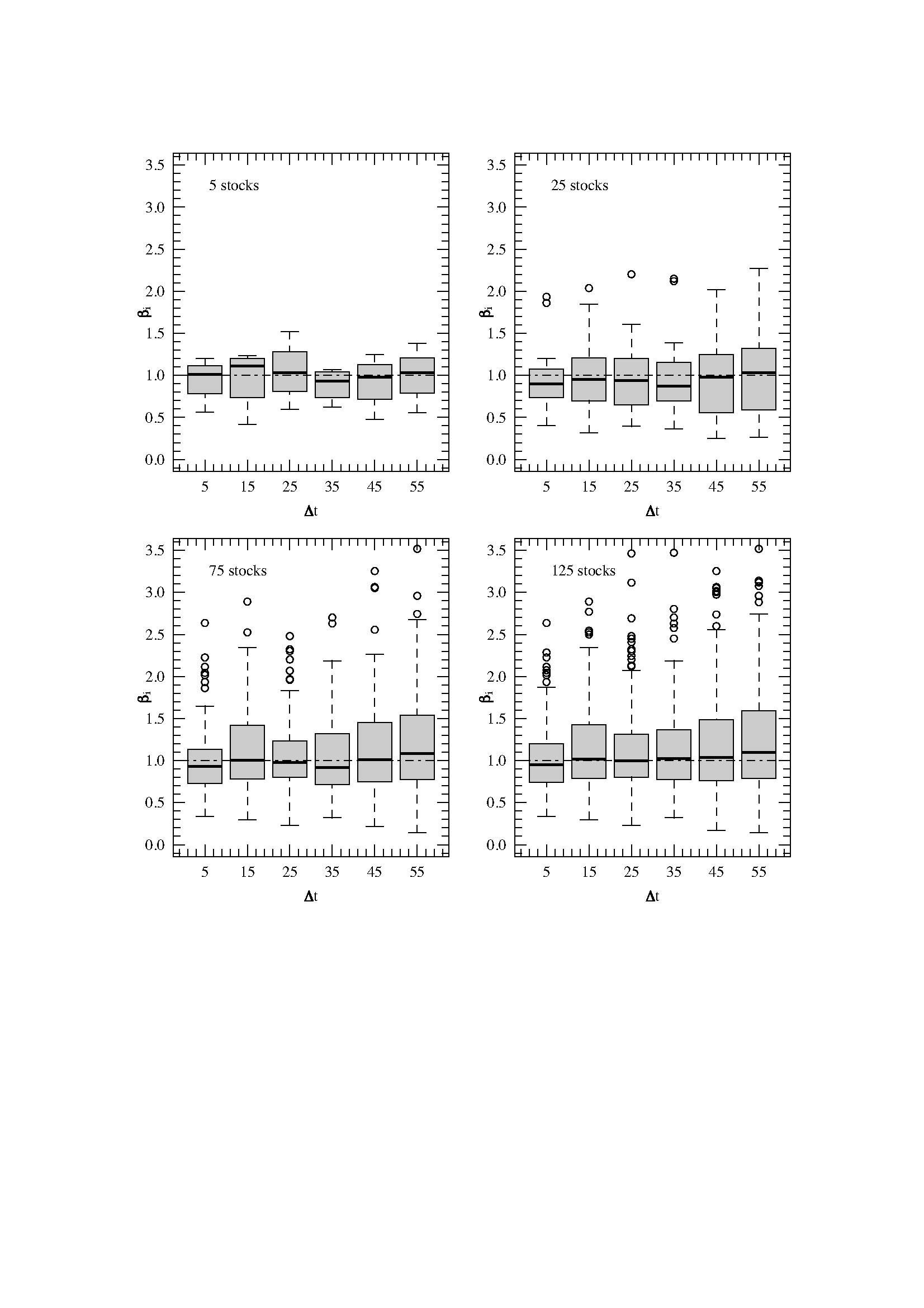
Figure 7: Box-plot of empirical $\beta$s obtained from the regression of several US stocks on the S&P500. The observation period covers 2001 to 2008 and returns are computed on various time horizons $\Delta t$ (in days). Results show that $\bar{\beta}=\frac{1}{N}\sum_{i=1}^{N}\beta_{i}\approx 1$ for all values of $\Delta t$ and (even small) $N$, consistently with the homogeneous assumption of section 4.1.

5 Turnover, number of assets and account value

The result above only links $N$ with $P_{v}$, but one also wishes to obtain relationships that involve the turnover per transaction, $T$. Whereas in section 3, we have characterized the turnover of any transaction, the results of section 4 rest on the assumption that the agents build their portfolio by selecting a group of assets and stick to them over a period of time. This, obviously, does not include the possibility of speculating by a series of buy and sell trades on even a single asset, nor portfolio rebalancing which consists in adjusting the relative proportions of some assets. We thus have to find a way to differentiate between portfolio building, rebalancing and speculation. Here, we shall focus on portfolio building in order to test and link the results of section 4 to those of section 3.

We have found a simple effective method that can separate portfolio-building transactions from the other ones: we assume that the transactions of trader $i$ that correspond to the building of his portfolio are restricted the first transaction of assets not traded previously; sell orders are ignored, since Swissquote clients cannot short sell easily. In other words, if trader $i$ owns some shares of assets A, B, and C and then buys some shares of asset D, the corresponding transaction is deemed to contribute to his portfolio building process; the set of such transactions is denoted by $\Phi_{i}$, while the full set of transactions is denoted by $\Omega_{i}$. Any subsequent transaction of shares of assets A, B, C, or D are left out of $\Phi_{i}$. The number of different assets that trader $i$ owns is supposed to be $N_{i}\simeq|\Phi_{i}|$ where $|X|$ is the cardinal of set $X$; this approach assumes that a trader always owns shares in all the assets ever traded; surprisingly, this is by large the most common case. We shall drop the index $i$ from now on.

Let us now focus on $T_{\Phi}=\sum_{k\in\Phi}T_{k}$, the total turnover that helped building his portfolio. We should first check how it is related to the total portfolio value $P_{v}$. Let us define $\left\langle P_{v}\right\rangle_{\Phi}$, the account value of a trader averaged at the times at which he trades a new asset.Plotting $\log\left\langle P_{v}\right\rangle_{\Phi}$ against $\log T_{\Phi}$ gives a cloudy relationship, as usual, but the fitting it with $\log\left\langle P_{v}\right\rangle_{\Phi}=\chi\log T_{\Phi}$ gives $\chi=1.03\pm 0.02$ for individuals, $\chi=0.99\pm 0.02$ for asset managers and $\chi=1.00\pm 0.01$ for companies with an adjusted $R^{2}=0.99$ in all cases. This relationship trivially holds for the traders who buy all their assets at once, as assumed in the portfolio model. The traders who do not lie on this line either hold positions in cash (in which case this line is a lower bound), or do not build their portfolio in a single day: they pile up positions in derivative products or stocks whose price fluctuations are the origin of the devations from the line. But the fact that the slope is close to 1 means that the average fluctuation is zero, hence, that on average trades do not make money from the positions taken on new stocks. The consequence of this is that $\log P_{v}$ can be replaced by $\log T_{\Phi}$ in (19), thus, setting $x=1$,

$$\log N=\frac{1-\delta}{2-\delta}\log T_{\Phi}+\mbox{$\kappa$}$$ (20)

The $x=1$ assumption is in fact quite reasonable: most Swissquote traders do not use their trading account as savings accounts and are fully invested; we do not know what amount they keep on their other bank accounts.

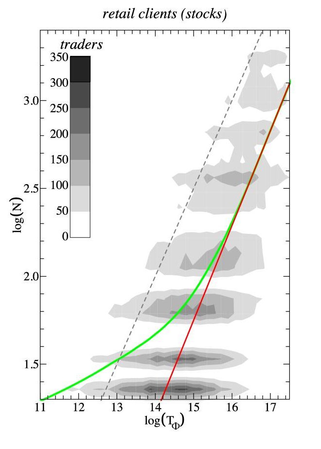
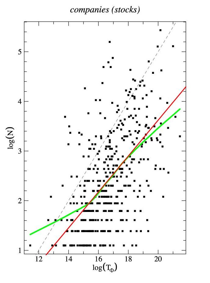
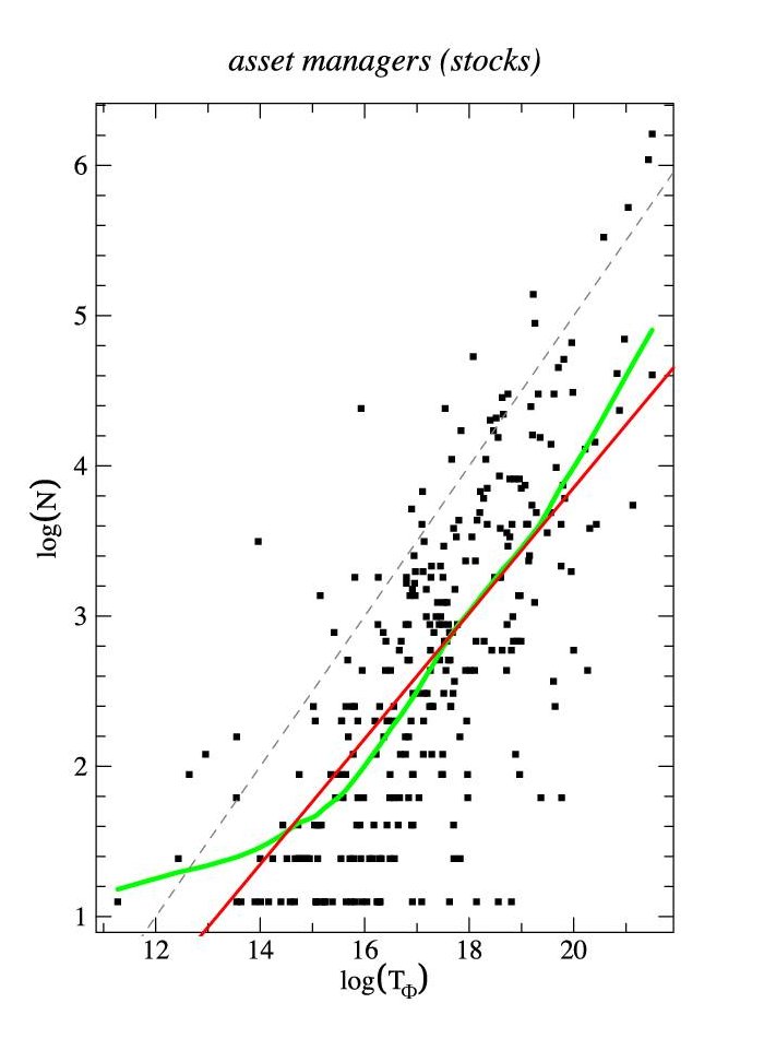
Figure 8: Turnover of transactions contributing to the building of a portfolio $T_{\Phi}$ versus the number $N$ of assets held by a given trader at the time of the transaction. Green lines: non-parametric fit; red lines: fits of the linear part of the non-parametric fit. From left to right: companies, asset managers, and individuals.

Table 6: Slope $\alpha$ linking $\log T_{\Phi}$ and $\log N$ for the three trader categories.

	individuals	companies	asset managers
$\alpha$	$0.52\pm 0.02$	$0.36\pm 0.14$	$0.44\pm 0.13$
$\log T_{\Phi}\in$	$[16,19]$	$[17,19.8]$	$[15.8,18]$

Table 7: Results of the double linear regression of $\log\left\langle T\right\rangle_{\Phi}$ versus $\log\left\langle P_{v}\right\rangle_{\Phi}$. For each category of investors, the first and second row correspond respectively to $\log\left\langle P_{v}\right\rangle_{\Phi}\leq\Theta_{1}$ an $\log\left\langle P_{v}\right\rangle_{\Phi}\geq\Theta_{2}$, where $\Theta_{1,2}$ have been determined graphically using the non-parametric method of [17] as in section 3.3. Parameters are as in the double linear model (4). For confidentiality reasons, we have multiplied $P_{v}$ and $T$ by a random number, which only affects the true values of $\Theta_{1,2}$ and of the ordinate $a_{x}$.

	$\beta_{x}$	$a_{x}$	$\xi$	$\Theta$	$R^{2}$
individuals	$0.85\pm 0.02$	$0.71\pm 0.16$	0.65	14.5	0.59
	$0.51\pm 0.01$	$5.62\pm 0.17$	0.76	15	0.31
companies	$0.83\pm 0.17$	$1.03\pm 2.47$	0.86	15.5	0.42
	$0.62\pm 0.14$	$3.99\pm 2.55$	0.93	17	0.32
asset managers	$0.84\pm 0.25$	$0.45\pm 3.77$	0.79	15.95	0.50
	$0.73\pm 0.17$	$1.72\pm 3.23$	0.72	18	0.41

A robust non-parametric fit does reveal a linear relationship between $\log N$ and $\log T_{\Phi}$ in a given region $(N,T_{\Phi})\in\Gamma$ (figure 8). In this region, we have

$$\log N=\alpha\log T_{\Phi}+\beta,$$ (21)

which gives

$$\alpha=\frac{1-\delta}{2-\delta}.$$ (22)

We still need to link $\left\langle T\right\rangle_{\Phi}$ and $\left\langle P_{v}\right\rangle_{\Phi}^{\beta}$. While section 3 showed that the unconditional averages lead to $\left\langle T\right\rangle\sim\left\langle P_{v}\right\rangle^{\beta}$, one also finds that $\left\langle T\right\rangle_{\Phi}\sim\left\langle P_{v}\right\rangle_{\Phi}^{\beta}$. Therefore, one can write

$$\log\left\langle T\right\rangle_{\Phi}=\beta\log\left\langle P_{v}\right\rangle_{\Phi}+\mbox{cst}.$$ (23)

Thus, one is finally rewarded with the missing link

$$\beta=\frac{1}{2-\delta},$$ (24)

which directly involves the transaction cost structure in the relationship between turnover and portfolio value, as argued in section 3. This relationship allows us to close the loop as we are now able to relate directly the exponents linking $T$, $N$, and $P_{v}$. Going back to section 3, one understands that the existence of a bi-linear relationship between log-turnover and log-account value, i.e., of two values of $\beta$ for each of the three categories of clients, is linked to two values of $\delta$: a flat flee structure or the disregard for transaction costs leads to $\beta=\frac{1}{2}$, while proportional fees ($\delta=1$) give $\beta=1$.

Let us finally discuss the empirical values of $\alpha$, $\beta$, and $\delta$ against their theoretical counterparts, which is summarized in table 8.

1. Small values of $T_{\Phi}$: it was impossible to measure $\alpha$ in that case since the non-parametric fit shows a non-linear relationship in the log-log plot for retail clients, which we trust more since they have many many more points than the graphs for the two other categories of clients. But it may not make sense to expect a linear relationship since such a relationship is only expected for $N$ large enough ($N\geq 10$ in practice) and a small $T_{\Phi}$ is related to a small $N$. Thus we can only test $\beta=1/(2-\delta)$. The reported value of $\beta$ is consistent accross all the clients. Retail clients have a larger $\delta_{eff}=2-\frac{1}{\beta}$ that the estimated $\delta_{SQ}$. Since the shape of the fee structure is discontinuous, the values of these exponents can hardly be expected to match. However, fitting the whole curve structure may be problematic in this context: indeed, the traders with a typical small value of $T_{\Phi}$ see a more linear relationship in the region of small transaction value that when considering the whole curve; for instance, removing the two largest segments from the fee structure yields $\delta_{SQ}^{\prime}=0.74\in[0.43,0.79]$, which is not far of $\delta_{eff}$.

2. Large values of $T_{\Phi}$: the relationships between all the exponents are verified for the three categories of clients. While not very impressive for companies and asset managers, this result is much stronger in the case of retail clients since the relative uncertainties associated with each measured exponent are small (1-2%). The value of $\beta_{retail}$ is of particular interest as it corresponds $\delta_{eff}=0$, or equivalently, to a flat fee structure. Going back to the fees structure of Swissquote, one finds that that the transition happens when the relative transaction cost falls below some threshold (we cannot give its precise value for confidentiality reasons; it is smaller than 1%). A possible explanation is that either some traders with a high enough average turnover have a flat-fee agreement with Swissquote and that the rest of them simply act as if they were not able to take correctly into account transaction costs. Since not all traders have a flat-fee aggrement, one must conclude that some traders have indeed some problems estimating small relative fees and simply disregard them. The reported value of $\beta$ for companies and asset managers is larger that $\beta_{retail}$, but it is more likely than not that the small sample size is responsible for this discrepancy, since these two categories of clients have a greater propensity to negociate a flat-fee structure.

3. Transition between the two regimes: the transitions between the standard Swissquote and an effective flat-fee structure happens occur at the same average value of $T$ for the three categories of traders (idem for $T_{\Phi}$). Since there is no automatic switching between fee structures at Swissquote for any predefined value of transaction value, one is lead to conclude that this transition has behavioural origins, which is also responsible for the value at which the transition takes place which, in passing, corresponds to the end of the plateau of the RCDF of $P_{v}$ in the case of retail clients ($e^{15}\simeq 3.27\cdot 10^{6}$). As a consequence, it is likely that the traders tend to either neglect or consider as constant transaction fees smaller than some threshold when they build their portfolio.

Table 8: Table summarising the empirical and theoretical relationships between $\alpha$, $\beta$, and $\delta$.

small $T_{\phi}$	individuals	companies	asset managers
$\beta$	$0.85\pm 0.02$	$0.83\pm 0.17$	$0.84\pm 0.25$
$\log T_{\Phi}<$	14.5	17	18
$\delta_{eff}=2-\frac{1}{\beta}$	$0.82\pm 0.02$	$0.80\pm 0.20$	$0.81\pm 0.30$
$\delta_{SQ}$	$0.63\in[0.50,0.74]$	$0.63\in[0.50,0.74]$	$0.63\in[0.50,0.74]$
$\delta_{SQ}^{\prime}$	$0.74\in[0.43,0.79]$	$0.74\in[0.43,0.79]$	$0.74\in[0.43,0.79]$
$\tilde{\beta}=\frac{1}{2-\delta_{SQ}}$	$0.73\in[0.66,0.74]$	$0.73\in[0.66,0.74]$	$0.73\in[0.66,0.74]$

large $T_{\phi}$	individuals	companies	asset managers
$\beta$	$0.51\pm 0.01$	$0.62\pm 0.14$	$0.73\pm 0.17$
$\log T_{\Phi}>$	15	17	18
$\delta_{eff}=2-\frac{1}{\beta}$	$0.04\pm 0.02$	$0.39\pm 0.23$	$0.63\pm 0.23$
$\alpha_{eff}=\frac{1-\delta_{eff}}{2-\delta_{eff}}$	$0.49\pm 0.01$	$0.38\pm 0.09$	$0.27\pm 0.08$
$\alpha$	$0.52\pm 0.02$	$0.36\pm 0.14$	$0.44\pm 0.13$
$\log T_{\Phi}\in$	$[16,19]$	$[17,19.8]$	$[15.8,18]$

6 Discussion and outlook

We have been able to determine empirically a bilinear relationship between the average log-turnover and the average log-account value and have argued that it comes from the transaction fee structure of the broker and its perception by the agents. A theoretical derivation of optimal simple one-shot mean-variance portfolios with non-linear transaction costs predicted relationships between turnover, number of different asset in the portfolio and log-account values that could be verified empirically. This means that the populations of traders do take correctly on average, i.e. collectively, the transaction costs into account and act $collectively$ as mean-variance equally-weighted portfolio optimizers. This is not to say that each trader is a mean-variance optimizer, but that the population taken as a whole behaves as such—with differences across populations, as discussed in the previous section. This to be related to findings of Kirman’s famous work on demand and offer average curves in Marseille’s fish market [24] and more generally as what has become known as the wisdom of the crowds (see [35] for an easy-to-read account).

The fact that the turnover depends in a non-linear way on the account value implies that linking the exponents of the distributions of transaction volume, buying power of large players in financial markets, and price return is more complex that previously thought [23]. It has also implications for agent-based models, which from now on must take into account the fact that the real traders do invest into a number of assets that depends non-linearly on their wealth.

Future research will address the relationship between account value and trading frequency, which is of utmost importance to understand if the many small trades of small investors have a comparable influence on financial market than those of institutional investors. This will give an understanding of whom provides liquidity and what all the non-linear relationships found above mean in this respect. This is also crucial in agent-based models, in which one often imposes such relationship by hand, arbitrarily; reversely, one will be able to validate evolutionary mechanisms of agent-based model according to the relationship between trading frequency, turnover, number of assets and account value they achieve in their steady state.

References

- [1] Alfarano, S., and Lux, T. A minimal noise traders model with realistic time series properties. In Long memory in Economics. Springer, Berlin, 2003.
- [2] Arthur, B. W. Inductive reasoning and bounded rationality: the El Farol problem. Am. Econ. Rev. 84 (1994), 406–411.
- [3] Barber, B. M., Lee, Y.-T., Liu, Y.-J., and Odea, T. Do individual day traders make money? evidence from taiwan.
- [4] Bauer, R., Cosemans, M., and Eichholtz, P. The performance and persistence of individual investors: Rational agents or tulip maniacs? http://papers.ssrn.com/sol3/papers.cfm?abstract_id=965810.
- [5] Bouchaud, J.-P., Farmer, J. D., and Lillo, F. How markets slowly digest changes in supply and demand. arXiv:0809.0822.
- [6] Bouchaud, J.-P., Giardina, I., and Mézard, M. On a universal mechanism for long ranged volatility correlations. Quant. Fin. 1 (2001), 212. cond-mat/0012156.
- [7] Bouchaud, J.-P., and Potters, M. Theory of Financial Risks. Cambridge University Press, Cambridge, 2000.
- [8] Brennan, M. The optimal number of securities in a risky asset portfolio when there are fixed costs of transacting: Theory and some empirical results. The Journal of Financial and Quantitative Analysis 10, 3 (1975), 483–496.
- [9] Brock, W. A., and Hommes, C. H. A rational route to randomness. Econometrica 65 (1997), 1059–1095.
- [10] Caldarelli, G., Marsili, M., and Zhang, Y.-C. A prototype model of stock exchange. Europhysics Letters 50 (1997), 479–484.
- [11] Challet, D., Chessa, A., Marsili, M., and Zhang, Y.-C. From minority games to real markets. Quant. Fin. 1 (2000), 168. cond-mat/0011042.
- [12] Challet, D., and Marsili, M. Criticality and finite size effects in a realistic model of stock market. Phys. Rev. E 68 (2003), 036132.
- [13] Challet, D., Marsili, M., and Zhang, Y.-C. Minority Games. Oxford University Press, Oxford, 2005.
- [14] Challet, D., and Stinchcombe, R. Non-constant rates and over-diffusive prices in a simple model of limit order markets. Quant. Fin. 3 (2001), 155.
- [15] Challet, D., and Zhang, Y.-C. Emergence of cooperation and organization in an evolutionary game. Physica A 246 (1997), 407. adap-org/9708006.
- [16] Clauset, A., Shalizi, C. R., and Newman, M. E. J. Power-law distributions in empirical data. SCIAM Review 51, 661–703.
- [17] Cleveland, W. S., and Devlin, S. J. Locally weighted regression: An approach to regression analysis by local fitting. Journal of the American Statistical Association 83, 403 (1988), 596–610.
- [18] Cont, R., and Bouchaud, J.-P. Herd behaviour and aggregate fluctuation in financial markets. Macroecon. Dyn. 4 (2000), 170.
- [19] Dacorogna, M. M., Gencay, R., Müller, U. A., Olsen, R. B., and Pictet, O. V. An Introduction to High-Frequency Finance. Academic Press, London, 2001.
- [20] Dea, S., Gondhib, N. R., Manglac, V., and Pochirajud, B. Success/failure of past trades and trading behavior of investors.
- [21] Efron, B., and Tibshirani, R. J. An Introduction to the Bootstrap. Chapman & Hall, New York, 1993.
- [22] Farmer, J. D., and Lillo, F. On the origin of power law tails in price fluctuations. Quant. Fin. 4 (2003), 7. cond-mat/0309416.
- [23] Gabaix, X., Gopikrishnan, P., Plerou, V., and Stanley, H. A theory of power-law distributions in financial market fluctuations. Nature 423 (2003), 267.
- [24] Härdle, W., and Kirman, A. Nonclassical demand: A model-free examination of price-quantity relations in the Marseille fish market. Journal of Econometrics 67, 1 (1995), 227–257.
- [25] Jefferies, P., Hart, M., Hui, P., and Johnson, N. From market games to real-world markets. Eur. Phys. J. B 20 (2001), 493–502. cond-mat/0008387.
- [26] Lillo, F. Limit order placement as an utility maximization problem and the origin of power law distribution of limit order prices. Eur. Phys. J. B 55, 4 (2007), 453–459. physics/0612016.
- [27] Lux, T., and Marchesi, M. Scaling and criticality in a stochastic multi-agent model of a financial market. Nature 397 (1999), 498–500.
- [28] Mantegna, R., and Stanley, H. G. Introduction to Econophysics. Cambridge University Press, 2000.
- [29] Maslov, S., Zhang, Y.-C., and Marsili, M. Dynamical optimization theory of a diversified portfolio. Physica A 253 (1998), 403–418.
- [30] Raffaelli, G., and Marsili, M. Dynamic instability in a phenomenological model of correlated assets. J. Stat. Mech. (2006). doi:10.1088/1742-5468/2006/08/L08001.
- [31] Schwarzkopf, Y., Farmer, J., and Set, I. Time Evolution of the Mutual Fund Size Distribution.
- [32] Sharpe, W. Capital asset prices: A theory of market equilibrium under conditions of risk. The Journal of Finance 19, 3 (1964), 425–442.
- [33] Slanina, F., and Zhang, Y.-C. Dynamical spin-glass-like behavior in an evolutionary game. Physica A 289 (2001), 290–300.
- [34] Solomon, S., and Richmond, P. Power laws of wealth, market order volumes and market returns. Physica A: Statistical Mechanics and its Applications 299, 1-2 (2001), 188–197.
- [35] Surowiecki, J. The wisdom of crowds. Anchor Books, New York, NY, 2005.
- [36] Thurner, S., Farmer, J., and Geanakoplos, J. Leverage causes fat tails and clustered volatility. Preprint.
- [37] Vaglica, G., Lillo, F., Moro, E., and Mantegna, R. Scaling laws of strategic behavior and size heterogeneity in agent dynamics. Physical Review E 77, 3 (2008), 36110.
- [38] Van de Venter, G., and Michayluk, D. A longitudinal study of financial risk tolerance. Tech. rep., 2009. http://www.fma.org/Reno/Papers/Longitudinal_Financial_Risk_Tolerance.pd%f.
- [39] Veld, C., and Veld-Merkoulova, Y. V. The risk perceptions of individual investors. Journal of Economic Psychology 29, 2 (April 2008), 226–252.
- [40] Yakovenko, V. Econophysics, statistical mechanics approach to. Encyclopedia of Complexity and System Science, Springer http://refworks. springer (2007).