Curvaton reheating in logamediate inflationary model

Abstract

In a logamediate inflationary universe model we introduce the curvaton field in order to bring this inflationary model to an end. In this approach we determine the reheating temperature. We also outline some interesting constraints on the parameters that describe our models. Thus, we give the parameter space in this scenario.

I Introduction

It is well known that one of the most exciting ideas of contemporary physics is to explain the origin of the observed structures in our Universe. It is believed that inflation R1 can provide an elegant mechanism to explain the large-scale structure, as a result of quantum fluctuations in the early expanding Universe, predicting that small density perturbations are likely to be generated in the very early universe with a nearly scale-free spectrum R2 . This prediction has been supported by early observational data, specifically in the detection of temperature fluctuations in the cosmic microwave background (CMB) by the COBE satellite R4 . In this epoch, the predictions of inflation have been detected in the specific pattern of anisotropies imprinted in the full sky map of the CMB, as reported, for instance, by the WMAP mission R5 . On the other hand, an inflationary-type expansion also sources a back-ground of primordial gravitational waves R6 , whose effects still remain undetectable. Forthcoming observations, such as the PLANCK R7 or LISA R8 missions, may measure effects of relic gravitational waves and offer new trends for gravitational physics in the near future.

The condition for inflation to occur is that the inflaton field slow-roll near the top of the potential for sufficiently long time, so that the vacuum energy drives the inflationary expansion of the Universe. Many models of inflation have been proposed R9 ; R10 , based on single field or multifield potentials. Also, they have been constructed in various theoretical schemes. We distinguish those introduced by Barrow R11 where the scale factor $a(t)$ as the asymptotic property that ordinary differential equations of the form $\ddot{a}=P(a,t)/Q(a,t)$, as $t\rightarrow\infty$ with polynomials $P$ and $Q$, brings specific different solutions from which we singularize those named logamediate inflationary solution. This solution has the interesting property that the ratio of tensor to scalar perturbations is small and the power spectrum can be either red or blue tilted, according to the values of the parameters appearing in the model R12 .

The main motivation to study logamediate inflationary universe models becomes from the form of the field potential that appear in this kind of models, i.e. $V(\phi)\propto\,\phi^{\alpha}\;\exp[-\beta\,\phi^{\gamma}]$. This potential includes exponential potential ($\alpha=0$) that appears in Kaluza-Klein theories, as well as in supergravity, and in superstring models (see Ref.P1 ). Also, it includes power-law potentials ($\beta=0$), with models based on dynamical supersymmetry breaking which motivates potentials of the type, $V(\phi)\propto\phi^{-\alpha}$ P2 . We also find this sort of potentials in models motivated by higher-dimensional theories, scalar-tensor theories, and supergravity corrections P3 . In particular, it was used in Ref.P4 for studying inflation with a background dilaton field, and scaling behavior and other attractorlike solutions were studied in Ref.P5 . On the other hand, this potential was used in dark energy models, driving the observed acceleration of the Universe at the present epoch P6 .

In Ref.A2 was considered the behavior of the parameters $\gamma$ and $\alpha$ in all regions of the parameter space. When $0\leq\gamma\leq 1$, inflation is generic at late times, for all values of $\alpha$. For the cases, when $\gamma>1$ and $\alpha\neq 0$, the models are noninflationary. When $\gamma<0$ and $\alpha\geq 0$, inflation comes at early times. For $\gamma<0$ and $\alpha<0$, inflation occurs at late times and the inflationary behavior is regulated by the specific value of $\alpha$. For $\gamma>1$ and $\alpha=0$ the quasi-de Sitter scenario is manifest at early times, but this is not a characteristic as $t\rightarrow\infty$, where all models are noninflationary. For the case $\gamma>1$ and $\alpha\neq 0$, these models can never inflate. In particular, if $\gamma=0$, the solutions present polynomial-chaotic or intermediate inflationary behavior depending upon the sign of $\alpha$, and for the special case when $\alpha=0$ the de Sitter solution is obtained. The power-law solutions occur for $\gamma=1$ and $\alpha=0$ and if $\alpha\neq 0$ the behavior will asymptote to the power-law solution at large times $t$. If $0<\gamma<1$ the scale factor is proportional to $\exp(\ln^{(2-\gamma)/\gamma})$ as $t\rightarrow\infty$.

One of the drawbacks of this model rests on the impossibility to bring inflation to an ends. In fact, at the end of inflation the energy density of the universe is locked up in a combination of kinetic and potential energies of the scalar field, which drives inflation R9 . One path to defrost the universe after inflation is known as reheating R14 . During reheating, most of the matter and radiation of the universe are created usually via the decay of the inflaton field leading to a creation of particles of different kinds, while the temperature grows in many orders of magnitude. It is at this point where the universe matches the Big-Bang model. In this process is the particular interest in in the quantity known as the reheating temperature, $T_{rh}$. The reheating temperature is related to the temperature of the Universe when the radiation epoch begins.

The oscillations of the scalar inflaton field are an essential part for the standard mechanism of reheating. However, there are some models where the inflaton potential does not have a minimum and the scalar field does not oscillate. Here, the standard mechanism of reheating does not work R15 . These models are known in the literature like nonoscillating (NO) models R16 ; R17 . The NO models correspond to runaway fields such as module fields in string theory which are potentially useful for inflation model-building because they presents flat directions which survive the famous $\eta$-problem of inflation R18 . This problem is related to the fact that between the inflationary plateau and the quintessential tail there is a difference of over a 100 orders of magnitude.

The first mechanism of reheating in this kind of model was the gravitational particle production R20 , but this mechanism is quite inefficient, since it may lead to certain cosmological problems R21 ; R22 . An alternative mechanism of reheating in NO models is the instant preheating, which introduce an interaction between the inflaton scalar field an another scalar field R16 . Another possibility for reheating in NO models is the introduction of the curvaton field, $\sigma$, R23 , which has recently received a lot of attention in the literature R24 ; R25 . The curvaton approach is an interesting new proposal for explaining the observed large-scale adiabatic density perturbations in the context of inflation. Here, the hypothesis is such that the adiabatic density perturbation originates from the -”curvaton field”- and not from the inflaton field. In this scenario, the adiabatic density perturbation is generated only after inflation, from an initial condition which corresponds to a purely isocurvature perturbation R26 . Following, Ref.M1 (see, also Ref.M2 ) we adopt the ”curvaton hypothesis”, where the inflaton perturbation is taken to be less than 1$\%$ of the observed value. Using the COBE normalization at the pivot scale, we can set an upper bound for the power spectrum of inflation, where $P_{\zeta_{\phi}}^{1/2}\lesssim\,0.01\,P_{\zeta}^{1/2}\simeq 5\times\,10^{-7}$. Here, $P_{\zeta_{\phi}}^{1/2}$ and $P_{\zeta}^{1/2}$ are the power spectrum of the inflaton field and curvaton field, respectively. On the other hand, generally inflationary models suggest that inflation took place at energy comparable to that of grand unification, where the energy scale is approximately $V_{*}^{1/4}\approx 10^{15-16}$ GeV , where $V_{*}$ is the effective potential associated with the inflaton field evaluated when the cosmological scales exit the horizon M3 . In the context of string landscape supersymmetry sets the value of $V_{*}$ at scales typically much less than the grand unified scale. One way to liberate inflation from the constraint given by $V_{*}^{1/4}\approx 10^{15-16}$ GeV is to consider that the curvature perturbations generated during inflation are due to quantum fluctuations of the curvaton field, in which case $V_{*}^{1/4}\approx 10^{15-16}$ GeV turns into an upper bound M1 . It is assumed that the curvaton field does not influence the dynamics of the inflaton field, but becomes important after inflation has ended, when it imprints its curvature perturbation onto the universe R23 . Under this hypothesis, it is possible to diminish this constraint substantially M4 . However, we should note that, one can have cases in which the fluctuations generated by both, the inflaton and a curvatonlike field are relevant M5 ; M6 .

In the framework of logamediate inflationary universe models we would like to introduce the curvaton field as a mechanism to bring logamediate inflation to an end. Therefore, the main aim of this paper is to carry out the curvaton field into the logamediate inflationary scenario and see what consequences we may derive. The outline of the paper goes as follow: in Sec. II we give a brief description of the logamediate inflationary scenario. In Sec III the curvaton field is described in the kinetic epoch. Section IV describes the curvaton decay after its domination. Section V describe the decay of the curvaton field before it dominates. Section VI studies the consequences of the gravitational waves. At the end, Sec. VII includes our conclusions.

II Logamediate inflation Model

In order to introduce the logamediate inflationary universe model we start with the corresponding field equations that must satisfy the scalar field in a flat Friedmann-Robertson-Walker (FRW) background

$$3\;H^{2}=\frac{\dot{\phi}^{2}}{2}+V(\phi),$$ (1)

and

$$\ddot{\phi}+3H\dot{\phi}=-\frac{\partial V(\phi)}{\partial\phi},$$ (2)

where $H\equiv\dot{a}/a$ is the Hubble factor, $a=a(t)$ is the scale factor. Here, $\phi$ is the standard inflaton field and $V(\phi)$ its associated effective scalar potential, the dots denote derivative with respect to the cosmological time $t$, and we shall use units such that $8\pi G=8\pi/m_{p}^{2}=c=\hbar=1$,   $m_{p}$ being the Planck mass.

The main assumption in the logamediate inflationary universe model is that the scale factor $a(t)$ expands by means of the asymptotic form R11 ; R12

$$a(t)=\exp[\,A\,(\ln t)^{\lambda}],$$ (3)

with $t>1$. Here $A>0$, and $\lambda>1$ are constants. The Hubble parameter as a function of the cosmological times $t$ becomes

$$H=\frac{\dot{a}}{a}=\frac{A\,\lambda(\ln\,t)^{\lambda-1}}{t},$$ (4)

and since $A\,\lambda>0$ we get expanding universe. Note that when $\lambda=1$ this model reduces the well known power-law inflation, $a\propto t^{p}$, where $p=A$ with $A>1$. From Eqs. (1-3), we have $\dot{H}=-\dot{\phi}^{2}/2$ and the scalar field $\phi(t)$ result

$$\phi=\phi_{0}+\gamma\,(A\lambda)^{1/2}\,(\ln t)^{\frac{1}{\gamma}},$$ (5)

where $\gamma=\frac{2}{\lambda+1}$.

Assuming the set of slow-roll conditions, i.e., $\dot{\phi}^{2}\ll V(\phi)$ and $\ddot{\phi}\ll 3H\dot{\phi}$, and setting $\phi_{0}=0$, without loss of generality, the scalar potential can be written as R12

$$V(\phi)=V_{0}\,\phi^{\alpha}\,\exp[-\beta\,\phi^{\gamma}].$$ (6)

Here, the parameters $\alpha$ and $\beta$ are defined by $\alpha=\frac{4(\lambda-1)}{(\lambda+1)}$ and $\beta=2\left[\frac{(\lambda+1)}{(2\sqrt{2}(A\lambda)^{1/2})}\right]^{2/(\lambda+1)}$, respectively. Furthermore, we have defined

$$V_{0}=\frac{3}{2}(A\lambda)^{2}\,\beta^{2(\lambda-1)}.$$ (7)

Note that this kind of potential does not present a minimum for large values of the field $\phi$. This potential was originally studied by Barrow A1 (see also Ref.A2 ), where it was shown that the condition $\gamma=2/(\lambda+1)\leq 1$ was needed for inflation to occurs at large values of $\phi$.

The Hubble factor as a function of the inflaton field, $\phi$, becomes

$$H(\phi)=H_{0}\,\phi^{\frac{\alpha}{2}}\,\exp\left[-\beta\,\phi^{\gamma}/2\right],$$ (8)

where $H_{0}=\sqrt{V_{0}/3}$.

The slow-roll parameters, $\varepsilon$ and $\eta$, are defined by $\varepsilon=\frac{V^{\prime 2}}{2V^{2}}$ and $\eta=V^{\prime\prime}/V$, respectively. Here the prime denotes derivative with respect to the inflaton field $\phi$. In the present case they read

$$\varepsilon=\frac{1}{2\phi^{2}}\left(\alpha-\beta\,\gamma\phi^{\gamma}\right)^{2},\;\;\;\mbox{and}\;\;\;\eta=-\frac{1}{\phi^{2}}\left[\alpha+\beta\,\gamma\,(\gamma-1)\,\phi^{\gamma}-\frac{1}{2}(\alpha-\beta\,\gamma\,\phi^{\gamma})^{2}\right],$$ (9)

and its ratio results in $\frac{\varepsilon}{\eta}=\left[1-2\frac{\alpha+\beta\,\gamma\,(\gamma-1)\,\phi^{\gamma}}{(\alpha-\beta\,\gamma\,\phi^{\gamma})^{2}}\right]^{-1}$.

Note that, the parameters $\varepsilon$ and $\eta$ diverges when the scalar field $\phi\rightarrow 0$. Also, $\varepsilon$ is always larger than $\eta$ since $\beta$ is positive ($A>0$ and $\lambda>1$), then $\varepsilon$ reaches unity before $\eta$ does. In this way, we may establish that the end of inflation is governed by the condition $\varepsilon=1$. From the condition $\varepsilon=1$ we can distinguish two possible solutions for the scalar field, at the end of inflation: $\phi_{e}=\frac{\alpha}{\sqrt{2}}$ for the value of $\alpha>\beta\,\gamma\,\phi^{\gamma}$ and $\phi_{e}=\left(\frac{\beta^{2}\,\gamma^{2}}{2}\right)^{\frac{1}{2(1-\gamma)}}$, for $\alpha<\beta\,\gamma\,\phi^{\gamma}$. From now on, the subscript $e$ will be used to denote the end of the inflationary period. The maximum of the potential occurs when the parameter $\varepsilon=0$ ($\partial V/\partial\phi=0$) and the value of the scalar field in this maximum of the potential is $\phi_{i}=(\alpha/(\beta\gamma))^{1/\gamma}$. In the following, we study our inflationary scenario and the reheating of the Universe for values of the scalar field, such that $\phi_{i}\leq\phi$. Then, we are taking $\phi_{e}=\left(\frac{\beta^{2}\,\gamma^{2}}{2}\right)^{\frac{1}{2(1-\gamma)}}$, because with this choice it is possible to get a continuous transition from the inflationary age to the kinetic phase.

III The curvaton field

When inflation has finished, the model enters to the -”kinetic epoch”- (or -”kination”-, for simplicity) Ag1 . In this epoch, the term $\displaystyle\frac{\partial V(\phi)}{\partial\phi}$ is negligible compared to the friction term $3H\dot{\phi}$ in the field Eq. (2). Hereafter, with the subscript (or superscript) -”k”- we label different quantities at the beginning of this epoch. The kinetic epoch does not occur immediately after inflation; there may exist a middle epoch where the potential force is negligible with respect to the friction term Ag2 . During the kination epoch we have that $\dot{\phi}^{2}/2>V(\phi)$ which could be seen as a stiff fluid since the relation between the pressure $P_{\phi}$ and the energy density $\rho_{\phi}$, corresponds to the relation $P_{\phi}\simeq\rho_{\phi}$.

During the kinetic epoch we have $3\;H^{2}\,=\rho_{\phi}\simeq\frac{\dot{\phi}^{2}}{2}$ and $\ddot{\phi}+3H\dot{\phi}=0$, where the latter equation could be solved and gives $\dot{\phi}=\dot{\phi}_{k}\left({\frac{a_{k}}{a}}\right)^{3}$. This expression yields

$$\rho_{\phi}(a)=\rho_{\phi}^{k}\left(\frac{a_{k}}{a}\right)^{6},$$ (10)

and the Hubble parameter becomes

$$H(a)=H=H_{k}\left(\frac{a_{k}}{a}\right)^{3},$$ (11)

where $H_{k}^{2}=\frac{\rho_{\phi}^{k}}{3}\simeq\frac{\dot{\phi}_{k}^{2}}{6}$ is the value of the Hubble parameter at the beginning of the kination.

We now study the dynamics of the curvaton field, $\sigma$, through different stages. We consider that the curvaton field obeys the Klein-Gordon equation and, for simplicity, we assume that its scalar potential associated with this field is given by $U(\sigma)=\frac{m^{2}\sigma^{2}}{2}$, where $m$ is the curvaton mass. This study allows us to find some constraints on the parameters and thus, to have a viable curvaton scenario.

First, we assume that the energy density $\rho_{\phi}$, associated with the inflaton field, is the dominant component when it is compared with the curvaton energy density, $\rho_{\sigma}$, i.e., $\rho_{\phi}\gg\rho_{\sigma}$. In the next stage, the curvaton field oscillates around the minimum of the effective potential $U(\sigma)$. Its energy density evolves as a nonrelativistic matter and, during the kinetic epoch, the universe remains inflaton-dominated. Finally, the last stage corresponds to the decay of the curvaton field into radiation and then the standard big-bang cosmology is recovered.

In the inflationary regime it is supposed that the curvaton field mass $m$ satisfied the condition $m\ll H_{e}$, and its dynamics is described in detail in Refs.dimo ; postma ; cdch . During inflation, the curvaton would roll down its potential until its kinetic energy is depleted by the exponential expansion and only then, i.e. only after its kinetic energy has almost vanished, it becomes frozen and assumes roughly a constant value, i.e., $\sigma_{*}\approx\sigma_{e}$. The subscript ”$*$” here refers to the epoch when the cosmological scales exit the horizon.

During the kinetic epoch the Hubble parameter decreases so that its value is comparable with the curvaton mass, and the curvaton mass is of the order of Hubble parameter, i.e., $H\simeq m$. Then from Eq. (11), we obtain

$$\frac{m}{H_{k}}=\left(\frac{a_{k}}{a_{m}}\right)^{3},$$ (12)

where the subscript ${}^{\prime}m^{\prime}$ stands for quantities evaluated at the time when the curvaton mass, $m$, is of the order of $H$.

In order to prevent a period of curvaton-driven inflation the universe must still be dominated by the inflaton field, i.e., $\rho_{\phi}|_{a_{m}}=\rho_{\phi}^{m}\gg\rho_{\sigma}$. Over the inflation period the effective potential does not change substantially, because it is reasonable to suppose that $\rho_{\phi}^{m}\gg\rho_{\sigma}\sim U(\sigma_{e})\simeq\,U(\sigma_{*})$. The quoted inequality allows us to find a constraint on the values of the curvaton field $\sigma_{*}$ at the moment when $H\simeq m$, since

$$\frac{m^{2}\sigma_{*}^{2}}{2\rho_{\phi}^{m}}=\frac{\sigma_{*}^{2}}{6}\ll\,\,1\,,$$ (13)

or equivalently $\sigma_{*}^{2}\ll 6$.

Now, at the end of inflation the ratio between the potential energies results

$$\frac{U_{e}}{V_{e}}=\frac{m^{2}\sigma_{*}^{2}}{6H_{e}^{2}}\ll\,\frac{m^{2}}{H_{e}^{2}},$$ (14)

here, we have used Eq.(13).

Since the curvaton energy becomes subdominant at the end of inflation, i.e., $V_{e}\gg U_{e}$, then the curvaton mass should obey the constraint $m^{2}\ll H_{e}^{2}$, and using the relations $H^{2}_{e}=V_{e}/3$, Eq.(14) and $\phi_{e}=(\beta^{2}\gamma^{2}/2)^{1/2(1-\gamma)}$, we get

$$m^{2}\ll\frac{V_{0}}{3}\,\left(\frac{2}{\beta^{2}\gamma^{2}}\right)^{\frac{\alpha}{2(\gamma-1)}}\,\exp\left[-\beta\,\left(\frac{2}{\beta^{2}\gamma^{2}}\right)^{\frac{\gamma}{2(\gamma-1)}}\right].$$ (15)

After the curvaton field becomes effectively massive, its energy decays as a nonrelativistic matter in the form $\rho_{\sigma}=\frac{m^{2}\sigma_{*}^{2}}{2}\left(\frac{a_{m}}{a}\right)^{3}$. In the following, we will study the decay of the curvaton field in two possible different scenarios.

IV Curvaton Decay After Domination

For the first scenario, when the curvaton field comes to dominate the cosmic expansion i.e., $\rho_{\sigma}>\rho_{\phi}$, there must be a moment in which the inflaton and curvaton energy densities match. We are going to assume that this happens when $a=a_{eq}$. Then, from Eqs.(10) and (11), and bearing in mind that $\rho_{\sigma}\propto\,a^{-3}$, we get

$$\left.\frac{\rho_{\sigma}}{\rho_{\phi}}\right|_{a=a_{eq}}=\frac{m^{2}\sigma_{*}^{2}}{2}\frac{a_{m}^{3}\;a_{eq}^{3}}{a_{k}^{6}\;\rho_{\phi}^{k}}=\frac{m^{2}\sigma_{*}^{2}a_{m}^{3}a_{eq}^{3}}{6\;H_{k}^{2}\;a_{k}^{6}}=1,$$ (16)

where we have used the relation $3\,H_{k}^{2}=\rho_{\phi}^{k}$ together with $H_{k}\left(\frac{a_{k}}{a_{eq}}\right)^{3}=\frac{m\sigma_{*}^{2}}{6}$ and Eq.(12).

In terms of the curvaton parameters, the Hubble parameter, $H(a_{eq})=H_{eq}$ can be rewritten as

$$H_{eq} = H_{k}\left(\frac{a_{k}}{a_{eq}}\right)^{3}=\frac{m\;\sigma_{*}^{2}}{6},$$ (17)

where we have considered Eqs.(11), (12) and (16).

When the curvaton decays after domination we require that the following condition is fulfilled, $\rho_{\sigma}>\rho_{\phi}$, in addition to the decay parameter $\Gamma_{\sigma}<H_{eq}$. Since the decay parameter $\Gamma_{\sigma}$ is constrained by nucleosynthesis, it is required that the curvaton field decays before nucleosynthesis, which means $H_{nucl}\sim 10^{-40}<\Gamma_{\sigma}$. Hence, the constraint upon the decay parameter is

$$10^{-40}<\Gamma_{\sigma}<\frac{m\;\sigma_{*}^{2}}{6}.$$ (18)

The curvaton approach is potentially valuable in the search of physical constraints on the parameters appearing in the logamediate expanding model by studying the scalar perturbations related to the curvaton field $\sigma$. During the time in which the fluctuations are inside the horizon, they obey the same differential equation of the inflaton fluctuations. We may conclude that they acquire the amplitude $\delta\sigma_{*}\simeq H_{*}/2\pi$. On the other hand, outside of the horizon, the fluctuations obey the same differential equation like the unperturbed curvaton field and then, we expect that they remain constant over inflation. The spectrum of the Bardeen parameter, $P_{\zeta}$, whose observed value is $P_{\zeta}\simeq 2.4\times 10^{-9}$ WMAP3 , allows us to determine the value of the curvaton field, $\sigma$, evaluated at the epoch when the cosmological scales exit the horizon. This becomes in terms of the parameters $A$ and $\beta$. At the time when the decay of the curvaton field occurs the parameter $P_{\zeta}$ results to in ref1u

$$P_{\zeta}\simeq\frac{H_{*}^{2}}{9\pi^{2}\sigma_{*}^{2}}\simeq\frac{1}{9\pi^{2}\sigma_{*}^{2}}\,H_{0}^{2}\left[B\,N_{*}+\,\phi_{e}^{\lambda\gamma}\right]^{\frac{2(\lambda-1)}{\lambda}}\,\exp\left[-\beta\left(B\,N_{*}+\phi_{e}^{\lambda\gamma}\right)^{1/\lambda}\right],$$ (19)

where $B=A^{-1}\;\left(A\lambda\gamma^{2}\right)^{\lambda/(\lambda+1)}$. Here, the number of e-folds, $N_{*}$, is determined by $N_{*}=\int_{t_{*}}^{t_{e}}H(t^{\prime})dt^{\prime}$. After a rather involved lengthy but straightforward computation we get

$$N_{*}=A\left[\frac{(\lambda+1)}{2(A\lambda)^{1/2}}\right]^{\frac{2\lambda}{\lambda+1}}\left(\phi_{*}^{\frac{2\lambda}{\lambda+1}}-\phi_{e}^{\frac{2\lambda}{\lambda+1}}\right),$$ (20)

wich was used in determining Eq.(19).

The constraint given by Eq. (18) becomes

$$\Gamma_{\sigma}<\frac{m\,H_{0}^{2}}{54\pi^{2}\,P_{\zeta}}\,\left[B\,N_{*}+\,\phi_{e}^{\lambda\gamma}\right]^{\frac{2(\lambda-1)}{\lambda}}\,\exp\left[-\beta\left(B\,N_{*}+\phi_{e}^{\lambda\gamma}\right)^{1/\lambda}\right],$$ (21)

which provides an upper limit on $\Gamma_{\sigma}$ when the curvaton field decays after domination.

We consider the the hypothesis that the inflaton field curvature perturbation is taken to be less than 1$\%$ of the observed value, i.e. $P_{\zeta_{\phi}}\lesssim\,0.0001\,P_{\zeta}$, where $P_{\zeta_{\phi}}$, is given by $P_{\zeta_{\phi}}=V/(24\pi^{2}\,\varepsilon)$ M3 . In this way, we can set a new constraint for the decay parameter $\Gamma_{\sigma}$ given by

$$\Gamma_{\sigma}<\,\frac{2}{3}\;\times 10^{-4}\,\beta^{2}\,\gamma^{2}\;\;m\;\;\left[\frac{N_{*}}{A}\,\left(\frac{2(A\lambda)^{1/2}}{\lambda+1}\right)^{(\lambda+1)/2\lambda}+\left(\frac{\beta\gamma}{\sqrt{2}}\right)^{(\lambda-1)/\lambda}\right]^{(1-\lambda)/\lambda}\,\,.$$ (22)

Here, we have used Eqs. (18), (19) and (20).

Now we turn to give the constraints on the parameters $A$ and $\beta$ by using the big bang nucleosynthesis (BBN) temperature $T_{BBN}$. We know that reheating occurs before the BBN where the temperature is of the order of $T_{BBN}\sim 10^{-22}$, and thus the reheating temperature should satisfy $T_{reh}>T_{BBN}$. By using that $T_{reh}\sim\Gamma_{\sigma}^{1/2}\,>\,T_{BBN}$ we obtain a new constraint

$$H_{*}^{2}=\frac{V_{*}}{3}=\frac{V_{0}}{3}\,\phi_{*}^{\alpha}\,e^{-\beta\phi_{*}^{\gamma}}>\left(540\,\pi^{2}\right)^{2/3}\,P_{\zeta}^{2/3}\,T_{BBN}^{4/3}\sim 10^{-33},$$ (23)

where we have taken the scalar spectral index $n_{s}=1+(4m/9H_{*})^{2}$ closed to one, and therefore $m\leq 0.1\,H_{*}$ (see Ref.dimo ).

We note here that if the curvaton decays before the electroweak scale (since the baryogenesis is located below the electroweak scale) and one needs that the reheating temperature should satisfy $T_{reh}>T_{ew}$, where $T_{ew}$ is the electroweak temperature. This inequality is a much stronger bound than $T_{reh}>T_{BBN}$ i.e., $T_{reh}>T_{ew}>T_{BBN}$. In this way, we replace $T_{BBN}$ by $T_{ew}$ in Eq.(23), and thus, we get the constraint $H_{*}^{2}>10^{-26}$. Here, we have used that $T_{ew}\sim 10^{-17}$.

Also, we noted that if the decay rate is of gravitational strength, then $\Gamma_{\sigma}\sim m^{3}$ (see Refs.M4 ; M5 ; S1 ; S2 ) and Eq.(21) becomes

$$m^{2}<\frac{\,H_{0}^{2}}{54\pi^{2}\,P_{\zeta}}\,\left[B\,N_{*}+\,\phi_{e}^{\lambda\gamma}\right]^{\frac{2(\lambda-1)}{\lambda}}\,\exp\left[-\beta\left(B\,N_{*}+\phi_{e}^{\lambda\gamma}\right)^{1/\lambda}\right].$$ (24)

In the same way, Eq.(22) is now written as

$$m^{2}\;<\,\frac{2}{3}\;\times 10^{-4}\,\beta^{2}\,\gamma^{2}\;\;\;\left[\frac{N_{*}}{A}\,\left(\frac{2(A\lambda)^{1/2}}{\lambda+1}\right)^{(\lambda+1)/2\lambda}+\left(\frac{\beta\gamma}{\sqrt{2}}\right)^{(\lambda-1)/\lambda}\right]^{(1-\lambda)/\lambda}\,\,.$$ (25)

These expressions gives an upper limits on the curvaton mass $m$, when the constraints of the gravitational strength are taken into account.

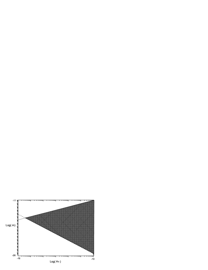
Figure 1: This plot shows the dependence of the curvaton mass, $m$, as a function of the Hubble parameter, $H_{*}$, according to Eqs. (18), (19) (dashed line), $m\leqslant 0.1H_{*}$ (solid line) and the inequality (23). The shadow zone shows the allowed values of $m$ and $H_{*}$ parameters.

In Fig. 1 we show the dependence of the curvaton mass, $m$ as a function of the Hubble parameter, $H_{*}$, according to Eqs.(18), (19), (23) and $m\leqslant 0.1H_{*}$. We have taken $P_{\zeta}=2.4\times 10^{-9}$.

Following the analysis done in Ref.A2 , we can obtain the behavior of the parameters $\gamma$ and $\alpha$ in all regions of the parameter space. This behavior is given in terms of the parameters $\lambda$, $A$ and $m$. In this aspect, we can determine the parameters in which the logamediate inflation together with the curvaton scenarios work. It is known that when $0\leq\gamma\leq 1$, inflation is generic for late times, and for any value of $\alpha$, and, in our case, it reads as follow, $\lambda\geq 1$ and $\alpha\geq 0$. For the case, when $\gamma>1$ and $\alpha\neq 0$, the models are noninflationary, because $\lambda<1$. When $\gamma<0$, $\alpha\geq 0$ or $\alpha<0$, this model does not work since $\lambda<-1$. For $\gamma>1$, $\alpha\neq 0$, or $\alpha=0$, these models never can inflate, due to $\lambda<1$ . In particular, if $\gamma=0$ (or equivalently $\lambda\rightarrow\infty$), this model does not work since from Eq. (22) $\Gamma_{\sigma}<0$. The case when $\alpha=0$ de Sitter solution is obtained and $\gamma=1$ ($\lambda=1$), and from Eq.(25) and the analysis done in Ref. R12 , we obtain the following constraint $1<A<10^{-4}/m^{2}$ in order to have a working model. For the cases $\gamma>1$ ($\lambda>1$) and $\alpha>0$, from Eq. (25) we find that our model works for $m^{2}<10^{-5}$ and $A>0$.

V Curvaton Decay Before Domination

On the other hand, considering that the curvaton $\sigma$ decays before it dominates the expansion (which we called the second scenario) and additionally, the mass of the curvaton is non-negligible when compared with the Hubble expansion rate $H$, i.e., $m\sim H$ and if the curvaton field decays at a time when $\Gamma_{\sigma}=H(a_{d})=H_{d}$, where ”d” stands for quantities at the time when the curvaton decays, we get that

$$\Gamma_{\sigma}=\;H_{d}=\;H_{k}\;\left(\frac{a_{k}}{a_{d}}\right)^{3},$$ (26)

where Eq.(11) is used.

If we allow the decaying of the curvaton after its mass becomes important, i.e. $\Gamma_{\sigma}<m$, and before that the curvaton dominates the cosmological expansion (i.e., $\Gamma_{\sigma}>H_{eq}$), we may write the constraint

$$\frac{\sigma_{*}^{2}}{6}<\frac{\Gamma_{\sigma}}{m}<1,$$ (27)

which is similar to that described in Ref.R21 .

In this scenario, the curvaton decays at the time when $\rho_{\sigma}<\rho_{\phi}$. Denoting the parameter $r_{d}$ as the ratio between the curvaton and the inflaton energy densities, evaluated at the time in which the curvaton decay occurs, i.e. at $a=a_{d}$, the parameter $P_{\zeta}$, becomes given by ref1u ; L1L2

$$P_{\zeta}\simeq\frac{r_{d}^{2}}{16\pi^{2}}\frac{H_{*}^{2}}{\sigma_{*}^{2}}.$$ (28)

Since $r_{d}=\left.\frac{\rho_{\sigma}}{\rho_{\phi}}\right|_{a=a_{d}}$, we get that $r_{d}=\frac{m^{2}\;\sigma_{*}^{2}\;a_{m}^{3}\;a_{d}^{3}}{6\;H_{k}^{2}\;a_{k}^{6}}$, where we have used $\rho_{\sigma}(a)=\frac{m^{2}\sigma_{*}^{2}}{2}\left(\frac{a_{k}}{a}\right)^{3}$ and $\rho_{\phi}(a)=\rho_{\phi}^{k}\left(\frac{a_{k}}{a}\right)^{6}$. Using Eqs.(12) and (26) we obtain

$$r_{d}=\;\frac{m\;\sigma_{*}^{2}}{6\;\Gamma_{\sigma}}.$$ (29)

The parameter $r_{d}$ is related to two other observable, the amount of non-Gaussianity, that is conventionally specified by a number $f_{NL}$ (NL meaning ”nonlinear”) S3 and the parameter of the isocurvature amplitude (or the ratio the isocurvature and adiabatic amplitudes at the pivot scale) S4 . Following, Ref.L1L2 the parameter $f_{NL}$, becomes of the order of $f_{NL}\simeq\frac{5}{4\,r_{d}}$, where this expression is only valid for high value of $f_{NL}$, which dominates over the intrinsic non-Gaussianity ( see Ref.S5 for the second order perturbations). From the observational data $f_{NL}<100$, therefore the parameter $r_{d}$ satisfies $r_{d}>0.01$M2 ; L1L2 .

From Eqs. (28) and (29) we find that $\sigma_{*}^{2}=576\;\pi^{2}\;\frac{P_{\zeta}}{m^{2}}\frac{\Gamma_{\sigma}^{2}}{H_{*}^{2}}\,$ and using that

$$H^{2}_{*}=H_{0}^{2}\,\left[B\,N_{*}+\,(\beta^{2}\gamma^{2}/2)^{\lambda/(\lambda-1)}\right]^{\frac{2(\lambda-1)}{\lambda}}\,\exp\left[-\beta\left(B\,N_{*}+(\beta^{2}\gamma^{2}/2)^{\lambda/(\lambda-1)}\right)^{1/\lambda}\right],$$ (30)

we get

$$\sigma_{*}^{2}=576\pi^{2}\frac{P_{\zeta}\;\Gamma_{\sigma}^{2}}{m^{2}\,H_{0}^{2}}\left[B\,N_{*}+\,(\beta^{2}\gamma^{2}/2)^{\lambda/(\lambda-1)}\right]^{\frac{2(1-\lambda)}{\lambda}}\,\exp\left[\beta\left(B\,N_{*}+(\beta^{2}\gamma^{2}/2)^{\lambda/(\lambda-1)}\right)^{1/\lambda}\right].$$ (31)

Thus, expressions (27) and (31) becomes useful for obtaining the following inequality for the decay parameter $\Gamma_{\sigma}$

$$\Gamma_{\sigma}<\frac{m\,H_{0}^{2}}{576\pi\,P_{\zeta}}\,\,\left[B\,N_{*}+\,(\beta^{2}\gamma^{2}/2)^{\lambda/(\lambda-1)}\right]^{\frac{2(\lambda-1)}{\lambda}}\,\exp\left[-\beta\left(B\,N_{*}+(\beta^{2}\gamma^{2}/2)^{\lambda/(\lambda-1)}\right)^{1/\lambda}\right].$$ (32)

We also derive a new constraint for the parameters $A$ and $\lambda$ characteristic of the logamediate inflationary universe model, by using the BBN temperature $T_{BBN}$. Since, the reheating temperature satisfies the bound $T_{reh}>T_{BBN}$, with $\Gamma_{\sigma}\,>\,T^{2}_{BBN}$ we get

$$H_{0}^{2}\,\left[B\,N_{*}+\,(\beta^{2}\gamma^{2}/2)^{\lambda/(\lambda-1)}\right]^{\frac{2(\lambda-1)}{\lambda}}\,\exp\left[-\beta\left(B\,N_{*}+(\beta^{2}\gamma^{2}/2)^{\lambda/(\lambda-1)}\right)^{1/\lambda}\right]$$

$$>\left(960\,\pi^{2}\right)^{2/3}\,P_{\zeta}^{2/3}\,T_{BBN}^{4/3}\sim 10^{-33}.$$ (33)

Here, we have used that $m\simeq H_{*}/10$ see Ref.dimo and Eqs. (27), (29) and (30).

From the hypothesis that $P_{\zeta_{\phi}}\lesssim\,0.0001\,P_{\zeta}$, we can set a new constraint for the decay parameter $\Gamma_{\sigma}$ given by

$$\Gamma_{\sigma}\lesssim\frac{10^{-2}}{12}\,\beta\,\gamma\,m\,\sigma_{*}^{2}\,\phi_{*}^{(1-\gamma)},$$

or equivalently,

$$\Gamma_{\sigma}\lesssim\,8\times 10^{-4}\,\beta\,\gamma\left[\frac{N_{*}}{A}\,\left(\frac{2(A\lambda)^{1/2}}{\lambda+1}\right)^{(\lambda+1)/2\lambda}+\left(\frac{\beta\gamma}{\sqrt{2}}\right)^{(\lambda-1)/\lambda}\right]^{(\lambda-1)/2\lambda}\,\;\;m\,\sigma_{*}^{2}.$$ (34)

Here, we have used Eqs. (20), (28) and (29).

On the other hand, if the decay rate is of gravitational strength, then $\Gamma_{\sigma}\sim m^{3}$ and the Eq.(32) is given by

$$m^{2}<\frac{\,H_{0}^{2}}{576\pi\,P_{\zeta}}\,\,\left[B\,N_{*}+\,(\beta^{2}\gamma^{2}/2)^{\lambda/(\lambda-1)}\right]^{\frac{2(\lambda-1)}{\lambda}}\,\exp\left[-\beta\left(B\,N_{*}+(\beta^{2}\gamma^{2}/2)^{\lambda/(\lambda-1)}\right)^{1/\lambda}\right],$$ (35)

and also the curvaton mass should obey the constraint $m^{2}\lesssim\frac{10^{-2}}{12}\,\beta\,\gamma\,\,\sigma_{*}^{2}\,\phi_{*}^{(1-\gamma)}$, where it was consider that $P_{\zeta_{\phi}}\lesssim\,0.0001\,P_{\zeta}$ as before.

VI Gravitational waves

Another set of bounds is due to the possible overproduction of the gravitational waves due to inflation. The corresponding gravitational wave amplitude can be written as

$$h_{GW}\simeq\,C_{1}\,H_{*},$$ (36)

where the constant $C_{1}\approx 10^{-5}$ Staro2 .

We may write the gravitational wave amplitude as function of the numbers of e-folds of inflation, i.e.

$$h_{GW}^{2}\simeq\,\;C_{1}^{2}\;\left[\frac{N_{*}}{A}+B\left(\frac{2}{\beta^{2}\gamma^{2}}\right)^{\frac{\gamma}{\gamma(2\gamma-1)}}\right]^{\frac{2(\lambda-1)}{\lambda}}\,\exp\left\{-\frac{2}{\gamma}\left[\frac{N_{*}}{A}+B\left(\frac{2}{\beta^{2}\gamma^{2}}\right)^{\frac{\gamma}{\gamma(2\gamma-1)}}\right]\right\},$$ (37)

where we have used Eq.(30).

After inflation the inflaton field follows an equation of state which is almost stiff and the spectrum of relic gravitons presents a characteristic in which the slope grows with the frequency (spike) for models that reenter the horizon during this epoch. This means that at high frequencies the spectrum forms a spike instead of being flat, as in the case of radiation dominated universeGi . Therefore, high frequency gravitons reentering the horizon during the kinetic epoch may disrupt BBN by increasing the Hubble parameter. This problem can be avoided if the following constraint on the density fraction of the gravitational wave is required R19 (see also Ref.dimo )

$$I\equiv\,h^{2}\,\int_{k_{BBN}}^{k_{*}}\;\Omega_{GW}(k)\,d\ln\,k\simeq\,2\,h^{2}\,\epsilon\,\Omega_{\gamma}(k_{0})\,h_{GW}^{2}\left(\frac{H_{*}}{\widetilde{H}}\right)^{2/3}\leq\,2\times 10^{-6},$$ (38)

where $\Omega_{GW}(k)$ is the density fraction of the gravitational wave with physical momentum $k$, $k_{BBN}$ is the physical momentum corresponding to the horizon at BBN, $\Omega_{\gamma}(k_{0})=2.6\times 10^{-5}h^{-2}$ is the density fraction of the radiation at present on horizon scales. Here, $h=0.73$ is the Hubble constant in which $H_{0}$ is in units of 100 km/sec/Mpc and $\epsilon\sim 10^{-2}$. The parameter $\widetilde{H}$ represents either $\widetilde{H}=H_{eq}$, when the curvaton decays after domination, or $\widetilde{H}=H_{d}$, if the curvaton decays before domination.

For the first scenario, the constraint on the density fraction of the gravitational wave, expressed by Eq.(38), becomes

$$\frac{m}{\sigma_{*}^{2}}\gtrsim\,\left(\frac{\,P_{\zeta}}{4\times 10^{5}}\right)^{2}\sim 10^{-28},$$ (39)

where we have used expressions (17), (36) and $C_{1}\sim 10^{-5}$. From Eqs.(18) and (39) we obtained that $m>10^{-34}$ and $10^{-40}/m<\sigma_{*}^{2}\lesssim 10^{28}\,m$.

For the second scenario, the constraint on the density fraction of the gravitational wave given by Eq.(38), becomes

$$\frac{m^{2}\;\sigma_{*}^{2}}{\Gamma_{\sigma}^{1/4}}\gtrsim\,6\times 10^{-5}\,P_{\zeta}\sim 10^{-13},$$ (40)

where we have used Eqs.(26) and (28). From Eqs.(27) and (40), we may write the inequality for the parameter given by $\Gamma_{\sigma}>10^{-19}\,m^{-4/3}$.

VII Conclusions

We have studied in detail the curvaton mechanism into the NO inflationary logamediate model. The curvaton scenario is responsible for reheating the Universe as well as for the curvature perturbations.

In describing the curvaton reheating we have considered two possible scenarios. In the first one, the curvaton dominates the universe after it decays and thus we have obtained the upper limit for $\Gamma_{\sigma}$ expressed by Eq.(21). In the second scenario the curvaton decays before domination. Here, we have also found a constraint for the values of $\Gamma_{\sigma}$ which is represented by Eq.(32).

During the scenario in which the curvaton decays after its dominates, our computations allow us to get the reheating temperature $T_{rh}\propto\Gamma_{\sigma}^{1/2}$ as hight as $10^{-12}$ (in units of $m_{p}$). Here, we have used Eq. (21), with $m\sim 10^{-8}$, $N_{*}=60$, $P_{\zeta}=2.4\times 10^{-9}$, $\lambda=5$ and $A\simeq 10^{-6}$ (see Ref.R12 for the values of $\lambda$ and $A$). In particular, for $\lambda=10$ and $A\simeq 10^{-15}$ we get that the reheating temperature is of the order of $10^{-16}$. In the case when $\lambda=2$ and $A\simeq 2\times 10^{-2}$ the reheating temperature is of the order of $T_{rh}\sim 10^{-21}$. If we consider the constraint from gravitational wave, we find that the inequalities for the scalar field $\sigma_{*}$ at the moment when the cosmological scales exit the horizon becomes $10^{-16}<\sigma_{*}<\sqrt{6}$.

In the second scenario, we could estimate the reheating temperature to be of the order of $\sim 10^{-13}$ as an upper limit from Eq.(27). Here, we have used $m\sim 10^{-8}$, $N_{*}=60$, $P_{\zeta}=10^{-10}$, $\lambda=5$ and $A\simeq 10^{-6}$. In particular, for $\lambda=10$ and $A\simeq 10^{-15}$ we estimate $T_{rh}\sim 10^{-17}$. For the values $\lambda=2$ and $A\simeq 2\times 10^{-2}$ the reheating temperature is of the order of $T_{rh}\sim 10^{-22}$. From the constraint of the gravitational wave we have obtained that $T_{rh}>10^{-13}$. Note that the value of this temperature does not agree with the previous value, this is due the fact that its value is obtained from different cosmological constraints. However, we have obtained values for the reheating temperature $T_{rh}$ which are in good agreement with those values reported previously in Refs.dimo ; cdch , which seriously challenges gravitino constraints, where the reheating temperature becomes of the order of $T_{rh}\sim 10^{-9}$ Elis .

- (1) A. Guth , Phys. Rev. D 23, 347 (1981); A.A. Starobinsky, Phys. Lett. B 91, 99 (1980); A.D. Linde, Phys. Lett. B 108, 389 (1982); idem Phys. Lett. B 129, 177 (1983); A. Albrecht and P. J. Steinhardt, Phys. Rev. Lett. 48,1220 (1982); K. Sato, Mon. Not. Roy. Astron. Soc. 195, 467 (1981).
- (2) V.F. Mukhanov and G.V. Chibisov , JETP Letters 33, 532(1981); S. W. Hawking, Phys. Lett. B 115, 295 (1982); A. Guth and S.-Y. Pi, Phys. Rev. Lett. 49, 1110 (1982); A. A. Starobinsky, Phys. Lett. B 117, 175 (1982); J.M. Bardeen, P.J. Steinhardt and M.S. Turner, Phys. Rev.D 28, 679 (1983).
- (3) G. Smoot, et al. Astrophys. J. Lett. 396, L1 (1992).
- (4) E. Komatsu et al. [WMAP Collaboration], Astrophys. J. Suppl. 180, 330 (2009).
- (5) L.P. Grishchuk, Sov. Phys. JETP 40, 409 (1975); A.A. Starobinsky, JETP Lett. 30, 682 (1979).
- (6) G. Efstathiou, C. Lawrence and J. Tauber (coordinators), ESASCI( 2005) 1.
- (7) http://lisa.jpl.nasa.gov/
- (8) D. H. Lyth and A. Riotto, Phys. Rept. 314, 1 (1999).
- (9) A. D. Linde (2005), hep-th/0503203.
- (10) J. D. Barrow, Class. Quant. Grav. 13, 2965 (1996).
- (11) J. D. Barrow and N. J. Nunes, Phys. Rev. D 76 043501 (2007).
- (12) P.G. Ferreira, M. Joyce, Phys.Rev.D 58, 023503 (1998).
- (13) P. Binetruy, Phys.Rev.D 60, 063502 (1999).
- (14) Ph. Brax, J. Martin, Phys.Lett.B 468, 40 (1999).
- (15) T. Damour, F. Piazza, G. Veneziano, Phys.Rev.D. 66, 046007 (2002).
- (16) Ph. Brax, J. Martin, Phys.Rev.D 61, 103502 (2000); S.C.C. Ng, N.J. Nunes, F. Rosati, Phys.Rev.D 64, 083510 (2001).
- (17) P.J.E. Peebles, B. Ratra, Rev.Mod.Phys.75, 559 (2003).
- (18) P. Parsons and J. D. Barrow, Phys. Rev. D 51, 6757 (1995).
- (19) E.W. Kolb and M.S. Turner, The Early Universe, Addison-Wesley, Menlo Park, CA, 1990.
- (20) L. Kofman and A. Linde, JHEP 0207, 004 (2002).
- (21) G. Felder, L. Kofman and A. Linde, Phys. Rev. D 60, 103505 (1999).
- (22) B. Feng and M. Li, Phys. Lett. B 564, 169 (2003).
- (23) M. Dine, L. Randall and S. Thomas, Nucl. Phys. B 458, 291 (1996); M. Dine, L. Randall and S. Thomas, Phys. Rev. Lett. 75, 398 (1995).
- (24) L.H. Ford, Phys. Rev. D 35, 2955 (1987).
- (25) A. R. Liddle and L. A. Ureña-López, Phys. Rev. D 68, 043517 (2003).
- (26) M. Sami, P. Chingangbam and T. Qureshi, Phys. Rev. D 66, 043530 (2002).
- (27) D. H. Lyth and D. Wands, Phys. Lett. B 524, 5 (2002).
- (28) T. Moroi and T. Takahashi , Phys. Lett. B 522, 215 (2001); K. Enqvist and M. Sloth , Nucl. Phys. B 626, 395 (2002); N. Bartolo and A. Liddle , Phys. Rev. D 65, 121301 (2002).
- (29) T. Moroi and H. Murayama, Phys. Lett. B 553, 126 (2003); K. Enqvist, S.Kasuya and A. Mazumdar, Phys. Rev. Lett. 90, 091302 (2003); M. Giovannini , Phys. Rev. D 67, 123512 (2003); M. Beltran, Phys. Rev. D 78, 023530 (2008); T. Moroi and T. Takahashi, Phys. Lett. B 671, 339 (2009).
- (30) S. Mollerach , Phys. Rev. D 42, 313 (1990).
- (31) K. Dimopoulos and D. H. Lyth, Phys. Rev. D 69, 123509 (2004).
- (32) M. Beltran, Phys. Rev. D 78, 023530 (2008).
- (33) A. R. Liddle and D. H. Lyth, ”Cosmological inflation and large-scale structure”, Cambridge University Press (2000).
- (34) K. Dimopoulos, D. H. Lyth and Y. Rodriguez, JHEP 0502, 055 (2005).
- (35) K. Dimopoulos, D. H. Lyth, A. Notari and A. Riotto, JHEP 0307, 053 (2003).
- (36) D. Langlois and F. Vernizzi, Phys. Rev. D 70, 063522 (2004).
- (37) J. D. Barrow, Phys. Rev. D 48, 1585 (1993).
- (38) M. Joyce and T. Prokopec, Phys. Rev. D 57, 6022 (1998).
- (39) Z. K. Guo, Y. S. Piao, R. G. Cai and Y. Z. Zhang, Phys. Rev. D 68, 043508 (2003).
- (40) J. C. Bueno Sanchez and K. Dimopoulos, JCAP 0711, 007 (2007).
- (41) M. Postma, Phys. Rev. D 67, 063518 (2003).
- (42) C. Campuzano, S. del Campo and R. Herrera, Phys. Lett. B 633, 149 (2006); idem, Phys. Rev. D 72, 083515 (2005); idem, JCAP 0606, 017 (2006).
- (43) E. Komatsu et al. [WMAP Collaboration], Astrophys. J. Suppl. 180, 330 (2009); J. Dunkley et al. [WMAP Collaboration], Astrophys. J. Suppl. 180, 306 (2009).
- (44) S. Mollerach, Phys. Rev. D 42, 313 (1990).
- (45) K. Dimopoulos, Phys. Lett. B 634, 331 (2006).
- (46) K. Dimopoulos, G. Lazarides, D. Lyth and R. Ruiz de Austri, Phys. Rev. D 68, 123515 (2003).
- (47) D. H. Lyth, C. Ungarelli and D. Wands, Phys. Rev. D 67, 023503 (2003).
- (48) E. Komatsu and D. N. Spergel, Phys. Rev. D 63, 063002 (2001).
- (49) R. Stompor, A. Banday and K. Gorski, Astrophys. J. Suppl. 170, 8 (1996).
- (50) N. Bartolo, S. Matarrese and A. Riotto, Phys. Rev. D 69, 043503 (2004).
- (51) A. Starobinsky , S. Tsujikawa and J. Yokoyama , Nucl.Phys.B 610, 383 (2001).
- (52) M. Giovannini, Phys. Rev. D 60, 123511 (1999); V. Sahni, M. Sami and T. Souradeep, Phys. Rev. D 65, 023518 (2002).
- (53) K. Dimopoulos, Phys. Rev. D 68, 123506 (2003).
- (54) J. R. Ellis, et al., Nucl. Phys. B 238, 453 (1984); M. Kawasaki and T. Moroi, Prog. Theor. Phys. 93, 879 (1995).