Adhesion of Multi-component Vesicle Membranes

Abstract

In this work, we study the adhesion of multi-component vesicle membrane to both flat and curved substrates, based on the conventional Helfrich bending energy for multi-component vesicles and adhesion potentials of different forms. A phase field formulation is used to describe the different components of the vesicle. For the axisymmetric case, a number of representative equilibrium vesicle shapes are computed and some energy diagrams are presented which reveal the dependence of the calculated shapes and solution branches on various parameters including both bending moduli and spontaneous curvatures as well as the adhesion potential constants. Our computation also confirms a recent experimental observation that the adhesion effect may promote phase separation in two-component vesicle membranes.

I Introduction

Adhesion is a fundamental step for many biological processes such as exocytosis, endocytosis. Cell adhesion also plays important roles in drug designs and drug deliveries as well as many biosensor applications Dunehoo ; lipowsky_book . There have been many experimental and theoretical studies focusing on this subject Das1 ; Gordon ; Lipowsky1 ; Lipowsky2 ; Fst07 . While many of the past studies on the vesicle-substrate adhesion have focused on the case of a flat substrate seifert1990 ; seifert1991 ; seifert1994 ; seifert1997 ; smith2003 ; cantat2003 ; ni2005 , there have also been some works that address the complexity of curved substrate. For instance, theoretical and experimental studies on the binding of a vesicle membrane to micro or nano-particles, or colloids have been conducted in dietrich1997 ; lipowsky1998 ; deserno2002 ; deserno2003 ; deserno2004 , where the characteristic spherical substrates have radii much smaller than that of the vesicles. In Das1 , the adhesion of a three dimensional vesicle to curved substrates has been studied where the curvature of the substrates are comparable to the curvature of the vesicles. A phase diagram for bound-unbound transitions has been presented. In this work, we study the adhesion of multi-component vesicle membranes to both flat and curved substrates. This is motivated by experimental studies of the modeled subjects. For instance in a recent experiment conducted by Gordon et al. Gordon , it was observed that a mixed-lipid membrane can go through a local phase separation above critical demixing temperature due to its close proximity to a biological or non-biological surface. That is, adhesion can promote the phase separation for the mixed-lipid cell or vesicle membranes.

In this work, we develop a phase field model to study the adhesion of multi-component vesicle membranes with a substrate through a specified adhesion potential. Following our recent approach described in JZhang , we take the adhesion potential to be a function of distance between the membrane and the substrate. The strength of adhesion potential is considered to be distinct for different components. By minimizing the total energy of the system that includes bending energy, interfacial line tension and the adhesion energy, the equilibrium vesicle shapes can be computed for a variety of parameter values. As the initial attempt, we consider the case that both the vesicle membrane and the substrate are axisymmetric to simplify the computation. We present, in particular, a number of typical equilibrium two-component axisymmetric vesicle profiles undergoing adhesion. The consistency between the phase field description and its sharp interface limit is also briefly discussed. Moreover, a numerical experiment is conducted to support the conclusion of Gordon that the adhesion may promote phase separation for a multi-component membrane.

II Multi-component vesicle membrane with adhesion

Equilibrium shapes of a multi-component vesicle are often described by minimizing an energy that includes elastic bending energy of the membrane and the line tension energy at the interface between the components Julicher . For the elastic bending energy of vesicle membrane, a common form adopted in the literature is that introduced by Helfrich Helfrich :

$$E_{b}=\int_{\Gamma}\Big{(}\lambda(H-a)^{2}+bK\Big{)}\ \text{d}\textbf{x}\,,$$ (1)

where $\Gamma$ is the membrane surface, $H$ and $K$ are the mean and Gaussian curvatures of $\Gamma$ with $\lambda$ and $b$ being the mean curvature bending modulus and the Gaussian curvature bending modulus respectively and $a$ is the spontaneous curvature. For simplicity, we consider the effect of mean curvature bending modulus and spontaneous curvature only. Thus $b$ is set to be zero and Eq. 1 becomes

$$E_{b}=\int_{\Gamma}\lambda(H-a)^{2}\text{d}\textbf{x}\,.$$

In this paper, we focus on two-component vesicle membranes which have the liquid-ordered and the liquid-disordered phases, and the two phases have distinct bending moduli and distinct spontaneous curvatures Baumgart1 ; Baumgart2 ; Das3 . Let $\Gamma_{1}$ and $\Gamma_{2}$ be the parts of the surface representing the two different phases with $\lambda_{1},\lambda_{2}$ being their corresponding bending moduli and $a_{1},a_{2}$ being their corresponding spontaneous curvatures, respectively. The total elastic bending energy for the two-component vesicle is

$$E_{b}=\int_{\Gamma_{1}}\lambda_{1}(H-a_{1})^{2}\ \text{d}\textbf{x}+\int_{\Gamma_{2}}\lambda_{2}(H-a_{2})^{2}\ \text{d}\textbf{x}\,.$$ (2)

The line tension energy, which is essentially an interfacial energy between the two phases is given as

$$E_{l}=\int_{\Gamma_{1}\cap\Gamma_{2}}\sigma\ \text{d}l\,,$$ (3)

where $\sigma$ is the constant line tension at the interface. Eqs (2) and (3) together define the total energy,

$$E=E_{b}+E_{l}\,,$$ (4)

with a minimum of $E$ describing the shape of an equilibrium two-component closed membrane.

Note that the vesicles or membranes discussed so far are free and not bounded to other objects. To incorporate the adhesive interaction with a substrate, an additional energetic contribution due to adhesion should be added to Eq. (4):

$$E_{\text{total}}=\int_{\Gamma_{1}}\lambda_{1}(H- a_{1})^{2}\ \text{d}\textbf{x}+\int_{\Gamma_{2}}\lambda_{2}(H-a_{2})^{2}\ \text{d}\textbf{x}$$

$$+\int_{\Gamma_{1}\cap\Gamma_{2}}\sigma\ \text{d}l-\int_{\Gamma}W(\textbf{x})\ \text{d}\textbf{x}\,,$$ (5)

where

$$W(\textbf{x})=\left\{\begin{array}[]{l}w_{1}\cdot P(\textbf{x}),\quad\textbf{x}\in\Gamma_{1}\\ w_{2}\cdot P(\textbf{x}),\quad\textbf{x}\in\Gamma_{2}\end{array}\right.$$ (6)

is the adhesion potential which varies with respect to the position x on $\Gamma=\Gamma_{1}\cup\Gamma_{2}$. In the above, $w_{1}$ and $w_{2}$ are the corresponding strengths of the adhesion potential experienced by the liquid-ordered and the liquid-disordered phases. A representative form of $W$ is that of a Gaussian form given by,

$$W(\textbf{x})=\left\{\begin{array}[]{l}w_{1}\exp(-\text{d}(\textbf{x})^{2}/\epsilon^{2}),\quad\textbf{x}\in\Gamma_{1}\\ w_{2}\exp(-\text{d}(\textbf{x})^{2}/\epsilon^{2}),\quad\textbf{x}\in\Gamma_{2}\end{array}\right.$$ (7)

where $\text{d}(\textbf{x})$ is the distance from x to a flat/curved substrate, and $\epsilon$ is a small number. Notice that when $\epsilon$ approaches zero, the adhesion potential converges to a sharp contact potential, a scenario that has been investigated in earlier studies Das1 ; Lipowsky2 . While we use the Gaussian potential (7) in most of this paper, to offer a comparison, we also consider the Leonard-Jones type potential,

$$W(\textbf{x})=\left\{\begin{array}[]{l}-w_{1}\cdot 4\bigg{[}\bigg{(}\dfrac{\beta}{\text{d}(\textbf{x})}\bigg{)}^{\alpha}-\bigg{(}\dfrac{\beta}{\text{d}(\textbf{x})}\bigg{)}^{\alpha/2}\bigg{]},\ \textbf{x}\in\Gamma_{1}\\ -w_{2}\cdot 4\bigg{[}\bigg{(}\dfrac{\beta}{\text{d}(\textbf{x})}\bigg{)}^{\alpha}-\bigg{(}\dfrac{\beta}{\text{d}(\textbf{x})}\bigg{)}^{\alpha/2}\bigg{]},\ \textbf{x}\in\Gamma_{2}\end{array}\right.$$ (8)

which induces a narrow repulsive region between vesicles and the substrate. The constant $\beta$ and the exponent $\alpha$ determine the thickness of the repulsive region and the rate of change of the adhesion potential, respectively.

II.1 Phase field formulation

To be able to effectively describe the different phases of the two-component vesicle, we use a phase field formulation which has become very popular in recent years in the modeling and simulations of vesicle deformations DLW04 ; DLRW05 ; misbah ; campelo ; lowengrub ; gao2009 ; JZhang . A phase field function can be used to describe the vesicle with the phase field bending energy as formulated in DLW04 ; DLRW05 . Adhesion energy can be incorporated into the phase field formulation as shown in JZhang . For multi-component vesicles, order parameters can be used to describe both the vesicle and its two components XWang . On the other hand, for a vesicle with a fixed topology, one can also use a direct (explicit) surface representation for the vesicle along with an order parameter (phase field function) to describe the two different phases of the membranelowengrub ; lowengrub02 . For the axisymmetric case considered here, it is particularly effective to adopt a sharp interface representation of the vesicle surface given by the revolution of a simple one-dimensional curve with an arc-length parametrization and a phase field representation of the different phases on the vesicle which is also a function of the arc-length.

Specifically, let $\Gamma$ be the vesicle surface, a phase field function $\eta=\eta(\textbf{x})$ is introduced over $\Gamma$ which may be used to represent either a material composition profile or a fictitious density of the lipids on the surface of the membrane and distinguishes between the liquid-ordered and liquid-disordered phases. As an illustration, we focus on the latter case so that in the liquid-ordered phase, $\eta$ is specified to be $+1$ and is colored as blue in figure 1; in the liquid-disordered phase, $\eta$ is assigned to be $-1$ and colored as red. In the interface between the liquid-ordered and liquid-disordered phases, $\eta$ rapidly, but continuously, changes from +1 to -1. Note that the phase field regularizes the sharp interface between the two different phases into a diffused one, and thus provides a more general depiction of the two-component vesicle in both the mixed and de-mixed states. The total energy (II) of the model in terms of the phase function $\eta$ is given by

$$E(\eta)=\int_{\Gamma}(c_{0}+c_{1}\eta) \big{[}H-a(c_{0}+c_{3}\eta)\big{]}^{2}\ \text{d}\textbf{x}$$

$$+\sigma\int_{\Gamma} \bigg{[}\dfrac{\xi}{2}\big{|}\nabla_{\Gamma}\eta\big{|}^{2}+\Phi(\eta)\bigg{]}\ \text{d}\textbf{x}$$

$$- \int_{\Gamma}w(c_{0}+c_{2}\eta)P(\text{d}(\textbf{x}))\ \text{d}\textbf{x}\,,$$ (9)

where the first and third terms are phase field formulas for elastic bending energy and adhesion energy, respectively. The term $c_{0}+c_{1}\eta$ is a phase field representation of $\lambda_{1}$ and $\lambda_{2}$. When x is away from the interfacial region, $c_{0}+c_{1}=\lambda_{1}$ and $c_{0}-c_{1}=\lambda_{2}$. The liquid-ordered phase is stiffer than the liquid-disordered phase, hence we always assume $c_{1}>0$. The term $a(c_{0}+c_{3}\eta)$ is considered as the phase field analog of spontaneous curvature, and

$$a(c_{0}+c_{3})=a_{1},\quad a(c_{0}-c_{3})=a_{2}$$

if x is away from the interfacial region. Similarly, $w(c_{0}+c_{2}\eta)P(\text{d}(\textbf{x}))$ is viewed as an approximation of the adhesion potential $W(\textbf{x})$, with

$$w(c_{0}+c_{2})=w_{1},\quad w(c_{0}-c_{2})=w_{2}$$

when x is far away from the interfacial region. The second term is a phase field approximation for the line tension energy where a double well potential function

$$\Phi(\eta)=\dfrac{1}{4\xi}(\eta^{2}-1)^{2}$$ (10)

is incorporated. $\nabla_{\Gamma}\eta$ is the surface gradient of $\eta$ which is the projection of $\nabla\eta$ onto the tangent plane of $\Gamma$. Notice that to make $\nabla_{\Gamma}\eta$ well defined, the function $\eta$ should be defined away from the membrane such that $\text{d}\eta/\text{d}\textbf{n}=0$ where n is the normal vector of $\Gamma$. The enclosed volume and total area of the membrane are assumed to be invariant. Meanwhile, the total amount of lipids is conserved. Thus three constraints are imposed during the minimization of the total energy (II.1):

$$\int_{\Gamma}\ \text{d}\textbf{x}=\text{A},\quad\int_{\Gamma}\ \text{d}V=\text{Vol},\quad\int_{\Gamma}\eta(\textbf{x})\ \text{d}\textbf{x}=C.$$ (11)

The constraint $\int_{\Gamma}\eta(\textbf{x})\ \text{d}\textbf{x}=C$ denotes the difference in the surface areas of the two phases in the sharp interface limit.

II.2 Axisymmetric Setting

In the present work, we focus on the axisymmetric membrane adhered on a flat/curved substrate. In this setting, the membrane surface is determined by evolving a 2-d curve. A vesicle with a flat substrate is schematically shown in figure 1. The axisymmetric vesicle surface is generated by evolving a curve parameterized by the arc-length $s$, and the total length of the generating curve is denoted by $\hat{s}$.

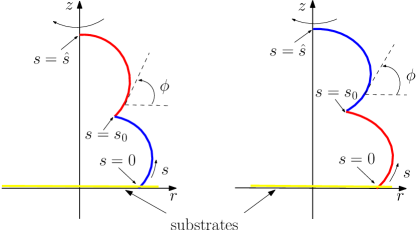
Figure 1: Schematic diagrams of axisymmetric two-component adhered vesicle membranes. Blue and red colors indicate the liquid-ordered and the liquid-disordered phases, respectively. $s=s_{0}$ specifies the phase boundary. Away from the interface, the blue phase has mean curvature bending modulus $c_{0}+c_{1}$ and adhesion potential $w(c_{0}+c_{2})P(\text{d}(\textbf{x}))$, while the red phase has mean curvature bending modulus $c_{0}-c_{1}$ and adhesion potential $w(c_{0}-c_{2})P(\text{d}(\textbf{x}))$.

The flat substrate is located at $z=0$ with the two different phases being distinguished by the red and blue colors. The transition point from red to blue is located at $s=s_{0}$. The figures on the left and right show different configurations with the blue phase and the red phase being adjacent to the substrate, respectively. For easy reference, we denote the left as red-blue vesicle membrane, and the right as blue-red vesicle membrane. The tangent angle $\phi$ is measured from the radial direction and $r$ is the distance of a point on the membrane from the axis of symmetry.

The mean curvature of the vesicle can be explicitly expressed by $r$ and $\phi$ as

$$H=\dfrac{1}{2}\Big{(}\phi^{\prime}+\dfrac{\sin\phi}{r}\Big{)},$$

where prime represents the derivative with respect to arc-length $s$. The line tension energy term in (II.1) becomes

$$2\pi\sigma\int_{0}^{\hat{s}}\dfrac{\xi}{2}\eta^{\prime 2}+\dfrac{1}{4\xi}(\eta^{2}-1)^{2}\ \text{d}s.$$

We nondimensionalize all the parameters and choose $c_{0}$ to be 1. Then the phase field model (II.1) is reduced to

$$E(\eta)=2\pi\int_{0}^{\hat{s}} (1+c_{1}\eta)\big{[}H-a(1+c_{3}\eta)\big{]}^{2}r\ \text{d}s$$

$$+2\pi\sigma \int_{0}^{\hat{s}}\bigg{[}\dfrac{\xi}{2}\eta^{\prime 2}+\dfrac{1}{4\xi}(\eta^{2}-1)^{2}\bigg{]}r\ \text{d}s$$

$$-2\pi\int_{0}^{\hat{s}}w(1+c_{2}\eta)P(\text{d}(\textbf{x}))\ r\ \text{d}s\,.$$ (12)

Additionally, the constraints (11) in the axisymmetric case lead to

$$(\cos T)^{\prime}=-r,$$ (13)

with $T$ being the arc-length parameter of the reference unit sphere,

$$\pi\int_{0}^{\hat{s}}r^{2}z^{\prime}ds=\text{Vol},$$ (14)

and

$$\int_{0}^{\hat{s}}\eta(s)rds=\text{C}\,.$$ (15)

The pointwise constraint (13), which is in fact equivalent to the one in (11), is referred as the lateral incompressibility condition for the membrane Das2 .

The shape of the membrane is determined by minimizing the total energy (II.2), subject to constraints (13), (14) and (15). It satisfies the Euler-Lagrange equations given by:

$$\big{[}\widetilde{H}^{\prime\prime}+\dfrac{r^{\prime}\widetilde{H}^{\prime}}{r}+2\widetilde{H} (H^{2}-K)+2a\widetilde{H}H(1+c_{3}\eta)\big{]}-2(\mu H+p+\tau\eta H)$$

$$+\sigma\xi\eta^{\prime 2}\phi^{\prime}-2\sigma H\Big{[}\dfrac{\xi}{2}\eta^{\prime 2}+\Phi(\eta)\Big{]}-w(1+c_{2}\eta)\bigg{(}\dfrac{dP}{d(\text{d}(\textbf{x}))}\dfrac{\delta(\text{d}(\textbf{x}))}{\delta\textbf{n}}-2HP\bigg{)}=0$$ (16)

$$c_{1}\big{[}H-a(1+c_{3}\eta)\big{]}^{2}-2ac_{3}\widetilde{H}+\sigma\Big{[}-\xi\Big{(}\eta^{\prime\prime}+\dfrac{r^{\prime}\eta^{\prime}}{r}\Big{)}+\dfrac{d\Phi}{d\eta}\Big{]}+\tau-c_{2}wP=0\,,$$ (17)

where $\widetilde{H}=(1+c_{1}\eta)\big{[}H-a(1+c_{3}\eta)\big{]}$ and $\mu,p$ and $\tau$ are the three Lagrange multipliers for the three constraints, respectively. The other equations from geometry are Das3 ; Jenkins :

$$\phi^{\prime}=2H-\dfrac{\sin\phi}{r},\quad r^{\prime}=\cos\phi,\quad z^{\prime}=\sin\phi.$$ (18)

Boundary conditions are imposed as follows:

$$H^{\prime}(0)=H^{\prime}(\hat{s})=0;\ r(0)=r(\hat{s})=0;$$

$$\phi(0)=0,\phi(\hat{s})=\pi;\ \eta^{\prime}(0)=\eta^{\prime}(\hat{s})=0.$$ (19)

III Numerical experiments

We numerically solve Eqs (II.2) through (18) subject to boundary condition (II.2) using the MATLAB ODE solver BVP4C. We tested the convergence of the computed results in our numerical simulation.

III.1 Adhesion with Gaussian potential

We first present the numerical results of a few adhered vesicles using the Gaussian adhesion potential.

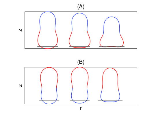
Figure 2: Membrane shapes for different $w$. Area=$4\pi$, volume=3.5, area difference $C=-0.3$, $\sigma=2$, $c_{1}=0.4$, $c_{3}=0$, $a=0$, $\xi=0.01$, $\epsilon=0.15$; (A) $c_{2}=-0.05$, $w=1.0,1.5,2.0$, from left to right; (B) $c_{2}=0.2$, $w=2.0,3.0,5.0$, from left to right.

In Figure 2, several numerical solutions for Eqs. (II.2) through (II.2) are shown. The curves are the cross-sections of the vesicle shapes with the blue-colored region representing the liquid-ordered phase and the red-colored region representing the liquid-disordered phase. The corresponding parameter values used in the experiments are taken as area=$4\pi$, volume=3.5, $C=-0.3$, $\sigma=2$, $c_{1}=0.4$, $c_{3}=0$, $a=0$, $\xi=0.01$, and $\epsilon=0.15$. Note that $c_{1}=0.4$ implies that the ratio $\lambda_{1}/\lambda_{2}=\lambda_{\text{blue}}/\lambda_{\text{red}}$ of the mean curvature bending moduli between the blue and red phases is 1.4/0.6. Moreover, $a=0$ and $c_{3}=0$ imply that both phases have zero spontaneous curvature. Blue-red adhered vesicles on flat substrate are shown in figure 2-A where $c_{2}=-0.05$, that is, $w_{1}/w_{2}=w_{\text{blue}}/w_{\text{red}}$ in (7) is equal to 0.95/1.05. Except the adhesion-associated parameter $w$, all the parameters are kept fixed as specified. Some adhered shapes of red-blue vesicles are shown in figure 2-B for various $w$ and $c_{2}=0.6$. Notice that there is a slight protrusion of vesicles into the flat substrate. This is due to the lack of repulsive effect in the Gaussian form of the adhesion potential.

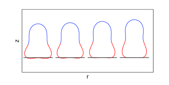
Figure 3: Convergence of adhered membranes as $\epsilon\rightarrow 0$. $\epsilon=0.15,0.10,0.05,0.01$, from left to right. Area=$4\pi$, volume=3.5, area difference $C=-0.3$, $\sigma=2$, $c_{1}=0.4$, $c_{2}=-0.05$, $c_{3}=0$, $a=0$, $\xi=0.01$, $w=2$.

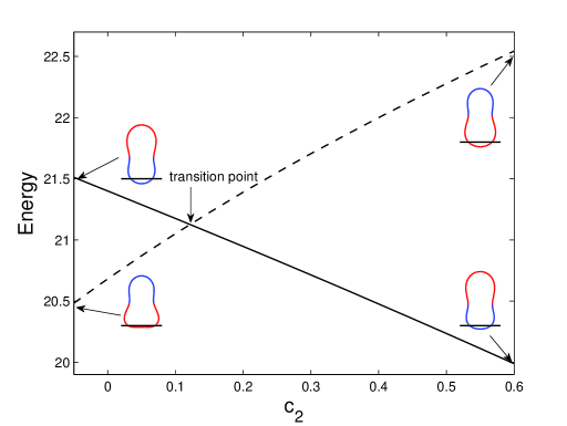
Figure 4: Energy comparison between blue-red vesicle and red-blue one. $w=2,c_{1}=0.3$ are fixed. $c_{2}$ varies from -0.05 to 0.6. The solid curve represents energy versus $c_{2}$ for the red-blue vesicle, while the dash curve is for the blue-red vesicle. The shapes of the vesicles at the four end-points of the curves are shown. Area=$4\pi$, volume=3.5, area difference $C=-0.3$, $\sigma=2$, $c_{3}=0$, $a=0$, $\xi=0.01$, $\epsilon=0.15$.

Convergence of the adhered vesicle shapes as $\epsilon$ approaches zero is presented in figure 3. Theoretically, by the standard asymptotic analysis, $\eta$ tends to converge to $\tanh\big{(}\frac{s-s_{0}}{\sqrt{2}\xi}\big{)}$ when $\xi$ approaches zero, where $s_{0}$ indicates the location of the interface which depends on the area difference $C$ (see appendix A). Numerically, for relatively larger $\epsilon$, the shapes of two-component vesicle membranes protrude into the flat substrate more significantly. As $\epsilon$ gets smaller, the protrusion becomes less visible and finally vanishes in the limit of $\epsilon\to 0$, that is the case corresponding to the effective contact potential Das1 ; JZhang ; Lipowsky2

$$W(\textbf{x})=\left\{\begin{array}[]{l}w\quad d(\textbf{x})=0\\ 0\quad\text{otherwise}.\end{array}\right.$$ (22)

Figure 4 shows the energy comparison between blue-red vesicle membrane and red-blue one under the influence of adhesion. Here area=$4\pi$, volume=3.5, $C=-0.3$, $\sigma=2$, $c_{1}=0.3$, $c_{3}=0$, $a=0$, $\xi=0.01$, $\epsilon=0.15$, $w=2.0$ are fixed. The two shapes on the left correspond to parameter $c_{2}=-0.05$ with $w_{\text{blue}}/w_{\text{red}}=0.95/1.05$. The blue-red vesicle, which is more deformed from the free vesicle shape, has lower energy and is more stable than the red-blue one in this case. On the other hand, the two shapes on the right correspond to $c_{2}=0.6$ leading to $w_{\text{blue}}/w_{\text{red}}=1.6/0.4$. There, the red-blue vesicle which is deformed more from the free shape has lower energy and is more stable than the blue-red one. In general, for $c_{2}<0$, $w_{\text{red}}$ is larger than $w_{\text{blue}}$ and blue-red membrane is more deformed from a free shape. Whereas, for $c_{2}>0$, $w_{\text{blue}}$ is larger than $w_{\text{red}}$ and red-blue membrane is more deformed from a free shape.

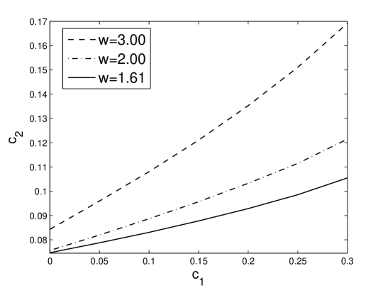
Figure 5: Transition curves for w=1.5, 2.0, 3.0. Above each curve, red-blue membrane is more stable; the blue-red membrane is more stable below the curves. The other parameter values are: Area=4$\pi$, volume=3.5, area difference $C=-0.3$, $\sigma=2$, $c_{3}=0$, $a=0$, $\xi=0.01$, $\epsilon=0.15$.

The energy comparison of the four shapes as discussed above may lead us to believe that the vesicle whose component adjacent to the substrate endures stronger adhesion is more stable. However, this is not always the case. As seen in figure 4, there is an anomalous region with $c_{2}$ between zero and 0.1217, and the blue phases suffer stronger adhesion but the blue-red vesicle is more stable. Outside this region, the shape with stronger adhesion on the component adjacent to the substrate is more stable. We observe that the existence of the region (0, 0.1217) is due to the nonzero values of $c_{1}$ and $C$ which model, in the two-component system, the effects due to the differences in the bending moduli and the surface areas of the two phases. When both $c_{1}$ and $C$ approach zero which is the limit where both components have the same bending moduli and equal surface areas, the multi-component vesicle reduces into a single component vesicle. And the anomalous region shrinks to the point $c_{2}=0$, also the transition point converges to $c_{2}=0$,

In addition, the transition point in figure 4 strongly depends on $c_{1}$ and the adhesion potential $w$. The dependence of the transition points on $c_{1}$ is shown in figure 5. For various $w=3.00,2.00,1.61$, we plot the transition curve $c_{1}$ versus $c_{2}$. The red-blue vesicle, corresponding to the parameter pair $(c_{1},c_{2})$ above each curve, is more stable; while the blue-red vesicle is more stable if the parameters $c_{1},c_{2}$ are chosen from the region below the transition curves.

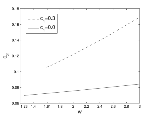
Figure 6: Dependence of $c_{2}$ on $w$ for phase transition when $c_{1}=0.3$ and 0.0, respectively. Area=4$\pi$, volume=3.5, area difference $C=-0.3$, $\sigma=2$, $c_{3}=0$, $a=0$, $\xi=0.01$, $\epsilon=0.15$.

Figure 5 shows that the transition always occurs for $c_{2}>0$. One may wonder if this is universally true for any adhesion potential $w$. The answer is provided via figure 6, the transition curve $w$ v.s. $c_{2}$ for fixed $c_{1}$. In figure 6, the dash curve corresponds to $c_{1}=0.3$, and the solid curve corresponds to $c_{1}=0$. Then we obtain the dependence of $c_{2}$ on $w$ when the transition occurs. For $c_{1}=0.3$, $w$ varies from 1.61 to 3; while for $c_{1}=0.0$, $w$ varies from 1.26 to 3. Above the transition curve, the red-blue vesicle is the more stable one; while below the curve, the blue-red vesicle is more stable. The bound blue-red vesicle with given parameters will break away from the adhered state around $w=1.60(1.25)$ when $c_{1}=0.3(0.0)$ and change to an unbound (free) vesicle. We can thus claim that $c_{2}$ is always positive for any bound adhesion potential $w$ when $c_{1}$ is fixed.

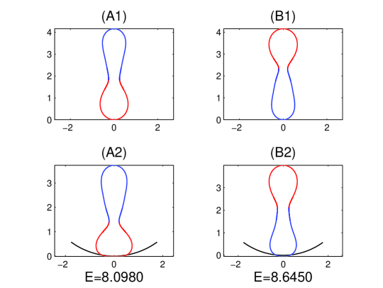
Figure 7: Effect of spontaneous curvatures on the vesicle shapes. Representative shapes of vesicle membranes are shown. Area=4$\pi$, volume=2.7, area difference $C=0$, $\sigma=1$, $c_{1}=0.0$, $c_{2}=0$ $c_{3}=0.5$, $a=2/3$, $\xi=0.01$, $\epsilon=0.05$, $w=2$.

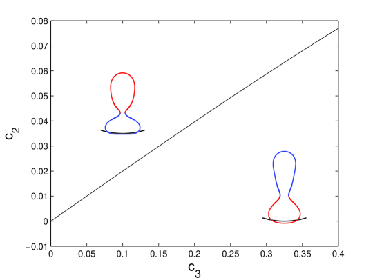
Figure 8: Dependence of $c_{2}$ on $c_{3}$ for phase transition. Representative shapes of vesicle membranes are shown above or below the transition curve. area=$4\pi$, volume=$2.7$, area difference $C=0$, $\sigma=1$, $c_{1}=0.0$, $a=2/3$, $\xi=0.01$, $\epsilon=0.15$, $w=2$.

We also take the effects of the spontaneous curvature and the substrate curvature into consideration Ursell ; Das4 . In figure 7 the flat substrate is now replaced by a concave-up spherical substrate with radius $R=3$. Here area=$4\pi$, volume=$2.7$, area difference $C=0$, $\sigma=1$, $c_{1}=0$, $c_{2}=0$, $c_{3}=0.5$, $a=2/3$, $\xi=0.01$ and $\epsilon=0.05$. We take $w=0$ and $w=2$ respectively to find both free vesicles and adhered vesicles. Differing from the previous figures in this subsection, the red and blue colors in this experiment indicate the phases having different spontaneous curvatures. The blue phase has a bigger spontaneous curvature $a(1+c_{3})=1$ while the red phase has a smaller one $a(1-c_{3})=1/3$. A1 and B1 show the free vesicles with specified parameters. Notice that the red phase, which possesses a smaller spontaneous curvature, has shapes less elongated than the blue phase. A2 and B2 are adhered blue-red and red-blue vesicles. By comparing the total energy of these two adhered vesicle, we find out that the blue-red vesicle with the red phase at bottom, whose spontaneous curvature matches with the curvature of the curved substrate, is more stable than the red-blue vesicle.

We choose here a volume with value 2.7 which is smaller than the previously chosen value of 3.5 because larger osmotic pressure difference makes the effect of spontaneous curvatures on the vesicle shapes more visible.

Similar to the discussion of stability transition in figure 5 and figure 6, when the spontaneous curvature effect is taken into account, we can also find the dependence of transition points on $c_{1},c_{2},c_{3},w$. Without repeatedly showing many figures, we present here only the transition curve $c_{3}$ v.s. $c_{2}$ in figure 8 with $c_{1}=0,w=2$ fixed. Other parameters are set as area=$4\pi$, volume=$2.7$, area difference $C=0$, $\sigma=1$, $a=2/3$, $\xi=0.01$, $\epsilon=0.15$. Above the transition curve, a representative red-blue vesicle is shown which is more stable than the blue-red vesicle; while below the transition curve, the blue-red vesicle is more stable.

III.2 Adhesion with Leonard-Jones potential

When the Gaussian adhesion potential is used, as seen in the above, slight protrusion of vesicles into the substrate may occur. If this protrusion is of any practical concern, one possible way to avoid the protrusion is to replace the Gaussian adhesion potential by a Leonard-Jones type potential. We demonstrate, by employing the following potential,

$$P(\text{d}(\textbf{x}))=-4\bigg{[}\bigg{(}\dfrac{\beta}{\text{d}(\textbf{x})}\bigg{)}^{\alpha}-\bigg{(}\dfrac{\beta}{\text{d}(\textbf{x})}\bigg{)}^{\alpha/2}\bigg{]}\,,$$ (23)

that the shapes of adhered vesicles without any protrusion can be obtained using our phase field formulation. The key difference between the Gaussian type potential (7) and the Leonard-Jones type potential (23) is that Gaussian potential is globally attractive, while there is a narrow region with $\text{d}(\textbf{x})$ between zero and $\beta$ where the Leonard-Jones type potential is repulsive. Such a repulsive region can prevent the vesicle membrane from protruding into the substrate.

An axisymmetric simulation is shown in figure 9 where we take $\alpha=5$. In figure 9(A), $w=2$ is fixed, and the parameter $\beta$ is decreased from left to right. We can see that the repulsive region between substrate and vesicle membrane narrows down. The shape deformation under the influence of adhesion is shown in figure 9(B) where the repulsive region is fixed but $w$ is increased from left to right. The stability transition curves, similar to that obtained previously for Gaussian potential, can also be obtained for Leonard-Jones type potential. Given the similarities in the findings, we do not repeat the discussion here.

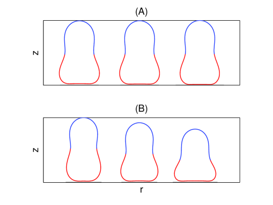
Figure 9: Membrane shapes for Leonard-Jones type potential. (A) $w=2$, $\beta=0.05,0.035,0.025$, from left to right; (B) $\beta=0.05$, $w=1.2,2.0,2.8$, from left to right. Other parameters: Area=$4\pi$, volume=3.5, area difference $C=-0.3$, $\sigma=2$, $c_{1}=0.3$, $c_{2}=-0.05$, $c_{3}=0$, $a=0$, $\xi=0.01$, $\alpha=5$

III.3 Promotion of phase separation

In this subsection, two numerical experiments are presented to support Gordon and coworkers’ experimental observation that adhesion may promote the phase separation Gordon . The experiments involve the phase field simulations for relatively large diffuse interface parameter $\xi$ which is consistent to the experimental setting. The Leonard-Jones type adhesion potential is employed in this subsection.

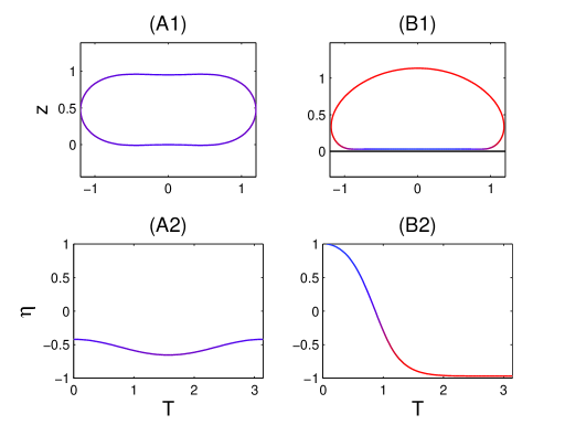
Figure 10: Adhesion induces phase separation. An almost homogeneous free vesicle is phase-separated by a Leonard-Jones adhesion.

In the first experiment, the function $\eta(s)$ is viewed as a chemical composition function, which can be considered as a compositional fluctuation around a homogeneous state with composition $\eta_{0}$. The constraint (15) is specified as

$$\int_{0}^{\hat{s}}\eta(s)rds=\int_{0}^{\hat{s}}\eta_{0}rds$$ (24)

We now demonstrate that for an equilibrium free vesicle with associated $\eta(s)$ almost homogeneous, namely $\eta(s)\approx\eta_{0}$, after adding the adhesion, it displays the phase separation behavior with $\eta(s)$ changing into a tanh-like profile representing two distinct phases.

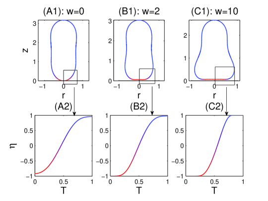
Figure 11: Promotion of phase separation. As $w$ gets bigger, the two phases of $\eta$ near the interfacial region are separated more. Area=4$\pi$, volume=3.5, area difference $C=1.7$, $\xi=0.13$, $\sigma=1$, $c_{1}=0.05$, $c_{2}=-1.00$, $c_{3}=0$, $\zeta=1$, $\beta=0.05$, $\alpha=5$.

The numerical experiment is presented in figure 10. In (A1-2), for $\text{area}=4\pi,\text{volume}=3.5,\eta_{0}=-1/\sqrt{3},\xi=0.33,\sigma=5/(1-0.8\eta_{0}),c_{1}=0.8/(1-0.8\eta_{0}),c_{2}=1.0/(1-1.0\eta_{0}),c_{3}=0$, a free vesicle is computed first. The chemical composition function $\eta$ and the associated vesicle profile shown in (A1-2) correspond to the stable energy minimum (in the absence of adhesion). The change in composition is relatively small, representing a state of mixed phases in much of the vesicle. By adding Leonard-Jones adhesion with $w=5(1-1.0\eta_{0})/(1-0.8\eta_{0}),\beta=0.023,\alpha=5$, an adhered vesicle with associated $\eta$ corresponding to the new energy minimizer is shown in (B1-2). A phase separation occurs with a much more significant phase difference $\max(\eta)-\min(\eta)=1.9703$ in (B2). In comparison, we have $\max(\eta)-\min(\eta)=0.2345$ in (A2), which is only $11.90\%$ of the phase difference for adhered vesicle. We thus see that adhesion can significantly promote phase separation. Furthermore, the bending modulus of the phase-mixed vesicle $\lambda_{\text{mixed}}$ is roughly around $1/(1-0.8\eta_{0})$, and the bending moduli of the phase-separated vesicle are $\lambda_{\text{blue}}=2.2649/(1-0.8\eta_{0})$ and $\lambda_{\text{red}}=0.6873/(1-0.8\eta_{0})$. These parameter values imply that $\lambda_{\text{red}}\approx\lambda_{\text{mixed}}$ and $\lambda_{\text{blue}}/\lambda_{\text{red}}=3.2954$ which agree with the ratios of the bending stiffnesses of the ordered, the disordered and the mixed phases available in the literature Gordon ; Roux ; Baumgart2 ; Baumgart1 .

The effect of adhesion on phase separation can be further demonstrated in the next experiment. Here again, we take the order parameter $\eta(s)$ to be a labeling function for relative lipid density which stays within $[-1,1]$. To model a wider diffuse interfacial layer corresponding to a relatively large $\xi$ and yet maintain the bound on $\eta$, we replace the double well potential function (10) by the following double obstacle potential function elliott :

$$(1+\eta)\ln(1+\eta)+(1-\eta)\ln(1-\eta)+\gamma(1-\eta^{2})-2\ln 2\;.$$ (25)

where $\gamma=1+2\ln 2$ is a constant describing the height of the potential barrier.

Figure 11 shows a numerical experiment while we choose $\xi=0.13$ so that for unbounded vesicles, there would be a wide interfacial regions with less dramatic phase separation effect. Then for various $w=0,2,10$, we compute the corresponding adhered vesicle shapes and the corresponding lipid density functions $\eta$. We highlight the densities near the interfacial region (the boxed portion of the vesicle profile). With the plots using the same scaling in the arc-length, one can see that with a larger adhesion strength $w$, the interfacial layer gets narrower and the separation between the red and blue phases becomes sharper and more dramatic.

IV Conclusion

In this work, we develop a phase field model for the adhesion of the multi-component vesicle membrane to a flat/curved substrate. Some representative vesicle shapes are presented. The influence of $c_{2}$, which measures the contrast of the adhesion effect for the different phases, on the stability of membrane shapes is discussed here. It turns out that the multi-component vesicle, whose lower part suffers stronger adhesion, is more stable in most cases. We also consider the the phase transition from blue-red vesicle to red-blue vesicle, and the influence of other parameters such as the relative contribution of the adhesion and the bending energy. The effect of spontaneous curvature is also numerically observed by examining the adhesion of the vesicles on a curved substrate. We also present vesicle shapes corresponding to the Leonard-Jones type adhesion potential to show that the repulsive region can effectively prevent the protrusion of the vesicles into the substrates should this be of practical concern. Finally, we numerically examine the fact that adhesion can promote the phase separation for multi-component vesicle membrane.

Although the numerical studies presented here are focusing on the axisymmetric configuration, the phase field formulation is applicable to more general settings such as in the study of the interaction between the multi-component vesicle and a patterned substrate. It can also be used to extend the study of membrane-mediated particle interactions deserno2003 ; deserno2004 to multi-component vesicles. The present phase field formulation of the multi-component vesicle and substrate interaction can also be extended in several directions. For instance, by incorporating the Gaussian curvature contributions to the bending energy, fusion of multi-component vesicles can be studied. By adding an entropic contribution to the free energy, we can also consider the weak adhesion regime where fluctuation of the vesicle shape due to thermal excitation plays an important role.

Appendix A Asymptotic analysis for $\eta$

In section III, the convergent behavior of the adhered vesicles as the interfacial width $\epsilon$ approaches zero is briefly mentioned. It is claimed that the phase field function $\eta$ approaches $\tanh\big{(}\frac{s-s_{0}}{\sqrt{2}\xi}\big{)}$ as the parameter $\xi$ approaches zero. A boundary layer calculation is carried out to support such an observationHolmes .

The lipid density function $\eta(s)$ is governed by the Eq (17) and can be rewritten as

$$\xi\Big{(}c_{1}\big{[}H-a(1 +c_{3}\eta)\big{]}^{2}-2ac_{3}\widetilde{H}+\tau-c_{2}wP\Big{)}r$$

$$+\sigma\Big{[}-\xi^{2}(\eta^{\prime}r)^{\prime}+(\eta^{2}-1)\eta r\Big{]}=0$$ (26)

An asymptotic analysis in the sharp interface limit is carried out as follows. For simplicity, we only consider the O(1) terms for outer and inner layers here. The inner layer and the outer layer are the regions around the interface and away from the interface, respectively.

Within the outer layer, $\eta$ does not change much with respect to the arc-length and we expand $\eta(s)$ as

$$\eta(s)\sim\eta_{0}(s)+\xi\eta_{1}(s)+\ldots\,,$$ (27)

We substitute (27) into (A) and obtain an equation for $\eta_{0}$ at the lowest order:

$$(\eta_{0}^{2}-1)\eta_{0}r=0\,.$$

The solutions are

$$\eta_{0}=0,\pm 1\,,$$

and we choose $\eta=1$ and $\eta=-1$ in the two sides of the interface to represent the blue and red phases, respectively. Here let us assume $\eta=-1$ in the side $s<s_{0}$; and $\eta=1$ in the side $s>s_{0}$.

In the inner layer, we expect $\eta$ to vary rapidly from $-1$ to $1$ and introduce a new stretched arc-length variable

$$S=\dfrac{s-s_{0}}{\xi^{\mu}}\,,$$

where $\mu$ is an yet undetermined parameter. We now express $\eta$ as a function of the stretched variable $S$ and expand $\eta$ as

$$\widetilde{\eta}(S)\sim\widetilde{\eta}_{0}(S)+\xi\widetilde{\eta}_{1}(S)+\cdots\,.$$ (28)

Notice that

$$r(s)=r(s_{0}+\xi^{\mu}S)=r(s_{0})+\xi^{\mu}Sr^{\prime}(s_{0})+O(\xi^{2\mu}),$$

Upon rewriting Eq. (A) in terms of the stretched variable $S$ and, subsequently, using Eq. (28) we obtain

$$- \xi^{2-2\mu}r(s_{0})\dfrac{d^{2}\widetilde{\eta}_{0}}{dS^{2}}-\xi^{2-\mu}r^{\prime}(s_{0})\dfrac{d}{dS}\Big{(}S\dfrac{d\widetilde{\eta}_{0}}{dS}\Big{)}$$

$$+(\widetilde{\eta}_{0}^{2}-1)\widetilde{\eta}_{0}\big{[}r(s_{0})+\xi^{\mu}Sr^{\prime}(s_{0})\big{]}+O(\xi^{\mu})=0$$ (29)

There are two possible choices for $\mu$. If $\mu$ balances the second and third terms, namely, $2-\mu=0$. Then the leading order term is:

$$-r(s_{0})\dfrac{d^{2}\widetilde{\eta}_{0}}{dS^{2}}=0$$

which implies $\widetilde{\eta}_{0}=aS+b$. However, this solution does not satisfy the matching conditions

$$\widetilde{\eta}_{0}(-\infty)=\eta_{0}(0)=-1,\quad\widetilde{\eta}_{0}(+\infty)=\eta_{0}(\hat{s})=1\,.$$

Another choice is to balance the first and third terms of equation (A), namely, $\mu=1$, and one gets the leading order term:

$$-r(s_{0})\dfrac{d^{2}\widetilde{\eta}_{0}}{dS^{2}}+(\widetilde{\eta}_{0}^{2}-1)\widetilde{\eta}_{0}r(s_{0})=0.$$

If the boundary condition $\widetilde{\eta}_{0}(-\infty)=-1,\widetilde{\eta}_{0}(+\infty)=+1$ are imposed, a typical solution of the above nonlinear equation, which satisfies the matching condition, is

$$\widetilde{\eta}_{0}(S)=\tanh\Big{(}\dfrac{S}{\sqrt{2}}\Big{)}.$$

Then the composite solution of (A), given by

inner solution + outer solution - matching solution,

takes the form

$$\widetilde{\eta}_{0}(S)+\eta_{0}^{-}(s)-\eta_{0}^{-}(0)+\eta_{0}^{\text{+}}(s)-\eta_{0}^{\text{+}}(\hat{s}),$$

and explicitly

$$\eta(s)\sim\tanh\Big{(}\dfrac{s-s_{0}}{\sqrt{2}\xi}\Big{)}+\ldots$$

References

- (1) A. L. Dunehoo, M. Anderson, S. Majumdar, N. Kobayashi, C. Berkland, and T. J. Siahaan, “Cell adhesion molecules for targeted drug delivery,” Journal of Pharmaceutical Sciences 95-9, 1856–1872 (2006)
- (2) Structure and Dynamics of Membranes, Handbook of Biological Physics Vol. 1, edited by R. Lipowsky and E. Sackmann (Elsevier, Amsterdam, 1995)
- (3) S. Das and Q. Du, “Adhesion of vesicles to curved substrates,” Physical Review E 77, 011907 (2008)
- (4) V. D. Gordon, M. Deserno, C. M. J. Andrew, S. U. Egelhaaf, and W. C. K. Poon, “Adhesion promotes phase separation in mixed-lipid membranes,” Europhysics Letters 84, 48003 (2008)
- (5) R. Lipowsky, M. Brinkmann, R. Dimova, C. Haluska, J. Kierfeld, and J. Shillcock, “Wetting, budding, and fusion - morphological transitions of soft surfaces,” Journal of Physics: Condensed Matter 17, S2885–S2902 (2005)
- (6) R. Lipowsky, “The conformation of membranes,” Nature 349, 475–481 (1991)
- (7) C. Funkhouser, F. Solis, and K. Thorton, “Coupled composition-deformation phase-field method for multicomponent lipid membranes,” Physical Review E 76, 011912 (2007)
- (8) U. Seifert and R. Lipowsky, “Adhesion of vesicles,” Physical Review A 42, 4768–4771 (1990)
- (9) U. Seifert, “Adhesion of vesicles in two dimensions,” Physical Review A 43, 6803–6814 (1991)
- (10) U. Seifert and S. A. Langer, “Hydrodynamics of membranes: the bilayer aspect and adhesion,” Biophysical Chemistry 49, 13–22 (1994)
- (11) U. Seifert, “Configurations of fluid membranes and vesicles,” Advances in Physics 46, 13–137 (1997)
- (12) A.-S. Smith, E. Sackmann, and U. Seifert, “Effects of a pulling force on the shape of a bound vesicle,” Europhysics Letters 64, 281–287 (2003)
- (13) I. Cantat, K. Kassner, and C. Misbah, “Vesicles in hepatotaxis with hydrodynamical dissipation,” The European Physical Journal E 10, 175–189 (2003)
- (14) D. Ni, H. Shi, and Y. Yin, “Theoretical analysis of adhering lipid vesicles with free edges,” Colloids and Surfaces B 46, 162–168 (2005)
- (15) C. Dietrich, M. Anglova, and B. Pouligny, “Adhesion of latex spheres to giant phospholipid vesicles: statics and dynamics,” Journal of Physics II 7, 1651–1682 (1997)
- (16) R. Lipowsky and H.-G. Döbereiner, “Vesicles in contact with nanoparticles and colloids,” Europhysics Letters 43, 219–225 (1998)
- (17) M. Deserno and W. M. Gelbart, “Adhesion and wrapping in colloid-vesicle complexes,” Journal of Physical Chemistry B 106, 5543–5552 (2002)
- (18) M. Deserno and T. Bickel, “Wrapping of a spherical colloid by a fluid membrane,” Europhysics Letters 62, 767–773 (2003)
- (19) M. Deserno, “Elastic deformation of a fluid membrane upon colloid binding,” Physical Review E 69, 031903 (2004)
- (20) J. Zhang, S. Das, and Q. Du, “A phase field model for vesicle substrate adhesion,” Journal of Computational Physics 228, 7837–7849 (2009)
- (21) F. Julicher and R. Lipowksy, “Shape transformations of vesicles with intramembrane domains,” Physical Review E 53-3, 2670 (1996)
- (22) W. helfrich, “Elastic properties of lipid bilayers theory and possilbe experiments,” Z. Naturforsch 28c, 693–703 (1973)
- (23) T. Baumgart, S. Das, W. W. Webb, and J. T. Jenkins, “Membrane elasticity in giant vescles with fluid phase coexistence,” Biophysiccal Journal 89, 1067–1080 (2005)
- (24) T. Baumgart, S. Hess, and W. W. Webb, “Imaging coexisting fluid domains in biomembrane models coupling curvature and line tension,” Nature 425, 821–824 (2003)
- (25) S. Das, Studies of axisymmetric lipid bilayer vesicles: parameter estimation, micropipette aspiration, and phase transition (Phd thesis, 2007)
- (26) Q. Du, C. Liu, and X. Wang, “A phase field approach in the numerical study of the elastic bending energy for vesicle membranes,” Journal of Computational Physics 198, 450–468 (2004)
- (27) Q. Du, C. Liu, R. Ryham, and X. Wang, “Modeling the spontaneous curvature effects in static cell membrane deformations by a phase field formulation,” Communication in Pure and Applied Analysis 4, 537–548 (2005)
- (28) K. Kassner T. Biben and C. Misbah, “Phase-field approach to three-dimensional vesicle dynamics,” Physical Review E 72, 041921 (2005)
- (29) F. Campelo and A. Hernandez-Machado, “Dynamic model and stationary shapes of fluid vesicles,” Eur. Phys. J. E 20, 37–45 (2006)
- (30) J. S. Sohn, Y. H. Tseng, S. Li, A. Voigt, and J. S. Lowengrub, “Dynamics of multicomponent vesicles in a viscous fluid,” Journal of Computational Physics 229, 119–144 (2010)
- (31) L. Gao, X. Feng, and H. Gao, “A phase field method for simulating morphological evolution of vesicles in electric fields,” Journal of Computational Physics 228, 4162–4181 (2009)
- (32) X. Wang and Q. Du, “Modeling and simulations of multi-component lipid membranes and open membranes via diffuse interface approaches,” Journal of Mathematical Biology 56, 347–371 (2008)
- (33) J. S. Lowengrub, A. Ratz, and A. Voigt, “Phase-field modeling of the dynamics of multicomponent vesicles: Spinodal decomposition, coarsening, budding, and fission,” Physical Review E 79, 031926 (2009)
- (34) S. Das and J. T. Jenkins, “A higher-order boundary layer analysis for lipid vesicles with two fluid domians,” J Fluid Mech 597, 429–448 (2008)
- (35) J. T. Jenkins, “Static equilibrium configurations of a model red blood cell,” Journal of Mathematical Biology 4, 149–169 (1977)
- (36) T. S. Ursell, W. S. Klug, and R. Philips, “Morphology and interaction between lipid domains,” PNAS 106, 13301–13306 (2009)
- (37) S. L. Das, J. T. Jenkins, and T. Baumgart, “Neck geometry and shape transitions in vesicles with co-existing fluid phases: Role of gaussian curvature stiffness versus spontaneous curvature,” Europhysics Letters 86, 48003 (2009)
- (38) A. Roux, D. Cuvelier, P. Nassoy, J. Prost, P. Bassereau, and B. Goudh, “Role of curvature and phase transition in lipid sorting and fission of membrane tubules,” EMBO Journal 24, 1537–1545 (2005)
- (39) J. Blowey and C. Elliott, “A phase field model with a doble obstacle potential,” Motion by mean curvature and related topics: proceedings of the international conference held at Trento, July 20-24, 1992, 1–22(1994)
- (40) M. H. Holmes, Introduction to perturbation methods, Texts in applied mathematics 20 (Springer-Verlag, 1995)