Asymptotic properties of U-processes under long-range dependence

Abstract

Let $(X_{i})_{i\geq 1}$ be a stationary mean-zero Gaussian process with covariances $\rho(k)=\mathbb{E}(X_{1}X_{k+1})$ satisfying: $\rho(0)=1$ and $\rho(k)=k^{-D}L(k)$ where $D$ is in $(0,1)$ and $L$ is slowly varying at infinity. Consider the $U$-process $\{U_{n}(r),\;r\in I\}$ defined as

$$U_{n}(r)=\frac{1}{n(n-1)}\sum_{1\leq i\neq j\leq n}\mathbbm{1}_{\{G(X_{i},X_{j})\leq r\}}\;,$$

where $I$ is an interval included in $\mathbb{R}$ and $G$ is a symmetric function. In this paper, we provide central and non-central limit theorems for $U_{n}$. They are used to derive, in the long-range dependence setting, new properties of many well-known estimators such as the Hodges-Lehmann estimator, which is a well-known robust location estimator, the Wilcoxon-signed rank statistic, the sample correlation integral and an associated robust scale estimator. These robust estimators are shown to have the same asymptotic distribution as the classical location and scale estimators. The limiting distributions are expressed through multiple Wiener-Itô integrals.

, , , and t1Corresponding author t2Murad S. Taqqu would like to thank Telecom ParisTech for their hospitality. This research was partially supported by the NSF Grants DMS-0706786 and DMS-1007616 at Boston University.

1 Introduction

Since the seminal work by Hoeffding (1948), $U$-statistics have been widely studied to investigate the asymptotic properties of many statistics such as the sample variance, the Gini’s mean difference and the Wilcoxon one-sample statistic, see Serfling (1980) for other examples. One of the most powerful tools used to derive the asymptotic behavior of $U$-statistics is the Hoeffding’s decomposition [Hoeffding (1948)]. In the i.i.d and weak dependent frameworks, it provides a decomposition of a $U$-statistic into several terms having different orders of magnitudes, and in general the one with the leading order determines the asymptotic behavior of the $U$-statistic, see Serfling (1980), Borovkova, Burton and Dehling (2001) and the references therein for further details. A recent review of the properties of $U$-statistics in various frameworks is presented in Hsing and Wu (2004). In the case of processes having a long-range dependent structure, decomposition ideas are also crucial. However, in the case of Gaussian long-memory processes, the classical Hoeffding’s decomposition may not provide the complete asymptotic behavior of $U$-statistics because all terms of this decomposition may contribute to the limit, see for example Dehling and Taqqu (1991). In this case, the asymptotic study of $U$-statistics can be achieved by using an expansion in Hermite polynomials, see Dehling and Taqqu (1989, 1991). For a large class of processes including linear and nonlinear processes, a new decomposition is discussed in Hsing and Wu (2004). These authors use martingale-based techniques to establish the asymptotic properties of $U$-statistics.

A very natural extension of $U$-statistics (which are random variables) is the notion of $U$-processes which encompasses a wide class of estimators. For example, Borovkova, Burton and Dehling (2001) study the Grassberger-Proccacia estimator which can be used to estimate the correlation dimension. In Section 5 of their work, the authors investigate the asymptotic properties of $U$-processes when the underlying observations are functionals of an absolutely regular process, that is, short-memory processes. As far as we know, the asymptotic properties of $U$-processes in the case of long-range dependence setting have not been established yet, and this is the heart of the research discussed in this paper. More precisely, our contribution consists first in extending the results of Borovkova, Burton and Dehling (2001) in order to address the long-range dependence case, second in extending the results obtained in Dehling and Taqqu (1989) to functions of two variables and third in extending the results of Hsing and Wu (2004) to $U$-processes. The authors of the latter paper establish the asymptotic properties of $U$-statistics involving causal but non necessarily Gaussian long-range dependent processes whereas, in our paper, we establish the asymptotic properties of $U$-processes involving Gaussian long-range dependent processes. The authors in Hsing and Wu (2004) use a martingale decomposition and we use a Hoeffding decomposition or a decomposition in Hermite polynomials. In the proof section, we also present an extension of some results of Soulier (2001).

Consider the $U$-process defined by

$$U_{n}(r)=\frac{1}{n(n-1)}\sum_{1\leq i\neq j\leq n}\mathbbm{1}_{\{G(X_{i},X_{j})\leq r\}}\;,\quad r\in I$$ (1)

where $I$ is an interval included in $\mathbb{R}$, $G$ is a symmetric function i.e. $G(x,y)=G(y,x)$ for all $x,y$ in $\mathbb{R}$, and the process $(X_{i})_{i\geq 1}$ satisfies the following assumption:

• $(X_{i})_{i\geq 1}$ is a stationary mean-zero Gaussian process with covariances $\rho(k)=\mathbb{E}(X_{1}X_{k+1})$ satisfying:

  $$\rho(0)=1\textrm{ and }\rho(k)=k^{-D}L(k),\ 0<D<1\;,$$

  where $L$ is slowly varying at infinity and is positive for large $k$.

Note that, for a fixed $r$, $U_{n}(r)$ is a $U$-statistic based on the kernel $h(\cdot,\cdot,r)$ where

$$h(x,y,r)=\mathbbm{1}_{\{G(x,y)\leq r\}}\;,\forall x,y\in\mathbb{R}\textrm{ and }r\in I\;.$$ (2)

We show in this paper that the asymptotic properties of the $U$-process $U_{n}(\cdot)$ depends on the value of $D$ and on the Hermite rank $m$ of the class of functions $\{h(\cdot,\cdot,r)-U(r),r\in I\}$, defined in Section 2. We obtain the rate of convergence of $U_{n}(\cdot)$ and also provide the limiting process when $D>1/2$, $m=2$ and when $D<1/m$, $m=1,2$. The convergence rate in the former case is of order $\sqrt{n}$ whereas it is of order $n^{mD/2}/L(n)^{m/2}$ in the latter. These results are stated in Theorems 1 and 2, respectively. They are applied to derive the asymptotic properties of well-known robust location and scale estimators such as the Hodges-Lehmann estimator [Hodges and Lehmann (1963)] and the Shamos scale estimator proposed by Shamos (1976) and analyzed by Bickel and Lehmann (1979). These properties are illustrated in Lévy-Leduc et al. (2010a) using numerical experiments. Theorems 1 and 2 allow us to establish novel asymptotic properties on these estimators in the long-range dependence context. The most striking result is that these robust estimators have the same asymptotic distribution as the classical estimators, see Propositions 5 and 8 in Section 4.

Theorems 1 and 2 have also been used to derive the asymptotic distribution of a robust scale estimator proposed by Rousseeuw and Croux (1993) and a robust autocovariance estimator introduced in Ma and Genton (2000). The robustness and efficiency properties of these estimators have also been investigated through numerical experiments and real data analysis. For further details on these theoretical and numerical studies, we refer the reader to Lévy-Leduc et al. (2010b).

The paper is organized as follows. In Section 2, the main theorems 1 and 2 are stated. In Section 3, we derive the asymptotic properties of some quantile estimators. Section 4 presents new asymptotic results in the context of long-range dependence. In this section, central and non-central limit theorems are provided for several statistics as an illustration of the theory presented in Sections 2 and 3. These statistics are the Hodges-Lehmann estimator [Hodges and Lehmann (1963)], the Wilcoxon-signed rank statistic [Wilcoxon (1945)], the sample correlation integral [Grassberger and Procaccia (1983)] and an associated scale estimator proposed by Shamos (1976) and
Bickel and Lehmann (1979). Section 5 develops the proofs of the results stated in Section 2. A supplemental article Lévy-Leduc et al. (2010c) contains the proofs of some of the lemmas. It contains also Section 6 which concerns numerical experiments.

2 Main results

We start by introducing the terms involved in the Hoeffding’s decomposition [Hoeffding (1948)]. Recall the definition of $U_{n}(\cdot)$ in (1) and let $U(\cdot)$ be defined as

$$U(r)=\int_{\mathbb{R}^{2}}h(x,y,r)\varphi(x)\varphi(y)\mathrm{d}x\mathrm{d}y\;,\textrm{ for all }r\textrm{ in }I\;,$$ (3)

where $\varphi$ denotes the p.d.f of a standard Gaussian random variable and $h$ is given by (2). For all $x$ in $\mathbb{R}$, and $r$ in $I$, let us define

$$h_{1}(x,r)=\int_{\mathbb{R}}h(x,y,r)\varphi(y)\mathrm{d}y\;.$$ (4)

The Hoeffding decomposition amounts to expressing, for all $r$ in $I$, the difference

$$U_{n}(r)-U(r)=\frac{1}{n(n-1)}\sum_{1\leq i\neq j\leq n}[h(X_{i},X_{j},r)-U(r)]\;,$$ (5)

as

$$U_{n}(r)-U(r)=W_{n}(r)+R_{n}(r)\;,$$ (6)

where

$$W_{n}(r)=\frac{2}{n}\sum_{i=1}^{n}\left\{h_{1}(X_{i},r)-U(r)\right\}\;,$$ (7)

and

$$R_{n}(r)=\frac{1}{n(n-1)}\sum_{1\leq i\neq j\leq n}\left\{h(X_{i},X_{j},r)-h_{1}(X_{i},r)-h_{1}(X_{j},r)+U(r)\right\}\;.$$ (8)

We now define the Hermite rank of the class of functions $\{h(\cdot,\cdot,r)-U(r),r\in I\}$ which plays a crucial role in understanding the asymptotic behavior of the $U$-process $U_{n}(\cdot)$. We shall expand the function $(x,y)\mapsto h(x,y,r)$ in a Hermite polynomials basis of $L^{2}_{\varphi}(\mathbb{R}^{2})$, that is, the $L^{2}$ space on $\mathbb{R}^{2}$ equipped with product standard Gaussian measures. We use Hermite polynomials with leading coefficients equal to one which are: $H_{0}(x)=1$, $H_{1}(x)=x$, $H_{2}(x)=x^{2}-1$, $H_{3}(x)=x^{3}-3x,\dots$ . We get

$$h(x,y,r)=\sum_{p,q\geq 0}\frac{\alpha_{p,q}(r)}{p!q!}H_{p}(x)H_{q}(y)\;,\textrm{ in }L^{2}_{\varphi}(\mathbb{R}^{2})\;,$$ (9)

where

$$\alpha_{p,q}(r)=\mathbb{E}[h(X,Y,r)H_{p}(X)H_{q}(Y)]\;,$$ (10)

and where $(X,Y)$ is a standard Gaussian vector that is $X$ and $Y$ are independent standard Gaussian random variables. Thus,

$$\mathbb{E}[h^{2}(X,Y,r)]=\sum_{p,q\geq 0}\frac{\alpha^{2}_{p,q}(r)}{p!q!}\;.$$ (11)

Note that $\alpha_{0,0}(r)$ is equal to $U(r)$ for all $r$, where $U(r)$ is defined in (3). The Hermite rank of $h(\cdot,\cdot,r)$ is the smallest positive integer $m(r)$ such that there exist $p$ and $q$ satisfying $p+q=m(r)$ and $\alpha_{p,q}(r)\neq 0$. Thus, (9) can be rewritten as

$$h(x,y,r)-U(r)=\sum_{\stackrel{{\scriptstyle p,q\geq 0}}{{p+q\geq m(r)}}}\frac{\alpha_{p,q}(r)}{p!q!}H_{p}(x)H_{q}(y)\;,\textrm{ in }L^{2}_{\varphi}(\mathbb{R}^{2})\;.$$ (12)

The Hermite rank $m$ of the class of functions $\{h(\cdot,\cdot,r)-U(r)\;,r\in I\}$ is the smallest index $m=p+q\geq 1$ such that $\alpha_{p,q}(r)\neq 0$ for at least one $r$ in $I$, that is, $m=\inf_{r\in I}m(r)$. By integrating with respect to $y$ in (9), we obtain the expansion in Hermite polynomials of $h_{1}$ as a function of $x$:

$$h_{1}(x,r)-U(r)=\sum_{p\geq 1}\frac{\alpha_{p,0}(r)}{p!}H_{p}(x)\;,\textrm{ in }L^{2}_{\varphi}(\mathbb{R})\;,$$ (13)

where $L^{2}_{\varphi}(\mathbb{R})$ denotes the $L^{2}$ space on $\mathbb{R}$ equipped with the standard Gaussian measure. Let $\tau(r)$ be the smallest integer greater than or equal to $1$ such that $\alpha_{\tau,0}(r)\neq 0$, that is, the Hermite rank of the function $h_{1}(\cdot,r)-U(r)$. The Hermite rank of the class of functions $\{h_{1}(\cdot,r)-U(r)\;,r\in I\}$ is the smallest index $\tau\geq 1$ such that $\alpha_{\tau,0}(r)\neq 0$ for at least one $r$. Since $\tau(r)\geq m(r)$, for all $r$ in $I$, one has

$$\tau\geq m\;.$$ (14)

In the sequel, we shall assume that $m$ is equal to 1 or 2. As shown in Section 4, this covers most of the situations of practical interest. Theorem 1, given below, establishes the central-limit theorem for the $U$-process $\{\sqrt{n}(U_{n}(r)-U(r)),r\in I\}$ when

$$D>1/m\textrm{ and }m=2\;.$$

Theorem 1.

Let $I$ be a compact interval of $\mathbb{R}$. Suppose that the Hermite rank of the class of functions $\{h(\cdot,\cdot,r)-U(r)\;,r\in I\}$ as defined in (12) is $m=2$ and that Assumption (A(A1)) is satisfied with $D>1/2$. Assume that $h$ and $h_{1}$, defined in (2) and (4), satisfy the three following conditions:

1. There exists a positive constant $C$ such that for all $s$, $t$ in $I$, $u$, $v$ in $\mathbb{R}$,

   $$\mathbb{E}[|h(X+u,Y+v,s)-h(X+u,Y+v,t)|]\leq\;C|t-s|\;,$$ (15)

   where $(X,Y)$ is a standard Gaussian vector.

2. There exists a positive constant $C$ such that for all $k\geq 1$,

   $$\mathbb{E}[|h(X_{1}+u,X_{1+k}+v,t)-h(X_{1},X_{1+k},t)|]\leq\;C(|u|+|v|)\;,$$ (16)

   $$\mathbb{E}[|h(X_{1},X_{1+k},s)-h(X_{1},X_{1+k},t)|]\leq C|t-s|\;.$$ (17)

3. There exists a positive constant $C$ such that for all $t$, $s$ in $I$, and $x$, $u$, $v$ in $\mathbb{R}$,

   $$|h_{1}(x+u,t)-h_{1}(x+v,t)|\leq C(|u|+|v|)\;,$$ (18)

   and

   $$|h_{1}(x,s)-h_{1}(x,t)|\leq C|t-s|\;.$$ (19)

Then the $U$-process

$$\{\sqrt{n}(U_{n}(r)-U(r)),r\in I\}$$

defined in (1) and (3) converges weakly in the space of cadlag functions $\mathcal{D}(I)$ equipped with the topology of uniform convergence to the zero mean Gaussian process $\{W(r),r\in I\}$ with covariance structure given by

$$\mathbb{E}[W(s)W(t)]=4\;\mathrm{Cov}(h_{1}(X_{1},s),h_{1}(X_{1},t))\\ +4\sum_{\ell\geq 1}\{\mathrm{Cov}(h_{1}(X_{1},s),h_{1}(X_{\ell+1},t))+\mathrm{Cov}(h_{1}(X_{1},t),h_{1}(X_{\ell+1},s))\}\;.$$ (20)

Proof of Theorem 1.

The proof of the theorem follows from the decomposition (6) and Lemmas 9 and 10, given in Section 5.1. Lemma 9 states that $\{\sqrt{n}W_{n}(r),r\in I\}$ converges weakly in the space of cadlag functions $\mathcal{D}(I)$ equipped with the topology of uniform convergence. Lemma 10 states that $\sup_{r\in I}\sqrt{n}|R_{n}(r)|=o_{P}(1)$. Its proof uses Lemmas 11, 12 and 13. ∎

Remark 1.

The examples of Section 4 satisfy the conditions (15) to (19), e.g. through the choice $G(x,y)=(x+y)/2$. More generally, suppose either:
(i) $G$ is linear.
(ii) The function $G$ can be written as $G(x,y)=g(L(x,y))$ where $L(x,y)=\alpha x+\beta y$ is some linear function of $(x,y)$, $\alpha$ and $\beta$ in $\mathbb{R}$ are such that $|\alpha|=|\beta|$ and $g$ is an even function satisfying for some $\lambda_{g}>0$: $\forall x,\;t\leq g(x)\leq s\implies\lambda_{g}t\leq|x|\leq\lambda_{g}s.$
(iii) $G\geq 0$ and satisfies the triangle inequality: $G(x+x^{\prime},y+y^{\prime})\leq G(x,y)+G(x^{\prime},y^{\prime})$ and there exists some constant $C$ such that for all $(x,y)$, $G(x,y)\leq C(|x|+|y|).$
Then Condition (i) implies Conditions (15) to (19), Condition (ii) implies Conditions (15), (17) and (19) and Condition (iii) implies Conditions (16) and (18). The proofs are based on techniques similar to the verification of (27) in Section 4.1 where $G(x,y)=(x+y)/2$.

Remark 2.

The set $I$ in the previous theorem may be equal to $[-\infty,+\infty]$ which involves the two-point compactification of the real line. Since $[-\infty,+\infty]$ is compact, all functions in $\mathcal{D}([-\infty,+\infty])$ are bounded. In fact, that space is isomorphic to $\mathcal{D}[0,1]$.

When $D<1/m$, $W_{n}$ and $R_{n}$ are not the leading term and the remainder term, respectively. Note that, on one hand, for a fixed $r$, Corollary 2 of Dehling and Taqqu (1989) gives $R_{n}(r)=O_{P}(n^{-D}L(n))$ for any $D$ in $(0,1)$. On the other hand, if $D<1/\tau$, where $\tau$ is defined in (14), Theorem 6 of Arcones (1994) implies that $W_{n}(r)=O_{P}(n^{-\tau D/2}L(n)^{\tau/2})$ and if $D$ is in $(1/\tau,1/m)$, $W_{n}(r)=O_{P}(n^{-1/2})$ by Theorem 4 of Arcones (1994). Thus, if for instance, $\tau=m=2$, $W_{n}(r)$ and $R_{n}(r)$ may be of the same order $O_{P}(n^{-D}L(n))$. Hence, to study the case $D<1/m$, we shall introduce a different decomposition of $U_{n}(\cdot)$ based on the expansion of $h$ in the basis of Hermite polynomials given by (9). Thus, $U_{n}(r)$ defined in (1) can be rewritten as follows

$$n(n-1)\{U_{n}(r)-U(r)\}=\widetilde{W}_{n}(r)+\widetilde{R}_{n}(r)\;,$$ (21)

where

$$\widetilde{W}_{n}(r)=\sum_{1\leq i\neq j\leq n}\sum_{\stackrel{{\scriptstyle p,q\geq 0}}{{p+q\leq m}}}\frac{\alpha_{p,q}(r)}{p!q!}H_{p}(X_{i})H_{q}(X_{j})\;.$$ (22)

Introduce also the Beta function

$$\textrm{B}(\alpha,\beta)=\int_{0}^{\infty}y^{\alpha-1}(1+y)^{-\alpha-\beta}\mathrm{d}y=\frac{\Gamma(\alpha)\Gamma(\beta)}{\Gamma(\alpha+\beta)}\;,\quad\alpha>0,\;\beta>0\;.$$ (23)

The limit processes which appear in the next theorem are the standard fractional Brownian motion (fBm) $(Z_{1,D}(t))_{0\leq t\leq 1}$ and the Rosenblatt process $(Z_{2,D}(t))_{0\leq t\leq 1}$. They are defined through multiple Wiener-Itô integrals and given by

$$Z_{1,D}(t)=\int_{\mathbb{R}}\left[\int_{0}^{t}(u-x)_{+}^{-(D+1)/2}\mathrm{d}u\right]\mathrm{d}B(x),\quad 0<D<1\;,$$ (24)

and

$$Z_{2,D}(t)=\int^{\prime}_{\mathbb{R}^{2}}\left[\int_{0}^{t}(u-x)_{+}^{-(D+1)/2}(u-y)_{+}^{-(D+1)/2}\mathrm{d}u\right]\mathrm{d}B(x)\mathrm{d}B(y),\quad 0<D<1/2\;,$$ (25)

where $B$ is the standard Brownian motion, see Fox and Taqqu (1987). The symbol $\int^{\prime}$ means that the domain of integration excludes the diagonal. Note that $Z_{1,D}$ and $Z_{2,D}$ are dependent but uncorrelated. The following theorem treats the case $D<1/m$ where $m=1$ or 2.

Theorem 2.

Let $I$ be a compact interval of $\mathbb{R}$. Suppose that Assumption (A(A1)) holds with $D<1/m$, where $m=1$ or 2 is the Hermite rank of the class of functions $\{h(\cdot,\cdot,r)-U(r)\;,r\in I\}$ as defined in (12). Assume the following:

1. There exists a positive constant C such that, for all $k\geq 1$ and for all $s,t$ in $I$,

   $$\mathbb{E}[|h(X_{1},X_{1+k},s)-h(X_{1},X_{1+k},t)|]\leq C|t-s|\;.$$ (26)

2. $U$ is a Lipschitz function.

3. The function $\widetilde{\Lambda}$ defined, for all $s$ in $I$, by

   $$\widetilde{\Lambda}(s)=\mathbb{E}[h(X,Y,s)(|X|+|XY|+|X^{2}-1|)]\;,$$ (27)

   where $X$ and $Y$ are independent standard Gaussian random variables, is also a Lipschitz function.

Then,

$$\left\{n^{mD/2}L(n)^{-m/2}\left(U_{n}(r)-U(r)\right);r\in I\right\}$$

converges weakly in the space of cadlag functions $\mathcal{D}(I)$, equipped with the topology of uniform convergence, to

$$\{2\alpha_{1,0}(r)k(D)^{-1/2}Z_{1,D}(1);r\in I\}\;,\quad\textrm{if }m=1\;,$$

and to

$$\{k(D)^{-1}\left[\alpha_{1,1}(r)Z_{1,D}(1)^{2}+\alpha_{2,0}(r)Z_{2,D}(1)\right];r\in I\}\;,\quad\textrm{if }m=2\;,$$

where the fractional Brownian motion $Z_{1,D}(\cdot)$ and the Rosenblatt process $Z_{2,D}(\cdot)$ are defined in (24) and (25) respectively and where

$$k(D)=\emph{{B}}((1-D)/2,D)\;,$$ (28)

where B is the Beta function defined in (23).

The proof of Theorem 2 is given in Section 5.3.

Remark 3.

The processes $Z_{1,D}$ and $Z_{2,D}$ are self-similar with mean 0. They are, however, not normalized. One has

$$\mathbb{E}[Z_{1,D}(t)Z_{1,D}(s)]=\mathbb{E}[Z^{2}_{1,D}(1)]\frac{1}{2}\left\{t^{2H_{1}}+s^{2H_{1}}-|t-s|^{2H_{1}}\right\}\;,$$

$$\mathbb{E}[Z_{2,D}(t)Z_{2,D}(s)]=\mathbb{E}[Z^{2}_{2,D}(1)]\frac{1}{2}\left\{t^{2H_{2}}+s^{2H_{2}}-|t-s|^{2H_{2}}\right\}\;,$$

where $H_{1}=1-D/2\in(0,1/2)$, $H_{2}=1-D\in(0,1/2)$ and

$$\mathbb{E}[Z^{2}_{1,D}(1)]=\frac{2k(D)}{(-D+1)(-D+2)}\;,$$ (29)

$$\mathbb{E}[Z^{2}_{2,D}(1)]=\frac{4k(D)^{2}}{(-2D+1)(-2D+2)}\;,$$ (30)

with $k(D)$ defined by (28). See Remark 5 below for justification. The non-Gaussian random variables $Z^{2}_{1,D}(1)$ and $Z_{2,D}(1)$ are dependent. Their joint cumulants are given in (89) in the supplemental article Lévy-Leduc et al. (2010c).

Remark 4.

The results of Theorem 2 can be extended to the two-parameter process $\{U_{[nt]}(r)-U(r);r\in I,0\leq t\leq 1\}$. One can show that

$$\left\{\frac{n^{mD/2}}{L(n)^{m/2}}\left(U_{[nt]}(r)-U(r)\right);\;r\in I,0\leq t\leq 1\right\}$$

converges weakly in $\mathcal{D}(I\times[0,1])$, equipped with the topology of uniform convergence, to

$$\{2\alpha_{1,0}(r)k(D)^{-1/2}Z_{1,D}(t);\;r\in I,0\leq t\leq 1\}\;,\quad\textrm{if }m=1\;,$$

and to

$$\{k(D)^{-1}\left[\alpha_{1,1}(r)Z_{1,D}(t)^{2}+\alpha_{2,0}(r)Z_{2,D}(t)\right];\;r\in I,0\leq t\leq 1\}\;,\quad\textrm{if }m=2\;.$$

3 Asymptotic behavior of empirical quantiles

We shall apply Theorems 1 and 2 in the preceding section to empirical quantiles. Recall that if $V:I\longrightarrow[0,1]$ is a non-decreasing cadlag function, where $I$ is an interval of $\mathbb{R}$, then its generalized inverse $V^{-1}$ is defined by $V^{-1}(p)=\inf\{r\in I,\;V(r)\geq p\}$. This applies to $U_{n}(r)$ and $U(r)$ since these are non-decreasing functions of $r$. We derive in the following corollaries the asymptotic behavior of the empirical quantile $U_{n}^{-1}(\cdot)$ using Theorems 1 and 2.

Corollary 3.

Let $p$ be a fixed real number in $(0,1)$. Assume that the conditions of Theorem 1 are satisfied. Suppose also that there exists some $r$ in $I$ such that $U(r)=p$, that $U$ is differentiable at $r$ and that $U^{\prime}(r)$ is non null. Then, as $n$ tends to infinity,

$$\sqrt{n}(U_{n}^{-1}(p)-U^{-1}(p))\stackrel{{\scriptstyle d}}{{\longrightarrow}}-W(U^{-1}(p))/U^{\prime}(U^{-1}(p))\;,$$

where $W$ is a Gaussian process having a covariance structure given by (20).

Proof of Corollary 3.

By Lemma 21.3 in van der Vaart (1998), the functional $T:V\mapsto V^{-1}(p)$ is Hadamard differentiable at $V$ tangentially to the set of functions $h$ in $\mathcal{D}([0,1])$ with derivative $T^{\prime}_{V}(h)=-h(V^{-1}(p))/V^{\prime}(V^{-1}(p))$. Applying the functional Delta method (Theorem 20.8 in van der Vaart (1998)) thus yields

$$\sqrt{n}(U_{n}^{-1}(p)-U^{-1}(p))=T^{\prime}_{U}\{\sqrt{n}(U_{n}-U)\}+o_{P}(1)\\ =-\sqrt{n}\frac{(U_{n}-U)(U^{-1}(p))}{U^{\prime}(U^{-1}(p))}+o_{P}(1)\;.$$

The corollary then follows from Theorem 1. ∎

Corollary 4.

Let $p$ be a fixed real number in $(0,1)$. Assume that the conditions of Theorem 2 are satisfied. Suppose also that there exists some $r$ in $I$ such that $U(r)=p$, that $U$ is differentiable at $r$ and that $U^{\prime}(r)$ is non null. Then, as $n$ tends to infinity,

$$\frac{n^{mD/2}}{L(n)^{m/2}}(U_{n}^{-1}(p)-U^{-1}(p))$$

converges in distribution to

$$-2k(D)^{-1/2}\frac{\alpha_{1,0}(U^{-1}(p))}{U^{\prime}(U^{-1}(p))}Z_{1,D}(1)\;,\textrm{ if }m=1\;,$$

and to

$$-k(D)^{-1}\left\{\alpha_{1,1}(U^{-1}(p))Z_{1,D}(1)^{2}+\alpha_{2,0}(U^{-1}(p))Z_{2,D}(1)\right\}/U^{\prime}(U^{-1}(p))\;,\textrm{ if }m=2\;,$$

where $Z_{1,D}(\cdot)$ and $Z_{2,D}(\cdot)$ are defined in (24) and (25) respectively, $k(D)$ in (28) and $\alpha_{p,q}(\cdot)$ is defined in (10).

The proof of Corollary 4 is based on similar arguments as the proof of Corollary 3 and is thus omitted.

4 Applications

We shall use the results established in Sections 2 and 3 to study the asymptotic properties of several estimators based on $U$-processes in the long-range dependence setting.

4.1 Hodges-Lehmann estimator

Consider the problem of estimating the location parameter of a long-range dependent Gaussian process. Assume that $(Y_{i})_{i\geq 1}$ satisfy $Y_{i}=\theta+X_{i}$ where $(X_{i})_{i\geq 1}$ satisfy Assumption (A(A1)). To estimate the location parameter $\theta$, Hodges and Lehmann (1963) suggest using the median of the average of all pairs of observations. The statistic they propose is

$$\hat{\theta}_{HL}=\textrm{median}\left\{\frac{Y_{i}+Y_{j}}{2};1\leq i<j\leq n\right\}\\ =\theta+\textrm{median}\left\{\frac{X_{i}+X_{j}}{2};1\leq i<j\leq n\right\}\;.$$

Define the $U$-process $U_{n}(r)$, $r\in\mathbb{R}$ by (1), where $G(x,y)=(x+y)/2$. The Hodges-Lehmann estimator may be then expressed as

$$\hat{\theta}_{HL}=\theta+U^{-1}_{n}(1/2)\;.$$

If $A$ and $B$ are independent standard Gaussian variables,

$$\alpha_{1,0}(r)=\alpha_{0,1}(r)=\mathbb{E}[A\mathbbm{1}_{\{A+B\leq 2r\}}]=-\int_{\mathbb{R}}\varphi(2r-y)\varphi(y)\mathrm{d}y=-\varphi(r\sqrt{2})/\sqrt{2}\;,$$ (31)

using $x\varphi(x)=-\dot{\varphi}(x)$, where $\dot{\varphi}$ denotes the first derivative of $\varphi$. The quantities in (31) are different from 0 for all $r$ in $\mathbb{R}$ since $\varphi$ is the p.d.f of a standard Gaussian random variable. Thus, the Hermite rank $m$ of the class of functions $\{\mathbbm{1}_{G(\cdot,\cdot)\leq r}-\alpha_{0,0}(r);r\in\mathbb{R}\}$ is equal to 1. In order to derive the asymptotic properties of $\hat{\theta}_{HL}$, we now check the conditions of Theorem 2. Let us check Condition (26). Note that for all $k\geq 1$, $X_{1}+X_{1+k}\sim\mathcal{N}(0,2(1+\rho(k)))$, thus if $t\leq s$,

$$\mathbb{E}[h(X_{1},X_{1+k},s)-h(X_{1},X_{1+k},t)]=\Phi\left(\frac{\sqrt{2}s}{\sqrt{1+\rho(k)}}\right)-\Phi\left(\frac{\sqrt{2}t}{\sqrt{1+\rho(k)}}\right)\\ \leq\frac{1}{\sqrt{\pi}}\frac{|t-s|}{\sqrt{1+\rho_{\star}}}\;,$$

where $\Phi$ is the c.d.f of a standard Gaussian random variable and $\rho_{\star}=\inf_{k}\rho(k)>-1$. Hence (26) holds. Similarly, $|U(s)-U(t)|\leq|\Phi(\sqrt{2}s)-\Phi(\sqrt{2}t)|\leq\pi^{-1/2}|t-s|$ and hence $U$ is a Lipschitz function. Let us now check Condition (27). Note that, if $s\leq t$

$$\int\int\mathbbm{1}_{\{s<x+y\leq t\}}(|x|+|xy|+|x^{2}-1|)\varphi(x)\varphi(y)\mathrm{d}x\mathrm{d}y=\\ \int\left(\int_{s-x}^{t-x}\varphi(y)\mathrm{d}y\right)|x|\varphi(x)\mathrm{d}x+\int\left(\int_{s-x}^{t-x}|y|\varphi(y)\mathrm{d}y\right)|x|\varphi(x)\mathrm{d}x\\ +\int\left(\int_{s-x}^{t-x}\varphi(y)\mathrm{d}y\right)|x^{2}-1|\varphi(x)\mathrm{d}x\;.$$

Using that $\varphi(\cdot)$ and $|.|\varphi(\cdot)$ are bounded and that the moments of Gaussian random variables are all finite, we get (27). The assumptions of Theorem 2 are thus satisfied with $m=1$ and hence we get that

$$\left\{n^{D/2}L(n)^{-1/2}\left(U_{n}(r)-U(r)\right);-\infty\leq r\leq+\infty\right\}$$

converges weakly in $D([-\infty,+\infty])$, equipped with the sup-norm, to

$$\{-\sqrt{2}k(D)^{-1/2}\varphi(r\sqrt{2})Z_{1,D}(1);-\infty\leq r\leq+\infty\}\;.$$

Here, $U(r)=\int\Phi(2r-x)\varphi(x)\mathrm{d}x$, $U^{\prime}(r)=2\int\varphi(2r-x)\varphi(x)\mathrm{d}x$, $U(0)=1/2\int(\Phi(x)+\Phi(-x))\varphi(x)\mathrm{d}x=1/2$, $U^{-1}(1/2)=0$ and $U^{\prime}(U^{-1}(1/2))=U^{\prime}(0)=1/\sqrt{\pi}$. Since, by (31), $\alpha_{1,0}(U^{-1}(1/2))=\alpha_{1,0}(0)=-(2\sqrt{\pi})^{-1}$, Corollary 4 implies that

$$n^{D/2}L(n)^{-1/2}(\hat{\theta}_{HL}-\theta)\stackrel{{\scriptstyle d}}{{\longrightarrow}}k(D)^{-1/2}Z_{1,D}(1)\;,$$ (32)

where using (29), $k(D)^{-1/2}Z_{1,D}(1)$ is a zero-mean Gaussian random variable with variance $2(-D+1)^{-1}(-D+2)^{-1}$. Let’s now compare the asymptotic behavior of the Hodges-Lehmann estimator with that of the sample mean. Lemma 5.1 in Taqqu (1975) shows that the sample mean $\bar{Y}_{n}=n^{-1}\sum_{i=1}^{n}Y_{i}$ satisfies the following central limit theorem

$$n^{D/2}L(n)^{-1/2}(\bar{Y}_{n}-\theta)\stackrel{{\scriptstyle d}}{{\longrightarrow}}k(D)^{-1/2}Z_{1,D}(1)\;.$$

We have thus proved

Proposition 5.

In the long-memory framework with $0<D<1$, the asymptotic behavior of the Hodges-Lehmann estimator is Gaussian and given by (32). It converges to $\theta$ at the same rate as the sample mean with the same limiting distribution. There is no loss of efficiency.

A similar result was proved in Beran (1991) for location $M$-estimators.

4.2 Wilcoxon-signed rank statistic

Assume that $(Y_{i})_{i\geq 1}$ satisfy $Y_{i}=\theta+X_{i}$ where $(X_{i})_{i\geq 1}$ satisfy Assumption (A(A1)). The Wilcoxon-signed rank statistic first proposed by Wilcoxon (1945) can be used to test the null hypothesis $(H_{0})$: “ $\theta=0$ ” against the one-sided alternative $(H_{1})$: “ $\theta>0$ ”, based on the observations $Y_{1},\dots,Y_{n}$. It is defined as

$$T_{n}=\sum_{j=1}^{n}R_{j}\mathbbm{1}_{\{X_{j}>0\}}\;,$$

where the $R_{j}$’s are the ranks of $X_{1},\dots,X_{n}$. Thus $T_{n}$ is the sum of the ranks of the positive observations. Let us study this statistic under the null hypothesis. One will reject the null hypothesis if the value of $T_{n}$ is large. Following Dewan and Prakasa Rao (2005), $T_{n}$ can be written as

$$T_{n}=\sum_{i=1}^{n}\mathbbm{1}_{\{X_{i}>0\}}+\sum_{1\leq i<j\leq n}\mathbbm{1}_{\{X_{i}+X_{j}>0\}}=:nU_{n,1}+\frac{n(n-1)}{2}U_{n,2}\;.$$ (33)

The Hermite rank of $\mathbbm{1}_{\{\cdot>0\}}-\mathbb{P}(X_{1}>0)$ equals 1, because $\mathbb{E}[X_{1}(\mathbbm{1}_{\{X_{1}>0\}}-\mathbb{P}(X_{1}>0))]>0$. We then deduce from Theorem 6 of Arcones (1994) that

$$n^{D/2}L(n)^{-1/2}(U_{n,1}-\mathbb{P}(X_{1}>0))=O_{p}(1)\;.$$ (34)

The asymptotic properties of $U_{n,2}$ can be derived from those of $U_{n}(0)$ where $U_{n}(\cdot)$ is the $U$-process defined in (1) with $G(x,y)=x+y$. Using the results obtained in the study of the Hodges-Lehmann estimator, we obtain that $\alpha_{1,0}(r)=\alpha_{0,1}(r)=-\varphi(r/\sqrt{2})/\sqrt{2}$, which is different from 0 for all $r$ in $\mathbb{R}$ since $\varphi$ is the p.d.f of a standard Gaussian random variable. Thus, the Hermite rank of the class of functions $\{\mathbbm{1}_{G(\cdot,\cdot)\leq r}-\alpha_{0,0}(r);r\in\mathbb{R}\}$ is equal to 1. Using the same arguments as those used in the previous example, the assumptions of Theorem 2 are fulfilled with $m=1$. Since $2\alpha_{1,0}(0)=-2\varphi(0)/\sqrt{2}=-1/\sqrt{\pi}$, we get

$$n^{D/2}L(n)^{-1/2}\left(U_{n,2}-U_{2}(0)\right)\stackrel{{\scriptstyle d}}{{\longrightarrow}}\frac{k(D)^{-1/2}}{\sqrt{\pi}}Z_{1,D}(1)\;,$$ (35)

where $U_{2}(0)=\int\int\mathbbm{1}_{\{x+y>0\}}\varphi(x)\varphi(y)\mathrm{d}x\mathrm{d}y=1/2$ and $k(D)$ is the constant given in (28). From (33), (34) and (35), we get

$$\frac{2n^{D/2}}{n(n-1)L(n)^{1/2}}(T_{n}-n\mathbb{P}(X_{1}>0)-n(n-1)U_{2}(0)/2)\\ =\frac{n^{D/2}}{L(n)^{1/2}}\left(U_{n,2}-U_{2}(0)\right)+o_{p}(1)\stackrel{{\scriptstyle d}}{{\longrightarrow}}\frac{k(D)^{-1/2}}{\sqrt{\pi}}Z_{1,D}(1)\;,$$

which can be rewritten as follows

$$n^{D/2}L(n)^{-1/2}\left(\frac{2}{n(n-1)}T_{n}-\frac{1}{n-1}-1/2\right)\stackrel{{\scriptstyle d}}{{\longrightarrow}}\frac{k(D)^{-1/2}}{\sqrt{\pi}}Z_{1,D}(1)\;.$$ (36)

We have thus proved

Proposition 6.

In the long-memory case with $0<D<1$, the asymptotic behavior of the Wilcoxon-signed rank statistic $T_{n}$ is Gaussian and given by (36).

The Wilcoxon one-sample statistic $U_{n,2}$ was also studied by Hsing and Wu (2004) pp. 1617-1618 by using a different approach. We obtain the additional constant $k(D)^{-1/2}$ in the limiting distribution compared to their result.

4.3 Sample correlation integral

In the past few years, a lot of attention has been paid to the estimation of the correlation dimension of a strange attractor. In many examples, the correlation dimension $\alpha$ of an invariant probability measure $\mu$ can be expressed through the correlation integral $C_{\mu}(r)=(\mu\times\mu)\{(x,y):\;|x-y|\leq r\}$ through $C_{\mu}(r)\approx Cr^{\alpha},$ as $r$ tends to 0, where $C$ is a constant. For further details on the correlation dimension and its applications, see Borovkova, Burton and Dehling (2001). Grassberger and Procaccia (1983) proposed an estimator of the correlation dimension based on the sample correlation integral $U_{n}(r)$, defined in (1) with $G(x,y)=|x-y|$. In this case, $\alpha_{1,0}(r)=\alpha_{0,1}(r)=\int_{\mathbb{R}}x\mathbbm{1}_{\{|x-y|\leq r\}}\varphi(x)\varphi(y)\mathrm{d}x\mathrm{d}y\\ =\int_{\mathbb{R}}x[\Phi(x+r)-\Phi(x-r)]\varphi(x)\mathrm{d}x$, where, as before, $\varphi$ and $\Phi$ are the p.d.f. and the c.d.f. of a standard Gaussian random variable, respectively. Using the symmetry of a standard Gaussian random variable, one gets $\alpha_{1,0}(r)=\alpha_{0,1}(r)=0$. Lengthy but straightforward computations lead to

$$\alpha_{2,0}(r)=\alpha_{0,2}(r)=-\alpha_{1,1}(r)=\dot{\varphi}(r/\sqrt{2})\;,$$ (37)

where $\dot{\varphi}$ denotes the first derivative of $\varphi$. It is non-null if $r\neq 0$. Thus, for any compact interval $I$ which does not contain 0, the Hermite rank of the class of functions $\{\mathbbm{1}_{G(\cdot,\cdot)\leq r}-\alpha_{0,0}(r),r\in I\}$ is equal to 2. Let us assume that $(X_{i})_{i\geq 1}$ satisfy Assumption (A(A1)). In the case where $D>1/2$, let us check the assumptions of Theorem 1. Conditions (15) and (16) can be easily checked and Condition (17) is fulfilled by using similar arguments as those used in the example of the Hodges-Lehmann estimator. Conditions (18) and (19) are satisfied since

$$h_{1}(x,r)=\int_{\mathbb{R}}\mathbbm{1}_{\{|x-y|\leq r\}}\varphi(y)\mathrm{d}y=\Phi(x+r)-\Phi(x-r)\;,$$ (38)

where $\Phi$ is the c.d.f of a standard Gaussian random variable. Thus, in the case where $D>1/2$,

$$\{\sqrt{n}(U_{n}(r)-U(r)),r\in I\}$$

converges weakly in $\mathcal{D}(I)$, equipped with the topology of uniform convergence, to the zero mean Gaussian process $\{W(r),r\in I\}$ with covariance structure given by

$$\mathbb{E}[W(s)W(t)]=4\;\mathrm{Cov}(h_{1}(X_{1},s),h_{1}(X_{1},t))\\ +4\sum_{\ell\geq 1}\{\mathrm{Cov}(h_{1}(X_{1},s),h_{1}(X_{\ell+1},t))+\mathrm{Cov}(h_{1}(X_{1},t),h_{1}(X_{\ell+1},s))\}\;,$$ (39)

where $h_{1}$ is given in (38). If $D<1/2$, with similar arguments as those used in the example on the Hodges-Lehmann estimator, the assumptions of Theorem 2 are satisfied with $m=2$ and we get using (37), that

$$\left\{k(D)n^{D}L(n)^{-1}\left(U_{n}(r)-U(r)\right);r\in I\right\}$$

converges weakly in $\mathcal{D}(I)$, equipped with the topology of uniform convergence, to

$$\{\dot{\varphi}(r/\sqrt{2})(Z_{2,D}(1)-Z_{1,D}(1)^{2});r\in I\}\;.$$ (40)

where $I$ is any compact set of $\mathbb{R}$ which does not contain 0. Thus

Proposition 7.

In the long-memory case with $1/2<D<1$, the asymptotic behavior of the sample correlation integral $U_{n}(r)$, $r\in I$ is Gaussian with covariance (39). If $0<D<1/2$ and if $I$ is a compact set in $\mathbb{R}$ which does not contain 0, then the limit is non-Gaussian and given in (40).

4.4 Shamos scale estimator

Assume that $(Y_{i})_{i\geq 1}$ satisfy $Y_{i}=\sigma X_{i}$ where $(X_{i})_{i\geq 1}$ satisfy Assumption (A(A1)). The results of the previous subsection can be used to derive the properties of the estimator of the scale $\sigma$ proposed by Shamos (1976) and Bickel and Lehmann (1979). From $Y_{1},\dots,Y_{n}$, it is defined by

$$\hat{\sigma}_{BL}=c\;\textrm{median}\{|Y_{i}-Y_{j}|;1\leq i<j\leq n\}=c\;\sigma\;\textrm{median}\{|X_{i}-X_{j}|;1\leq i<j\leq n\}\;,$$

where $c=1/(\sqrt{2}\Phi^{-1}(1/4)\approx 1.0483$ and $\Phi$ is the c.d.f of a standard Gaussian random variable to achieve consistency for $\sigma$ in the case of Gaussian distribution. $\hat{\sigma}_{BL}$ involves the median of the distance between observations. As is the case for the standard deviation, if the $Y_{i}$’s are transformed into $aY_{i}+b$, then $\hat{\sigma}_{BL}$ is multiplied by $|a|$. Here $G(x,y)=|x-y|$, $U(r)=\int[\Phi(x+r)-\Phi(x-r)]\varphi(x)\mathrm{d}x$, $U^{\prime}(r)=2\int\varphi(x+r)\varphi(x)\mathrm{d}x$, $U^{-1}(1/2)=1/c$ and $U^{\prime}(U^{-1}(1/2))=U^{\prime}(1/c)=\sqrt{2}\varphi(1/(c\sqrt{2}))$. By Corollary 3, we obtain that for $D>1/2$,

$$\sqrt{n}(\hat{\sigma}_{BL}-\sigma)\stackrel{{\scriptstyle d}}{{\longrightarrow}}-\frac{c\sigma W(1/c)}{\sqrt{2}\varphi(1/(c\sqrt{2}))}\;,$$ (41)

where $W$ is a Gaussian process having the covariance structure (20) with $h_{1}$ given in (38). Consider now the case $D<1/2$. By (37), $\alpha_{2,0}(U^{-1}(1/2))=-\alpha_{1,1}(U^{-1}(1/2))=-\alpha_{1,1}(1/c)=\dot{\varphi}(1/(c\sqrt{2}))$. Hence, we deduce from Corollary 4 that, if $D<1/2$,

$$k(D)n^{D}L(n)^{-1}(\hat{\sigma}_{BL}-\sigma)\stackrel{{\scriptstyle d}}{{\longrightarrow}}\frac{c\sigma\dot{\varphi}(1/(c\sqrt{2}))}{\sqrt{2}\varphi(1/(c\sqrt{2}))}(Z_{1,D}(1)^{2}-Z_{2,D}(1))\\ =\frac{\sigma}{2}(Z_{2,D}(1)-Z_{1,D}(1)^{2})\;.$$ (42)

Let us now compare the asymptotic behavior of the Shamos scale estimator with that of the square root of the sample variance estimator, $\hat{\sigma}_{n,Y}=(\sum_{i=1}^{n}(Y_{i}-\bar{Y})^{2}/(n-1))^{1/2}.$ We have

$$n(n-1)(\hat{\sigma}^{2}_{n,Y}-\sigma^{2})=\sigma^{2}[n\sum_{i=1}^{n}(X_{i}^{2}-1)-\sum_{1\leq i,j\leq n}X_{i}X_{j}+n]\;,$$

so that by Lemma 15,

$$k(D)n^{D}L(n)^{-1}(\hat{\sigma}^{2}_{n,Y}-\sigma^{2})\stackrel{{\scriptstyle d}}{{\longrightarrow}}\sigma^{2}(Z_{2,D}(1)-Z_{1,D}(1)^{2})\;.$$

We apply the Delta method to go from $\sigma^{2}$ to $\sigma$, setting $f(x)=\sqrt{x}$, so that $f^{\prime}(\sigma^{2})=1/(2\sqrt{\sigma^{2}})=1/(2\sigma)$. We obtain

$$k(D)n^{D}L(n)^{-1}(\hat{\sigma}_{n,Y}-\sigma)\stackrel{{\scriptstyle d}}{{\longrightarrow}}\frac{\sigma}{2}(Z_{2,D}(1)-Z_{1,D}(1)^{2})\;.$$ (43)

Thus,

Proposition 8.

In the long-memory case with $1/2<D<1$, the asymptotic behavior of the Shamos scale estimator $\hat{\sigma}_{BL}$ is Gaussian and given in (41). If $0<D<1/2$, it is non-Gaussian and given by (42); in this case, $\hat{\sigma}_{BL}$ converges to $\sigma$ at the same rate as the square root of the sample variance estimator with no loss of efficiency.

5 Proofs of Theorems 1 and 2

5.1 Lemmas used in the proof of Theorem 1

Lemma 9.

Under the assumptions of Theorem 1, the process $\{\sqrt{n}W_{n}(r),r\in I\}$, where $W_{n}(\cdot)$ is defined in (7), converges weakly in the space of cadlag functions equipped with the topology of uniform convergence to the zero mean Gaussian process $\{W(r),r\in I\}$ with covariance structure given by

$$\mathbb{E}[W(s)W(t)]=4\;\mathrm{Cov}(h_{1}(X_{1},s),h_{1}(X_{1},t))\\ +4\sum_{\ell\geq 1}\{\mathrm{Cov}(h_{1}(X_{1},s),h_{1}(X_{\ell+1},t))+\mathrm{Cov}(h_{1}(X_{1},t),h_{1}(X_{\ell+1},s))\}\;.$$

The proof of Lemma 9 is in the supplemental article Lévy-Leduc et al. (2010c).

Lemma 10.

Under the assumptions of Theorem 1,

$$\sup_{r\in I}\sqrt{n}|R_{n}(r)|=o_{P}(1)\;,$$

where $R_{n}$ is defined in (8).

The proof of Lemma 10 is in the supplemental article Lévy-Leduc et al. (2010c).

Lemma 11.

Under the assumptions of Theorem 1, there exist positive constants $C$ and $\alpha$ such that, for large enough $n$,

$$\mathbb{E}[\{R_{n}(t)-R_{n}(s)\}^{2}]\leq C\;\frac{|t-s|}{n^{1+\alpha}}\;,\textrm{ for all }s,t\in I\;,$$ (44)

where $R_{n}$ is defined in (8).

The proof of Lemma 11 can be found at the end of this subsection and is based on the following lemmas 12, 13 and 14.

Lemma 12.

Let $f:\mathbb{R}^{2}\longrightarrow\mathbb{R}$ be a bounded function such that its derivative $\partial^{6}f/\partial x^{3}\partial y^{3}$ exists. Let $(X,Y)$ be a standard Gaussian random vector. Assume that $\mathbb{E}\left[\left(\partial^{i+j}f(X,Y)/\partial x^{i}\partial y^{j}\right)^{2}\right]<\infty$, for all $1\leq i,j\leq 3$, then the Hermite coefficients of $f$ defined by $c_{p,q}(f):=\mathbb{E}[f(X,Y)H_{p}(X)H_{q}(Y)]$ satisfy, for $p,q\geq 3$

$$|c_{p,q}(f)|\leq\mathbb{E}[(\partial^{6}f(X,Y)/\partial x^{3}\partial y^{3})^{2}]^{1/2}\sqrt{(p-3)!}\sqrt{(q-3)!}\;.$$ (45)

The proof of Lemma 12 is in the supplemental article Lévy-Leduc et al. (2010c). The following lemma is an extension of Corollary 2.1 in Soulier (2001) and is proved in the supplemental article Lévy-Leduc et al. (2010c).

Lemma 13.

Let $f_{1}$ and $f_{2}$ be two functions defined on $\mathbb{R}^{a_{1}}$ and $\mathbb{R}^{a_{2}}$, respectively. Let $\Gamma$ be the covariance matrix of the mean-zero Gaussian vector $Y=(Y_{1},Y_{2})$ where $Y_{1}$ and $Y_{2}$ are in $\mathbb{R}^{a_{1}}$ and $\mathbb{R}^{a_{2}}$, respectively. Assume that there exists a block diagonal matrix $\Gamma_{0}$ of size $(a_{1}+a_{2})\times(a_{1}+a_{2})$ built from $\Gamma$ with diagonal blocks $\Gamma_{0,1}$ and $\Gamma_{0,2}$ of size $a_{1}\times a_{1}$ and $a_{2}\times a_{2}$, respectively, such that $r^{\star}:=\|\Gamma_{0}^{-1/2}(\Gamma_{0}-\Gamma)\Gamma_{0}^{-1/2}\|_{2}\leq(1/3-\varepsilon)$, for some positive $\varepsilon$. In the previous inequality $\|B\|_{2}$ denotes the spectral radius of the symmetric matrix $B$. If at least one function $f_{i}$ has an Hermite rank larger than $\tau$, then there exists a positive constant $C(a_{1},a_{2},\varepsilon)$ such that

$$|\mathbb{E}[f_{1}(Y_{1})f_{2}(Y_{2})]|\leq C(a_{1},a_{2},\varepsilon)\|f_{1}\|_{2,\Gamma_{0,1}}\|f_{2}\|_{2,\Gamma_{0,2}}(r^{\star})^{[(\tau+1)/2]}\;,$$ (46)

where $\|f_{i}\|^{2}_{2,\Gamma_{0,i}}=(2\pi)^{-a_{i}/2}|\Gamma_{0,i}|^{-1/2}\int_{\mathbb{R}^{a_{i}}}f^{2}_{i}(x)\exp(-x^{T}\Gamma^{-1}_{0,i}x/2)\mathrm{d}x$, $i=1,2$ and $[x]$ denotes the integer part of $x$.

We shall use the following notation: for a Gaussian vector $(X_{1},X_{2},X_{3},X_{4})$ with covariance matrix $\Gamma$ and for any real-valued function of this vector, the expected value $\mathbb{E}[f(X_{1},X_{2},X_{3},X_{4})]$ will be denoted by $\mathbb{E}_{\Gamma}[f(X_{1},X_{2},X_{3},X_{4})]$.

Lemma 14.

Let $(X_{1},X_{2},X_{3},X_{4})$ be a Gaussian vector with mean 0 and covariance matrix

$$\Gamma=\begin{bmatrix}\Gamma_{11}&\Gamma_{12}\\ \Gamma_{21}&\Gamma_{22}\\ \end{bmatrix}=\begin{bmatrix}1&\rho_{12}&\vline&\rho_{13}&\rho_{14}\\ \rho_{12}&1&\vline&\rho_{23}&\rho_{24}\\ \hline\cr\rho_{13}&\rho_{23}&\vline&1&\rho_{34}\\ \rho_{14}&\rho_{24}&\vline&\rho_{34}&1\\ \end{bmatrix}$$

and let $J_{a}$ and $J_{b}$ be functions from $\mathbb{R}^{2}$ to $\mathbb{R}$ such that $\mathbb{E}_{\Gamma}[J_{a}(X_{1},X_{2})^{2}]<\infty$ and $\mathbb{E}_{\Gamma}[J_{b}(X_{3},X_{4})^{2}]<\infty$. Then, there is a Gaussian vector $(\bar{X}_{1},\bar{X}_{2},\bar{X}_{3},\bar{X}_{4})$ with mean 0 and covariance matrix

$$\bar{\Gamma}=\begin{bmatrix}\bar{\Gamma}_{11}&\bar{\Gamma}_{12}\\ \bar{\Gamma}_{21}&\bar{\Gamma}_{22}\\ \end{bmatrix}=\begin{bmatrix}1&0&\vline&\bar{\rho}_{13}&\bar{\rho}_{14}\\ 0&1&\vline&\bar{\rho}_{23}&\bar{\rho}_{24}\\ \hline\cr\bar{\rho}_{13}&\bar{\rho}_{23}&\vline&1&0\\ \bar{\rho}_{14}&\bar{\rho}_{24}&\vline&0&1\\ \end{bmatrix}$$

with $\bar{\rho}_{13}=\rho_{13}$, $\bar{\rho}_{14}=(\rho_{14}-\rho_{13}\rho_{34})/\sqrt{1-\rho_{34}^{2}}$, $\bar{\rho}_{23}=(\rho_{23}-\rho_{12}\rho_{13})/\sqrt{1-\rho_{12}^{2}}$,

$$\bar{\rho}_{24}=\frac{\rho_{24}+\rho_{12}\rho_{13}\rho_{34}-\rho_{12}\rho_{14}-\rho_{23}\rho_{34}}{\sqrt{1-\rho_{34}^{2}}\sqrt{1-\rho_{12}^{2}}}\;.$$

If $|\rho_{ij}|\leq\rho^{\star}$ for all $i,j$, then $\bar{\rho}_{ij}\leq\bar{\rho}^{\star}$ for all $i,j$, where

$$\bar{\rho}^{\star}=\frac{4\rho^{\star}}{1-(\rho^{\star})^{2}}\;.$$ (47)

There are, moreover, functions $\bar{J}_{a}$ and $\bar{J}_{b}$ such that

$$\mathbb{E}_{\Gamma}[J_{a}(X_{1},X_{2})J_{b}(X_{3},X_{4})]=\mathbb{E}_{\bar{\Gamma}}[\bar{J}_{a}(\bar{X}_{1},\bar{X}_{2})\bar{J}_{b}(\bar{X}_{3},\bar{X}_{4})]\;,$$

$$\mathbb{E}_{\Gamma}[J_{a}(X_{1},X_{2})]=\mathbb{E}_{\bar{\Gamma}}[\bar{J}_{a}(\bar{X}_{1},\bar{X}_{2})]\;,\;\mathbb{E}_{\Gamma}[J_{b}(X_{3},X_{4})]=\mathbb{E}_{\bar{\Gamma}}[\bar{J}_{b}(\bar{X}_{3},\bar{X}_{4})]\;,$$

and

$$\mathbb{E}_{\Gamma}[J_{a}(X_{1},X_{2})^{2}]=\mathbb{E}_{\bar{\Gamma}}[\bar{J}_{a}(\bar{X}_{1},\bar{X}_{2})^{2}]\;,\;\mathbb{E}_{\Gamma}[J_{b}(X_{3},X_{4})^{2}]=\mathbb{E}_{\bar{\Gamma}}[\bar{J}_{b}(\bar{X}_{3},\bar{X}_{4})^{2}]\;.$$

If $J_{a}$ and $J_{b}$ are bounded, then $\bar{J}_{a}$ and $\bar{J}_{b}$ are bounded as well.

The proof of Lemma 14 is in the supplemental article Lévy-Leduc et al. (2010c).

Proof of Lemma 11.

Note that $R_{n}(t)-R_{n}(s)$ can be written as

$$R_{n}(t)-R_{n}(s)=\frac{1}{n(n-1)}\sum_{1\leq i\neq j\leq n}J(X_{i},X_{j})\;,$$ (48)

where

$$J(x,y)=J_{s,t}(x,y)=\{h(x,y,t)-h(x,y,s)\}-\{h_{1}(x,t)-h_{1}(x,s)\}\\ -\{h_{1}(y,t)-h_{1}(y,s)\}+\{U(t)-U(s)\}.$$ (49)

In the sequel, we shall drop for convenience the subscripts $s$ and $t$. In view of the definition of $h$, $h_{1}$ and $U$ in (2), (4) and (3) respectively, one has

$$\|J\|_{\infty}\leq 4\;,$$ (50)

that is, $J$ is bounded. Then, by Conditions (17) and (19), for any Gaussian vector $(X_{i},X_{j},X_{k},X_{\ell})$, one has

$$\mathbb{E}[|J(X_{i},X_{j})J(X_{k},X_{\ell})|]\leq C\;\mathbb{E}[|J(X_{i},X_{j})|]\leq C\;|t-s|\;,$$ (51)

for some positive constant $C$ which may change from line to line. By the degeneracy of Hoeffding projections, expanding $J$ into the basis of Hermite polynomials leads to:

$$J(x,y)=\sum_{p,q\geq 0}\frac{c_{p,q}(s,t)}{p!\;q!}H_{p}(x)H_{q}(y)\;,\text{ with }\;c_{0,p}=c_{p,0}=0\;,\forall p\geq 0\;,$$ (52)

where

$$c_{p,q}(s,t)=\mathbb{E}[J(X,Y)H_{p}(X)H_{q}(Y)]\;,$$ (53)

$X$ and $Y$ being independent standard Gaussian random variables. Therefore, using (51),

$$|c_{p,q}|\leq\mathbb{E}[J(X,Y)^{2}]^{1/2}(p!\;q!)^{1/2}\leq C(p!\;q!)^{1/2}|t-s|^{1/2}\;.$$ (54)

Remark that the sum in (52) is over $p$ and $q$ such that $p+q\geq m$, since the Hermite rank of $J$ is greater than or equal to the Hermite rank of $h$. Using (48), we obtain that

$$\mathbb{E}[\{R_{n}(t)-R_{n}(s)\}^{2}]\leq\frac{1}{n^{2}(n-1)^{2}}\sum_{\stackrel{{\scriptstyle 1\leq i_{1}\neq i_{2}\leq n}}{{1\leq i_{3}\neq i_{4}\leq n}}}\mathbb{E}[J(X_{i_{1}},X_{i_{2}})J(X_{i_{3}},X_{i_{4}})]\;.$$ (55)

We shall consider 3 cases depending on the cardinality of the set $\{i_{1},i_{2},i_{3},i_{4}\}$.

1) We first address the case where $i_{1}=i_{3}$ and $i_{2}=i_{4}$. Using (51), we get

$$\frac{1}{n^{2}(n-1)^{2}}\sum_{1\leq i_{1}\neq i_{2}\leq n}\mathbb{E}[J(X_{i_{1}},X_{i_{2}})^{2}]\leq\frac{C}{n^{2}}|t-s|\;,$$

which is consistent with (44).

2) Let us now consider the case where the cardinality of the set $\{i_{1},i_{2},i_{3},i_{4}\}$ is 3 and suppose without loss of generality that $i_{1}=i_{3}$. Suppose also that $\rho$ defined in Assumption (A(A1)) has the following property: there exists some positive $\rho^{\star}$ such that

$$|\rho(k)|\leq\rho^{\star}<1/13,\textrm{ for all }k\geq 1\;.$$ (56)

If we apply the same arguments as in the previous case, we get a rate of order $1/n$ instead of the desired rate $1/n^{1+\alpha}$. To obtain the latter rate, we propose to approximate $J$ by a smooth function $J_{\varepsilon}$ using a convolution approach. More precisely, we define, for all $x,y$ in $\mathbb{R}$,

$$J_{\varepsilon}(x,y)=\int J(x-\varepsilon z,y-\varepsilon z^{\prime})\varphi(z)\varphi(z^{\prime})\mathrm{d}z\mathrm{d}z^{\prime}\;.$$ (57)

Thus,

$$\mathbb{E}[J(X_{i_{1}},X_{i_{2}})J(X_{i_{1}},X_{i_{4}})]=\mathbb{E}[J_{\varepsilon}(X_{i_{1}},X_{i_{2}})J(X_{i_{1}},X_{i_{4}})]\\ +\mathbb{E}[(J-J_{\varepsilon})(X_{i_{1}},X_{i_{2}})J(X_{i_{1}},X_{i_{4}})]\;.$$ (58)

Applying Lemma 12 to $f=J_{\varepsilon}$ and noting that, by Condition (15), $\|\partial^{6}J_{\varepsilon}/\partial x^{3}\partial y^{3}\|\leq C\varepsilon^{-6}|t-s|^{1/2}$, for some positive constant $C$, we obtain

$$\mathbb{E}[J_{\varepsilon}(X_{i_{1}},X_{i_{2}})J(X_{i_{1}},X_{i_{4}})]\\ \leq\mathbb{E}[\sum_{p,q\geq 1}\frac{|c_{p,q}(J_{\varepsilon})|}{p!\;q!}|H_{p}(X_{i_{1}})J(X_{i_{1}},X_{i_{4}})H_{q}(X_{i_{2}})|]\\ \leq C\varepsilon^{-6}|t-s|^{1/2}\sum_{p,q\geq 3}(p!q!)^{-1}\sqrt{(p-3)!}\sqrt{(q-3)!}\\ |\mathbb{E}[H_{p}(X_{i_{1}})J(X_{i_{1}},X_{i_{4}})H_{q}(X_{i_{2}})]|\;,$$

where $c_{p,q}(J_{\varepsilon})$ is the $(p,q)$th Hermite coefficient of $J_{\varepsilon}$. We shall apply Lemma 13 with $Y_{1}=(X_{i_{1}},X_{i_{4}})$, $Y_{2}=X_{i_{2}}$, $a_{1}=2$, $a_{2}=1$, $\Gamma_{0,1}=\textrm{Id}$, $\Gamma_{0,2}=1$, $f_{1}=H_{p}J$ and $f_{2}=H_{q}$. Observe that $\textrm{Id}-\Gamma$ is a $3\times 3$ matrix with $\rho$ entries and hence $\|\textrm{Id}-\Gamma\|_{2}\leq(a_{1}+a_{2})\|\textrm{Id}-\Gamma\|_{\infty}=3\|\textrm{Id}-\Gamma\|_{\infty}=3\rho^{\star}$, where $\|A\|_{\infty}$ is defined for a matrix $A=(a_{i,j})_{i,j}$ by $\|A\|_{\infty}=\max_{i,j}|a_{i,j}|$. Hence, by (56), the condition on $r^{\star}$ of Lemma 13 is satisfied. Since $J$ is bounded and $f_{2}$ is of Hermite rank larger than 2, Lemma 13 with $[(2+1)/2]=1$ implies that there exists a positive constant $C$ such that

$$|\mathbb{E}[H_{p}(X_{i_{1}})J(X_{i_{1}},X_{i_{4}})H_{q}(X_{i_{2}})]|\leq C\sqrt{p!\;q!}\;(|\rho(i_{4}-i_{2})|\vee|\rho(i_{2}-i_{1})|\vee|\rho(i_{4}-i_{1})|)\;.$$ (59)

Hence,

$$\mathbb{E}[J_{\varepsilon}(X_{i_{1}},X_{i_{2}})J(X_{i_{1}},X_{i_{4}})]\leq C\varepsilon^{-6}|t-s|^{1/2}\;(|\rho(i_{4}-i_{2})|+|\rho(i_{2}-i_{1})|+|\rho(i_{4}-i_{1})|)\;.$$ (60)

Since, for example, $\sum_{1\leq i_{2}\neq i_{4}\leq n}|\rho(i_{4}-i_{2})|\leq n\sum_{|k|<n}|\rho(k)|$, and since there exist positive constants $C$ and $\delta$ such that $|\rho(k)|\leq C(1\wedge|k|^{-D+\delta})$, for all $k\geq 1$, we obtain that $\sum_{1\leq i_{2}\neq i_{4}\leq n}|\rho(i_{4}-i_{2})|\leq Cn^{2-D+\delta}$. Hence,

$$\frac{1}{n^{2}(n-1)^{2}}\sum_{\stackrel{{\scriptstyle 1\leq i_{1}\neq i_{2}\leq n}}{{1\leq i_{1}\neq i_{4}\leq n}}}\mathbb{E}[J_{\varepsilon}(X_{i_{1}},X_{i_{2}})J(X_{i_{1}},X_{i_{4}})]\leq\frac{C\varepsilon^{-6}|t-s|^{1/2}}{n^{1+D-\delta}}\;.$$ (61)

We now focus on the last term in (58). By the Cauchy-Schwarz inequality and (51),

$$\frac{1}{n^{2}(n-1)^{2}}\sum_{\stackrel{{\scriptstyle 1\leq i_{1}\neq i_{2}\leq n}}{{1\leq i_{1}\neq i_{4}\leq n}}}\mathbb{E}[(J-J_{\varepsilon})(X_{i_{1}},X_{i_{2}})J(X_{i_{1}},X_{i_{4}})]\\ \leq C\frac{|t-s|^{1/2}}{n^{2}(n-1)}\sum_{1\leq i_{1}\neq i_{2}\leq n}\mathbb{E}[(J-J_{\varepsilon})^{2}(X_{i_{1}},X_{i_{2}})]^{1/2}\;.$$ (62)

Using (57), the Jensen’s inequality and (50),

$$\mathbb{E}[(J-J_{\varepsilon})^{2}(X_{i_{1}},X_{i_{2}})]\\ =\int_{\mathbb{R}^{2}}\left\{\int_{\mathbb{R}^{2}}[J(x,y)-J(x-\varepsilon z,y-\varepsilon z^{\prime})]\varphi(z)\varphi(z^{\prime})\mathrm{d}z\mathrm{d}z^{\prime}\right\}^{2}f_{i_{1},i_{2}}(x,y)\mathrm{d}x\mathrm{d}y\\ \leq\int_{\mathbb{R}^{2}}\left\{\int_{\mathbb{R}^{2}}[J(x,y)-J(x-\varepsilon z,y-\varepsilon z^{\prime})]^{2}f_{i_{1},i_{2}}(x,y)\mathrm{d}x\mathrm{d}y\right\}\varphi(z)\varphi(z^{\prime})\mathrm{d}z\mathrm{d}z^{\prime}\\ \leq C\int_{\mathbb{R}^{2}}\{\int_{\mathbb{R}^{2}}|J(x,y)-J(x-\varepsilon z,y-\varepsilon z^{\prime})|f_{i_{1},i_{2}}(x,y)\mathrm{d}x\mathrm{d}y\}\varphi(z)\varphi(z^{\prime})\mathrm{d}z\mathrm{d}z^{\prime}\;,$$ (63)

where $f_{i_{1},i_{2}}$ is the p.d.f of $(X_{i_{1}},X_{i_{2}})$. By (49), Conditions (16) and (18),

$$\int_{\mathbb{R}^{2}}\{\int_{\mathbb{R}^{2}}|J(x,y)-J(x-\varepsilon z,y-\varepsilon z^{\prime})|f_{i_{1},i_{2}}(x,y)\mathrm{d}x\mathrm{d}y\}\varphi(z)\varphi(z^{\prime})\mathrm{d}z\mathrm{d}z^{\prime}\\ \leq C\varepsilon\int_{\mathbb{R}^{2}}(|z|+|z^{\prime}|)\varphi(z)\varphi(z^{\prime})\mathrm{d}z\mathrm{d}z^{\prime}\leq C\varepsilon\;.$$ (64)

Using (62), (63) and (64), we get

$$\frac{1}{n^{2}(n-1)^{2}}\sum_{\stackrel{{\scriptstyle 1\leq i_{1}\neq i_{2}\leq n}}{{1\leq i_{1}\neq i_{4}\leq n}}}\mathbb{E}[(J-J_{\varepsilon})(X_{i_{1}},X_{i_{2}})J(X_{i_{1}},X_{i_{4}})]\leq C\frac{\varepsilon^{1/2}|t-s|^{1/2}}{n}\;.$$ (65)

Note that (61) involves the factor $\varepsilon^{-6}$ and (65) involves the factor $\varepsilon^{1/2}$. By choosing $\varepsilon=\varepsilon_{n}=n^{-\nu}$ with $0<\nu<(D-\delta)/6$ in (61) and (65), we obtain a result consistent with (44).

If Condition (56) is not satisfied then let $\tau$ be such that $\rho(k)\leq\rho^{\star}<1/13$, for all $k>\tau$. In the case where, for instance, $|i_{2}-i_{4}|\leq\tau$ then, using that $J$ is bounded, Conditions (17) and (19), we get that

$$\frac{1}{n^{2}(n-1)^{2}}\sum_{\stackrel{{\scriptstyle 1\leq i_{1}\neq i_{2}\leq n}}{{1\leq i_{1}\neq i_{4}\leq n,|i_{2}-i_{4}|\leq\tau}}}\mathbb{E}[J(X_{i_{1}},X_{i_{2}})J(X_{i_{1}},X_{i_{4}})]\leq C\frac{\tau|t-s|}{n^{2}}\;,$$

instead of (61), but the result is still consistent with (44). The same result holds when $|i_{1}-i_{4}|\leq\tau$ or $|i_{1}-i_{2}|\leq\tau$. Note also that the remaining sum over the indices such that $|i_{1}-i_{2}|>\tau$, $|i_{1}-i_{4}|>\tau$ and $|i_{2}-i_{4}|>\tau$ can be addressed in the same way as when Condition (56) is satisfied.

3) Now, we assume that the cardinal number of the set $\{i_{1},i_{2},i_{3},i_{4}\}$ equals 4 and that Condition (56) holds. By Lemma 14,

$$\mathbb{E}[J(X_{i_{1}},X_{i_{2}})J(X_{i_{3}},X_{i_{4}})]=\mathbb{E}_{\bar{\Gamma}}[J_{i_{1},i_{2}}(\bar{X}_{i_{1}},\bar{X}_{i_{2}})J_{i_{3},i_{4}}(\bar{X}_{i_{3}},\bar{X}_{i_{4}})]\;.$$ (66)

Here $(\bar{X}_{i_{1}},\bar{X}_{i_{2}},\bar{X}_{i_{3}},\bar{X}_{i_{4}})$ is a Gaussian vector with mean 0 and covariance matrix $\bar{\Gamma}$ defined in Lemma 14 where $\rho_{ij}=\rho(i-j)$, $J_{a}=J_{b}=J$, $\bar{J}_{a}=J_{i_{1},i_{2}}$ and $\bar{J}_{b}=J_{i_{3},i_{4}}$. Since the covariance of $(\bar{X}_{i_{1}},\bar{X}_{i_{2}})$ and $(\bar{X}_{i_{3}},\bar{X}_{i_{4}})$ is the identity matrix, we can expand $J_{i_{1},i_{2}}(\bar{X}_{i_{1}},\bar{X}_{i_{2}})$ and $J_{i_{3},i_{4}}(\bar{X}_{i_{3}},\bar{X}_{i_{4}})$. $J_{i_{1},i_{2}}(\bar{X}_{i_{1}},\bar{X}_{i_{2}})$ is the limit in $L^{2}$, as $K\to\infty$, of

$$J_{i_{1},i_{2}}^{K}(\bar{X}_{i_{1}},\bar{X}_{i_{2}})=\sum_{p=1}^{K}\frac{c_{p_{1},p_{2}}^{i_{1},i_{2}}}{\sqrt{p_{1}!p_{2}!}}H_{p_{1}}(\bar{X}_{i_{1}})H_{p_{2}}(\bar{X}_{i_{2}})\;,$$ (67)

with a similar expansion for $J_{i_{3},i_{4}}^{K}(\bar{X}_{i_{3}},\bar{X}_{i_{4}})$. Therefore,

$$\lim_{K\to\infty}\mathbb{E}_{\bar{\Gamma}}[J_{i_{1},i_{2}}(\bar{X}_{i_{1}},\bar{X}_{i_{2}})J_{i_{3},i_{4}}(\bar{X}_{i_{3}},\bar{X}_{i_{4}})-J_{i_{1},i_{2}}^{K}(\bar{X}_{i_{1}},\bar{X}_{i_{2}})J_{i_{3},i_{4}}^{K}(\bar{X}_{i_{3}},\bar{X}_{i_{4}})]=0\;.$$ (68)

Thus it is enough to majorize

$$\mathbb{E}_{\bar{\Gamma}}[J_{i_{1},i_{2}}^{K}(\bar{X}_{i_{1}},\bar{X}_{i_{2}})J_{i_{3},i_{4}}^{K}(\bar{X}_{i_{3}},\bar{X}_{i_{4}})]\\ \leq\sum_{1\leq p_{1},p_{2}\leq K}\;\sum_{1\leq p_{3},p_{4}\leq K}\frac{|c_{p_{1},p_{2}}^{i_{1},i_{2}}|}{p_{1}!p_{2}!}\frac{|c_{p_{3},p_{4}}^{i_{3},i_{4}}|}{p_{3}!p_{4}!}|\mathbb{E}_{\bar{\Gamma}}[H_{p_{1}}(\bar{X}_{1})H_{p_{2}}(\bar{X}_{2})H_{p_{3}}(\bar{X}_{3})H_{p_{4}}(\bar{X}_{4})]|\;.$$ (69)

By Lemma 3.2 in Taqqu (1977), $\mathbb{E}_{\bar{\Gamma}}[H_{p_{1}}(\bar{X}_{i_{1}})H_{p_{2}}(\bar{X}_{i_{2}})H_{p_{3}}(\bar{X}_{i_{3}})H_{p_{4}}(\bar{X}_{i_{4}})]$ is zero if $p_{1}+\dots+p_{4}$ is odd. Otherwise it is bounded by a constant times a sum of products of $(p_{1}+\dots+p_{4})/2$ covariances. These will be denoted $\bar{\rho}_{i,j}=\mathbb{E}(\bar{X}_{i}\bar{X}_{j})$ and are given in Lemma 14. Since $\rho(k)\leq\rho^{\star}<1/13$, we have that $\bar{\rho}_{i,j}\leq\bar{\rho}^{\star}<1/3$, where $\bar{\rho}^{\star}=4\rho^{\star}/(1-(\rho^{\star})^{2})$ by (47). Bounding, in each product of covariances, all the covariances but two, by $\bar{\rho}^{\star}<1/3$, we get that
$\mathbb{E}_{\bar{\Gamma}}[H_{p_{1}}(\bar{X}_{i_{1}})H_{p_{2}}(\bar{X}_{i_{2}})H_{p_{3}}(\bar{X}_{i_{3}})H_{p_{4}}(\bar{X}_{i_{4}})]$ is bounded by

$$C\;(3\bar{\rho}^{\star})^{\frac{p_{1}+p_{2}+p_{3}+p_{4}}{2}-2}\bar{A}(i_{1},i_{2},i_{3},i_{4})|\mathbb{E}[H_{p_{1}}(X)H_{p_{2}}(X)H_{p_{3}}(X)H_{p_{4}}(X)]|\;,$$ (70)

where, since $\bar{\rho}_{i_{1},i_{2}}=\bar{\rho}_{i_{3},i_{4}}=0$,

$$\bar{A}(i_{1},i_{2},i_{3},i_{4})=\bar{\rho}_{i_{1},i_{3}}\bar{\rho}_{i_{2},i_{4}}+\bar{\rho}_{i_{2},i_{3}}\bar{\rho}_{i_{1},i_{4}}+\bar{\rho}_{i_{1},i_{3}}\bar{\rho}_{i_{2},i_{3}}+\bar{\rho}_{i_{1},i_{4}}\bar{\rho}_{i_{2},i_{4}}\\ +\bar{\rho}_{i_{1},i_{3}}\bar{\rho}_{i_{1},i_{4}}+\bar{\rho}_{i_{2},i_{3}}\bar{\rho}_{i_{2},i_{4}}\;,$$ (71)

and where $X$ is a standard Gaussian random variable. Note also that the hypercontractivity Lemma 3.1 in Taqqu (1977) yields

$$|\mathbb{E}[H_{p_{1}}(X)H_{p_{2}}(X)H_{p_{3}}(X)H_{p_{4}}(X)]|\leq 3^{\frac{p_{1}+p_{2}+p_{3}+p_{4}}{2}}\sqrt{p_{1}!\;p_{2}!\;p_{3}!\;p_{4}!}\;.$$ (72)

Thus (69) is bounded by

$$C\bar{A}\left(\sum_{1\leq p_{1},p_{2}\leq K}\frac{|c_{p_{1},p_{2}}^{i_{1},i_{2}}|}{\sqrt{p_{1}!\;p_{2}!}}(3\bar{\rho}^{\star})^{\frac{p_{1}+p_{2}}{2}-1}\right)\left(\sum_{1\leq p_{3},p_{4}\leq K}\frac{|c_{p_{3},p_{4}}^{i_{3},i_{4}}|}{\sqrt{p_{3}!\;p_{4}!}}(3\bar{\rho}^{\star})^{\frac{p_{3}+p_{4}}{2}-1}\right)\;.$$

By the Cauchy-Schwarz inequality, the first term in brackets is bounded by

$$\left(\sum_{1\leq p_{1},p_{2}\leq K}\frac{(c_{p_{1},p_{2}}^{i_{1},i_{2}})^{2}}{p_{1}!\;p_{2}!}\right)^{1/2}\left(\sum_{1\leq p_{1},p_{2}\leq K}(3\bar{\rho}^{\star})^{p_{1}+p_{2}-2}\right)^{1/2}\\ \leq\mathbb{E}_{\textrm{I}}\left[J_{i_{1},i_{2}}(\bar{X}_{i_{1}},\bar{X}_{i_{2}})^{2}\right]^{1/2}\left(\sum_{p\geq 1}(3\bar{\rho}^{\star})^{p-1}\right)\;,$$ (73)

where I is the identity matrix and similarly for the second term. Since $\bar{\rho}^{\star}<1/3$, it follows from Lemma 14 that (69) is bounded by

$$C\bar{A}\;\mathbb{E}_{\textrm{I}}\left[J_{i_{1},i_{2}}(\bar{X}_{i_{1}},\bar{X}_{i_{2}})\right]^{1/2}\mathbb{E}_{\textrm{I}}\left[J_{i_{3},i_{4}}(\bar{X}_{i_{3}},\bar{X}_{i_{4}})\right]^{1/2}\\ =C\bar{A}\;\mathbb{E}_{\Gamma_{11}}\left[J(X_{i_{1}},X_{i_{2}})^{2}\right]^{1/2}\mathbb{E}_{\Gamma_{22}}\left[J(X_{i_{3}},X_{i_{4}})^{2}\right]^{1/2}\leq C\bar{A}|t-s|\;,$$ (74)

where we used (51) and the fact that $J$ is bounded. Thus, in wiew of (66), (68), (69) and (74), we have

$$\frac{1}{n^{2}(n-1)^{2}}\sum_{\stackrel{{\scriptstyle 1\leq i_{1},i_{2},i_{3},i_{4}\leq n}}{{|\{i_{1},i_{2},i_{3},i_{4}\}|=4}}}\mathbb{E}[J(X_{i_{1}},X_{i_{2}})J(X_{i_{3}},X_{i_{4}})]\\ \leq C\frac{|t-s|}{n^{2}(n-1)^{2}}\sum_{\stackrel{{\scriptstyle 1\leq i_{1},i_{2},i_{3},i_{4}\leq n}}{{|\{i_{1},i_{2},i_{3},i_{4}\}|=4}}}\bar{A}(i_{1},i_{2},i_{3},i_{4})\;.$$ (75)

We need to evaluate that sum. Recall that $\bar{A}=\bar{A}(i_{1},i_{2},i_{3},i_{4})$ is defined in (71) with the $\bar{\rho}_{i,j}$ defined in Lemma 14. We shall treat one summand in $\bar{A}$ (the others are treated in the same way). We have

$$\bar{\rho}_{i_{1},i_{3}}\bar{\rho}_{i_{2},i_{4}}\leq C\rho(i_{1}-i_{3})[\rho(i_{3}-i_{4})+\rho(i_{1}-i_{4})+\rho(i_{3}-i_{4})+\rho(i_{2}-i_{4})]\;.$$

Using that there exist positive constants $C$ (changing from line to line) and $\varepsilon$ such that $|\rho(k)|\leq C(1\wedge|k|^{-D+\varepsilon})$, for all $k\geq 1$, we get

$$\sum_{\stackrel{{\scriptstyle 1\leq i_{1},i_{2},i_{3},i_{4}\leq n}}{{|\{i_{1},i_{2},i_{3},i_{4}\}|=4}}}\rho(i_{1}-i_{2})\rho(i_{3}-i_{4})=(\sum_{1\leq i_{1}\neq i_{2}\leq n}\rho(i_{1}-i_{2}))^{2}\leq n^{2}(\sum_{|k|<n}\rho(k))^{2}\\ \leq Cn^{4-2D+2\varepsilon}\;,$$

and

$$\sum_{\stackrel{{\scriptstyle 1\leq i_{1},i_{2},i_{3},i_{4}\leq n}}{{|\{i_{1},i_{2},i_{3},i_{4}\}|=4}}}\rho(i_{1}-i_{2})\rho(i_{2}-i_{4})\leq n\sum_{i_{2}=1}^{n}(\sum_{1\leq i_{1}\neq i_{2}\leq n}\rho(i_{1}-i_{2}))^{2}\\ =n\sum_{i_{2}=1}^{n}(\sum_{i_{1}=1}^{i_{2}-1}\rho(i_{1}-i_{2})+\sum_{i_{1}=i_{2}+1}^{n}\rho(i_{1}-i_{2}))^{2}\leq Cn\sum_{i_{2}=1}^{n}i_{2}^{2-2D+2\varepsilon}\leq Cn^{4-2D+2\varepsilon}\;.$$

Therefore, Relation (75) is bounded by $Cn^{-2D+2\varepsilon}|t-s|$, which is a result consistent with (44) with $2\varepsilon=D-1/2>0.$

If Condition (56) is not satisfied, then let $\tau$ be such that

$$\sup_{k>\tau}\rho(k)\leq\frac{1}{13}(1-\sup_{1\leq k\leq\tau}\rho(k))\;.$$ (76)

In the case where, for instance, $|i_{1}-i_{3}|\leq\tau$ and $|i_{2}-i_{4}|\leq\tau$, there is no need to use (76) because we get using (51),

$$\frac{1}{n^{2}(n-1)^{2}}\sum_{\stackrel{{\scriptstyle 1\leq i_{1},i_{2},i_{3},i_{4}\leq n}}{{|\{i_{1},i_{2},i_{3},i_{4}\}|=4,|i_{1}-i_{3}|\leq\tau,|i_{2}-i_{4}|\leq\tau}}}\mathbb{E}[J(X_{i_{1}},X_{i_{2}})J(X_{i_{3}},X_{i_{4}})]\\ \leq C\frac{\tau^{2}|t-s|}{n^{2}}\;,$$ (77)

which is consistent with (44). In the case where, for instance, $|i_{1}-i_{3}|\leq\tau$ and the other distances are larger than $\tau$, we apply the same method as in 2). What changes is the block diagonal matrix $\Gamma_{0}$ involved in Lemma 13. In fact, to evaluate $\mathbb{E}[J_{\varepsilon}(X_{i_{1}},X_{i_{2}})J(X_{i_{3}},X_{i_{4}})]$ we expand $J_{\varepsilon}$ in Hermite polynomials, so that we need to control $\mathbb{E}[H_{p}(X_{i_{1}})J(X_{i_{3}},X_{i_{4}})H_{q}(X_{i_{2}})]$. We want to apply Lemma 13 with $Y_{1}=(X_{i_{1}},X_{i_{3}},X_{i_{4}})$, $Y_{2}=X_{i_{2}}$, $f_{1}=H_{p}J$, $f_{2}=H_{q}$. We let $\Gamma_{0,1}$ be a $3\times 3$ block diagonal matrix with a first block corresponding to the covariance matrix of the vector $(X_{i_{1}},X_{i_{3}})$ and a second block equal to 1, and we let $\Gamma_{0,2}=1$, so that $\Gamma_{0}$ is a $4\times 4$ matrix. Observe that $\|\Gamma_{0}^{-1}(\Gamma-\Gamma_{0})\|_{2}\leq 4\|\Gamma_{0}^{-1}(\Gamma-\Gamma_{0})\|_{\infty}$, where $\|\Gamma_{0}^{-1}(\Gamma-\Gamma_{0})\|_{\infty}\leq(\sup_{1\leq k\leq\tau}\rho(k))(1-\sup_{k>\tau}\rho(k))^{-1}\leq 1/13$, by (76). Thus, $\|\Gamma_{0}^{-1}(\Gamma-\Gamma_{0})\|_{2}\leq 4/13<1/3-\eta$, for some positive $\eta$. Hence, the condition on $r^{\star}$ of Lemma 13 is satisfied. The remaining sum over indices where the distances between any two indices are larger than $\tau$ can be addressed in the same way as when Condition (56) is satisfied. ∎

5.2 Lemmas used in the proof of Theorem 2

The following lemma proves joint convergence and provides the joint cumulants of the limits $(Z_{2,D}(1),(Z_{1,D}(1))^{2}).$

Lemma 15.

Let $(X_{j})_{j\geq 1}$ be a stationary process satisfying Assumption (A(A1)) with $D<1/2$ and let $a$ and $b$ be two real constants. Then, as $n$ tends to infinity,

$$k(D)\frac{n^{D-2}}{L(n)}\left\{an\sum_{i=1}^{n}(X_{i}^{2}-1)+b\sum_{1\leq i,j\leq n}X_{i}X_{j}\right\}\stackrel{{\scriptstyle d}}{{\longrightarrow}}\left[aZ_{2,D}(1)+b(Z_{1,D}(1))^{2}\right]\;,$$

where $\stackrel{{\scriptstyle d}}{{\longrightarrow}}$ denotes the convergence in distribution, $k(D)=\emph{{B}}((1-D)/2,D)$ where B denotes the Beta function, $Z_{1,D}(\cdot)$ and $Z_{2,D}(\cdot)$ are defined in (24) and (25) respectively. The cumulants of the limit process are given in (89).

The proof of Lemma 15 is in the supplemental article Lévy-Leduc et al. (2010c).

Remark 5.

It follows from Lemma 15 that $\mathbb{E}[Z_{D,1}(1)^{2}]=\sigma^{2}$ where $\sigma^{2}$ is given in (92). Moreover, setting $a=1$, $b=0$ in (89), we get the expression (30) for $\mathbb{E}[Z_{D,2}(1)^{2}]$.

Lemma 16.

Under Assumption (A(A1)) there exists a positive constant $C$ such that, for $n$ large enough,

$$\frac{n^{D-2}}{L(n)}\mathbb{E}[\{\sum_{i=1}^{n}X_{i}\}^{2}]\leq C\;,\textrm{ when }D<1\;,$$ (78)

$$\frac{n^{2D-2}}{L(n)^{2}}\mathbb{E}[\{\sum_{i=1}^{n}(X_{i}^{2}-1)\}^{2}]\leq C\;,\textrm{ when }D<1/2\;,$$ (79)

and

$$\frac{n^{2D-4}}{L(n)^{2}}\mathbb{E}[\{\sum_{1\leq i\neq j\leq n}X_{i}X_{j}\}^{2}]\leq C\;,\textrm{ when }D<1/2\;.$$ (80)

The proof of Lemma 16 is in the supplemental article Lévy-Leduc et al. (2010c).

Lemma 17.

Suppose that the assumptions of Theorem 2 hold, in particular $D<1/m$ where $m=1$ or 2. Then, $\widetilde{R}_{n}$ defined in (21) satisfies the following property. There exist positive constants $\alpha$ and $C$ such that, for $n$ large enough,

$$a_{n}^{2}\;\mathbb{E}[(\widetilde{R}_{n}(t)-\widetilde{R}_{n}(s))^{2}]\leq C\frac{|t-s|}{n^{\alpha}}\;,\textrm{ for all }s,t\in I\;,$$ (81)

where $I$ is any compact interval of $\mathbb{R}$ and $a_{n}=n^{mD/2-2}L(n)^{-m/2}$.

The proof of Lemma 17 is in the supplemental article Lévy-Leduc et al. (2010c).

Lemma 18.

Under the assumptions of Theorem 2, $\widetilde{R}_{n}$ defined in (21) satisfies, as $n$ tends to infinity,

$$\sup_{r\in I}a_{n}|\widetilde{R}_{n}(r)|=o_{P}(1)\;,$$

where $a_{n}=n^{-2+mD/2}L(n)^{-m/2}$, and $m$ is the Hermite rank of the class of functions $\{h(\cdot,\cdot,r)-U(r)\;,r\in I\}$ which is equal to 1 or 2.

The proof of Lemma 18 is in the supplemental article Lévy-Leduc et al. (2010c).

5.3 Proof of Theorem 2

Consider the decomposition (21). Since $G(x,y)=G(y,x)$, one has $\alpha_{1,0}(r)=\alpha_{0,1}(r)$, $\alpha_{2,0}(r)=\alpha_{0,2}(r)$ and $\widetilde{W}_{n}$ defined in (22) satisfies

$$\widetilde{W}_{n}(r)=2(n-1)\alpha_{1,0}(r)\sum_{i=1}^{n}X_{i}\;,\textrm{ if }m=1\;,$$ (82)

$$\widetilde{W}_{n}(r)=\alpha_{1,1}(r)\sum_{1\leq i\neq j\leq n}X_{i}X_{j}+(n-1)\alpha_{2,0}(r)\sum_{i=1}^{n}(X_{i}^{2}-1)\;,\textrm{ if }m=2\;.$$ (83)

If $m=1$, using Lemma 5.1 in Taqqu (1975), if $r$ is fixed, $n^{D/2-2}L(n)^{-1/2}\widetilde{W}_{n}(r)$ defined in (82) converges in distribution to $2k(D)^{-1/2}\alpha_{1,0}(r)Z_{1,D}(1)$. Then, by the Cramer-Wold device, if $r_{1},\dots,r_{k}$ are fixed real numbers,
$k(D)^{1/2}n^{D/2-2}L(n)^{-1/2}(\widetilde{W}_{n}(r_{1}),\dots,\widetilde{W}_{n}(r_{k}))$ converges in distribution to
$(2\alpha_{1,0}(r_{1})Z_{1,D}(1),\dots,2\alpha_{1,0}(r_{k})Z_{1,D}(1)).$ In the same way, if $m=2$, using Lemma 15 in Section 5.2 and the Cramer-Wold device,
$k(D)n^{D-2}L(n)^{-1}(\widetilde{W}_{n}(r_{1}),\dots,\widetilde{W}_{n}(r_{k}))$ converges in distribution to
$(\alpha_{1,1}(r_{1})(Z_{1,D}(1))^{2}+\alpha_{2,0}(r_{1})Z_{2,D}(1),\dots,\alpha_{1,1}(r_{k})(Z_{1,D}(1))^{2}+\alpha_{2,0}(r_{k})Z_{2,D}(1))$. We now show that $\{n^{mD/2-2}L(n)^{-m/2}\widetilde{W}_{n}(r);r\in I\}$ is tight in $\mathcal{D}(I)$. We shall do it in the case $m=1$. By (105), Lemma 16 in Section 5.2 and the fact that $\widetilde{\Lambda}$ is a bounded Lipschitz function, we get that there exists a positive constant $C$ such that for all $r_{1}<r_{2}$ in $I$,

$$(n^{D/2-2}L(n)^{-1/2})^{2}\mathbb{E}[\{\widetilde{W}_{n}(r_{2})-\widetilde{W}_{n}(r_{1})\}^{2}]\leq C(\widetilde{\Lambda}(r_{2})-\widetilde{\Lambda}(r_{1}))^{2}\leq C|r_{2}-r_{1}|^{2}\;.$$

Using the Cauchy-Schwarz inequality, we obtain that for all $r_{1}$, $r_{2}$, $r_{3}$ in $I$, such that $r_{1}<r_{2}<r_{3}$,

$$(n^{D/2-2}L(n)^{-1/2})^{2}\mathbb{E}\left[\left|\widetilde{W}_{n}(r_{2})-\widetilde{W}_{n}(r_{1})\right|\;\left|\widetilde{W}_{n}(r_{3})-\widetilde{W}_{n}(r_{2})\right|\right]\\ \leq C|r_{2}-r_{1}||r_{3}-r_{2}|\leq C|r_{3}-r_{1}|^{2}\;.$$

The tightness then follows from Theorem 15.6 of Billingsley (1968). A similar argument holds for $m=2$. Thus, $\{n^{mD/2-2}L(n)^{-m/2}\widetilde{W}_{n}(r);r\in I\}$ converges weakly to $\{2\alpha_{1,0}(r)k(D)^{-1/2}Z_{1,D}(1);r\in I\},$ if $m=1$ and to $\{k(D)^{-1}\left[\alpha_{1,1}(r)Z_{1,D}(1)^{2}+\alpha_{2,0}(r)Z_{2,D}(1)\right];r\in I\},$ if $m=2$. To complete the proof of Theorem 2 use (21) and Lemma 18 in Section 5.2, which ensures that $\sup_{r\in I}n^{mD/2-2}L(n)^{-m/2}|\widetilde{R}_{n}(r)|=o_{P}(1)$, as $n$ tends to infinity.

[id=suppA] Proofs of Lemmas 9, 10, 12, 13, 14, 15, 16, 17 and 18 and some numerical experiments. [url]http://lib.stat.cmu.edu/aoas/???/??? This supplement contains proofs of Lemmas 9, 10, 12, 13, 14, 15, 16, 17 and 18 and a section containing numerical experiments illustrating some results of Section 4.

Supplement to paper “Asymptotic properties of U-processes under long-range dependence”

This supplement contains proofs of Lemmas 9, 10, 12, 13, 14, 15, 16, 17 and 18 and a section containing numerical experiments illustrating some results of Section 4.

Proof of Lemma 9.

Let us check that the assumptions of Theorem 9 in Arcones (1994) hold for the class $\mathcal{F}$ of functions $\{h_{1}(\cdot,r):r\in I\}$ which is of rank $\tau\geq m=2>1/D$. By Assumption (A(A1)) and since $\tau>1/D$, the condition (i”) of Theorem 9 in Arcones (1994) is satisfied. We conclude the proof of the Lemma by observing that the condition (ii) of this Theorem is also fulfilled. To check this condition, we have to prove that

$$\int_{0}^{\infty}(N_{[~{}]}^{(2)}(\varepsilon,\mathcal{F}))^{1/2}\mathrm{d}\varepsilon<\infty\;,$$

where $N_{[~{}]}^{(2)}(\varepsilon,\mathcal{F})$ is the bracketing number of the class $\mathcal{F}$ as defined on page 2269 in Arcones (1994):

$$N_{[~{}]}^{(2)}(\varepsilon,\mathcal{F})=\min\{N:\exists\textrm{ measurable functions }f_{1},\dots,f_{N}\textrm{ and }\Delta_{1},\dots,\Delta_{N}\\ \textrm{ such that }\textrm{ for each }f\in\mathcal{F},\exists i\leq N\textrm{ such that }|f_{i}-f|\leq\Delta_{i}\textrm{ and where }\\ \mathbb{E}(\Delta_{i}^{2}(X))\leq\varepsilon^{2}\textrm{ for each }i\leq N\}\;.$$

Let $\{r_{i},i=0,\dots,N\}$ be such that: for all $i$, $|r_{i}-r_{i-1}|\leq\varepsilon/C$ and for all $r\in I$, there exists $i$ such that $|r-r_{i}|\leq\varepsilon$. The smallest $N$ satisfying this property is at most equal to $[|I|C/\varepsilon]+1$, where $|I|$ denotes the length of $I$. Let us define for all $i\geq 1$, $f_{i}=h_{1}(\cdot,r_{i})$ and $\Delta_{i}=h_{1}(\cdot,r_{i})-h_{1}(\cdot,r_{i-1})$. Using (19) we first get $\mathbb{E}(\Delta_{i}^{2}(X))=\mathbb{E}(\{h_{1}(X,r_{i})-h_{1}(X,r_{i-1})\}^{2})\leq C^{2}|r_{i}-r_{i-1}|^{2}\leq\varepsilon^{2}$. Now, let $r\in I$ and $1\leq i\leq N$ be such that, $r_{i-1}\leq r\leq r_{i}$. Then, using the fact that $h_{1}$ is increasing with respect to its second argument leads to $|f_{i}-h_{1}(\cdot,r)|\leq\Delta_{i}$. Thus, $N_{[~{}]}^{(2)}(\varepsilon,\mathcal{F})\leq[|I|C/\varepsilon]+1$ which yields condition (ii) of Theorem 9 in Arcones (1994). ∎

Proof of Lemma 10.

We want to apply Lemma 5.2, P. 4307 of
Borovkova, Burton and Dehling (2001) to $\{\sqrt{n}R_{n}(r),r\in I\}$. To do this, we prove that for all $s,t\in I,\delta>0$ such that $s\leq t\leq s+\delta$ and $s+\delta\in I$:

$$\sqrt{n}|R_{n}(t)-R_{n}(s)|\\ \leq\sqrt{n}|R_{n}(s+\delta)-R_{n}(s)|+2\sqrt{n}|W_{n}(s+\delta)-W_{n}(s)|+4\sqrt{n}|U(s+\delta)-U(s)|\;.$$ (84)

Using the definition of $R_{n}$ given by (8) and the fact that $h$, $h_{1}$ and $U$ are nondecreasing functions with respect to $r$, we get:

$$R_{n}(t)-R_{n}(s)\leq\frac{1}{n(n-1)}\sum_{1\leq i\neq j\leq n}\{h(X_{i},X_{j},t)-h(X_{i},X_{j},s)\}+\{U(t)-U(s)\}\\ \leq\frac{1}{n(n-1)}\sum_{1\leq i\neq j\leq n}\{h(X_{i},X_{j},s+\delta)-h(X_{i},X_{j},s)\}+\{U(s+\delta)-U(s)\}\;.$$

By adding and subtracting functions $h_{1}$ evaluated at $s+\delta$ and $s$, we obtain:

$$R_{n}(t)-R_{n}(s)\leq\{R_{n}(s+\delta)-R_{n}(s)\}+\frac{2}{n}\sum_{i=1}^{n}\{h_{1}(X_{i},s+\delta)-h_{1}(X_{i},s)\}\;.$$

Adding and subtracting $2(U(s)-U(s+\delta))$ leads to:

$$R_{n}(t)-R_{n}(s)\leq\{R_{n}(s+\delta)-R_{n}(s)\}+\{W_{n}(s+\delta)-W_{n}(s)\}+2\{U(s+\delta)-U(s)\}\;,$$

where $W_{n}$ is defined in (7). Thus,

$$R_{n}(t)-R_{n}(s)\leq|R_{n}(s+\delta)-R_{n}(s)|+|W_{n}(s+\delta)-W_{n}(s)|+2|U(s+\delta)-U(s)|\;.$$ (85)

Let us now find an upper bound for $R_{n}(s)-R_{n}(t)$. Starting with the expression (8) for $R_{n}(r)$ and setting $h(X_{i},X_{j},s)\leq h(X_{i},X_{j},s+\delta)$, $U(s)\leq U(s+\delta)$ and $h(X_{i},X_{j},t)\geq h(X_{i},X_{j},s)$, $U(t)\geq U(s)$ since $h$ and $U$ are non decreasing functions with respect to $r$, we obtain

$$R_{n}(s)-R_{n}(t)\leq\frac{1}{n(n-1)}\sum_{1\leq i\neq j\leq n}[\{h(X_{i},X_{j},s+\delta)-h(X_{i},X_{j},s)\}\\ -2\{h_{1}(X_{i},s)-h_{1}(X_{i},t)\}]+\{U(s+\delta)-U(s)\}\\ \leq\frac{1}{n(n-1)}\sum_{1\leq i\neq j\leq n}[\{h(X_{i},X_{j},s+\delta)-h(X_{i},X_{j},s)\}\\ -2\{h_{1}(X_{i},s+\delta)-h_{1}(X_{i},s)\}]\\ +\frac{2}{n(n-1)}\sum_{1\leq i\neq j\leq n}[\{h_{1}(X_{i},t)-h_{1}(X_{i},s)\}+\{h_{1}(X_{i},s+\delta)-h_{1}(X_{i},s)\}]\\ +\{U(s+\delta)-U(s)\}\\ \leq\{R_{n}(s+\delta)-R_{n}(s)\}+\frac{4}{n}\sum_{1\leq i\leq n}\{h_{1}(X_{i},s+\delta)-h_{1}(X_{i},s)\}\;.$$

Adding and subtracting $4(U(s)-U(s+\delta))$ leads to:

$$R_{n}(s)-R_{n}(t)\leq|R_{n}(s+\delta)-R_{n}(s)|+2|W_{n}(s+\delta)-W_{n}(s)|+4|U(s+\delta)-U(s)|\;.$$ (86)

Combining (85) and (86), we get for all $s,t\in I,\delta>0$ such that $s\leq t\leq s+\delta$ and $s+\delta\in I$:

$$\sqrt{n}|R_{n}(t)-R_{n}(s)|\leq\sqrt{n}|R_{n}(s+\delta)-R_{n}(s)|+2\sqrt{n}|W_{n}(s+\delta)-W_{n}(s)|\\ +4\sqrt{n}|U(s+\delta)-U(s)|\;,$$

which is (84). Remark that $U$ is Lipschitz by Condition (19). In Lemma 5.2, P. 4307 of Borovkova, Burton and Dehling (2001), the monotone Lipschitz-continuous function $\Lambda$ is here $U$, $\alpha=1/2$ and the process $\{Y_{n}(t)\}$ is here $\{\sqrt{n}W_{n}(t)\}$. We shall now verify that conditions (i) and (ii) of that lemma are satisfied. Condition (i) holds because of Lemma 11. Condition (ii) involves $\{\sqrt{n}W_{n}(t)\}$. Applying inequality (2.43) of Theorem 4 in Arcones (1994) to $f(\cdot)=(h_{1}(\cdot,t)-h_{1}(\cdot,s))-(U(t)-U(s))$, which is, by (14), of Hermite rank $\tau\geq 2>1/D$, we get using (19) that there exist some positive constants $C$ and $C^{\prime}$ such that:

$$\mathbb{E}\left[|\sqrt{n}\{W_{n}(t)-W_{n}(s)\}|^{2}\right]\\ =\mathbb{E}\left[\left\{\frac{2}{\sqrt{n}}\sum_{i=1}^{n}(h_{1}(X_{i},t)-h_{1}(X_{i},s))-(U(t)-U(s))\right\}^{2}\right]\\ \leq C\;\mathbb{E}\left[\left\{\left(h_{1}(X_{1},t)-h_{1}(X_{1},s)\right)-\left(U(t)-U(s)\right)\right\}^{2}\right]\leq C^{\prime}\;|t-s|^{2}\;.$$

Thus condition (ii) of Lemma 5.2 in Borovkova, Burton and Dehling (2001) is satisfied with $r=2$ and monotone function $g(t)=t$. An application of this lemma concludes the proof. ∎

Proof of Lemma 12.

Using that, for $n\geq 1$, $(H_{n-1}\varphi)^{\prime}=-H_{n}\varphi$, where ^′ denotes the first derivative, and 6 integrations by parts (3 with respect to $x$ and 3 with respect to $y$), we get that for $p,q\geq 3$,

$$c_{p,q}(f)=\int_{\mathbb{R}^{2}}\partial^{6}f(x,y)/\partial x^{3}\partial y^{3}H_{q-3}(y)\varphi(y)H_{p-3}(x)\varphi(x)\mathrm{d}x\mathrm{d}y\;,$$

where $\varphi$ is the p.d.f of a standard Gaussian random variable. (45) then follows from the Cauchy-Schwarz inequality. ∎

Proof of Lemma 13.

Let $f$ be a function defined on $\mathbb{R}^{a_{1}+a_{2}}$ such that $f(Y)=f(Y_{1},Y_{2})=f_{1}(Y_{1})f_{2}(Y_{2})$. Note that $\mathbb{E}[f(Y)]=\mathbb{E}[f(\Gamma^{1/2}_{0}Z)]$, where the covariance matrix of $Z$ is equal to $\Gamma^{-1/2}_{0}\Gamma\Gamma^{-1/2}_{0}$. By the assumption on $r^{\star}$, the latter matrix is invertible and satisfies:
$(\Gamma^{-1/2}_{0}\Gamma\Gamma^{-1/2}_{0})^{-1}=[I_{a_{1}+a_{2}}-\Gamma^{-1/2}_{0}(\Gamma_{0}-\Gamma)\Gamma^{-1/2}_{0}]^{-1}=I_{a_{1}+a_{2}}+\sum_{k\geq 1}(\Gamma^{-1/2}_{0}(\Gamma_{0}-\Gamma)\Gamma^{-1/2}_{0})^{k}$. Let $\Delta:=(\Gamma^{-1/2}_{0}\Gamma\Gamma^{-1/2}_{0})^{-1}-I_{a_{1}+a_{2}}.$ By definition of the density of the multivariate Gaussian distribution and the definition of the matrix $\Delta$, we obtain that

$$|\Gamma^{-1/2}_{0}\Gamma\Gamma^{-1/2}_{0}|^{1/2}\;\mathbb{E}[f(\Gamma^{1/2}_{0}Z)]\\ =\int_{\mathbb{R}^{a_{1}+a_{2}}}f(\Gamma^{1/2}_{0}z)\exp(-z^{T}\Delta z/2)\exp(-z^{T}z/2)\frac{\mathrm{d}z}{(2\pi)^{(a_{1}+a_{2})/2}}\;.$$

Expanding $\exp(-z^{T}\Delta z/2)$ in series leads to

$$|\Gamma^{-1/2}_{0}\Gamma\Gamma^{-1/2}_{0}|^{1/2}\;\mathbb{E}[f(\Gamma^{1/2}_{0}Z)]\\ =\sum_{k\geq 0}\frac{(-1/2)^{k}}{k!}\int_{\mathbb{R}^{a_{1}+a_{2}}}f(\Gamma^{1/2}_{0}z)(z^{T}\Delta z)^{k}\exp(-z^{T}z/2)\frac{\mathrm{d}z}{(2\pi)^{(a_{1}+a_{2})/2}}\;.$$

Set $\nu=[(\tau+1)/2]$, where $[x]$ denotes the integer part of $x$. Using that $f$ is of Hermite rank at least $\tau$ and the previous equation, we get

$$|\Gamma^{-1/2}_{0}\Gamma\Gamma^{-1/2}_{0}|^{1/2}\;\mathbb{E}[f(\Gamma^{1/2}_{0}Z)]\\ =\sum_{k\geq\nu}\frac{(-1/2)^{k}}{k!}\int_{\mathbb{R}^{a_{1}+a_{2}}}f(\Gamma^{1/2}_{0}z)(z^{T}\Delta z)^{k}\exp(-z^{T}z/2)\frac{\mathrm{d}z}{(2\pi)^{(a_{1}+a_{2})/2}}\;.$$

Since $|\sum_{k\geq\nu}(-1/2)^{k}(z^{T}\Delta z)^{k}/k!|\leq|z^{T}\Delta z|^{\nu}\exp(|z^{T}\Delta z|/2)/(2^{\nu}\nu!)$, we obtain

$$|\Gamma^{-1/2}_{0}\Gamma\Gamma^{-1/2}_{0}|^{1/2}\;|\mathbb{E}[f(\Gamma^{1/2}_{0}Z)]|\\ \leq\frac{1}{2^{\nu}\nu!}\int_{\mathbb{R}^{a_{1}+a_{2}}}|f(\Gamma^{1/2}_{0}z)|\;|z^{T}\Delta z|^{\nu}\exp(|z^{T}\Delta z|/2)\exp(-z^{T}z/2)\frac{\mathrm{d}z}{(2\pi)^{(a_{1}+a_{2})/2}}\;.$$

Denoting by $\delta$ the spectral radius of $\Delta$ gives

$$|\Gamma^{-1/2}_{0}\Gamma\Gamma^{-1/2}_{0}|^{1/2}\;|\mathbb{E}[f(\Gamma^{1/2}_{0}Z)]|\\ \leq\frac{\delta^{\nu}}{2^{\nu}\nu!}\int_{\mathbb{R}^{a_{1}+a_{2}}}|f(\Gamma^{1/2}_{0}z)|(z^{T}z)^{\nu}\exp\{(\delta/2-1/2)z^{T}z\}\frac{\mathrm{d}z}{(2\pi)^{(a_{1}+a_{2})/2}}\;.$$

By the Cauchy-Schwarz inequality, we get

$$|\Gamma^{-1/2}_{0}\Gamma\Gamma^{-1/2}_{0}|^{1/2}\;|\mathbb{E}[f(\Gamma^{1/2}_{0}Z)]|\\ \leq\frac{\delta^{\nu}}{2^{\nu}\nu!}\left(\int_{\mathbb{R}^{a_{1}+a_{2}}}f^{2}(\Gamma^{1/2}_{0}z)\exp(-z^{T}z/2)\frac{\mathrm{d}z}{(2\pi)^{(a_{1}+a_{2})/2}}\right)^{1/2}\\ \left(\int_{\mathbb{R}^{a_{1}+a_{2}}}(z^{T}z)^{2\nu}\exp\{(\delta-1/2)z^{T}z\}\frac{\mathrm{d}z}{(2\pi)^{(a_{1}+a_{2})/2}}\right)^{1/2}\;.$$ (87)

By definition of $\Delta$, the spectral radius $\delta$ of $\Delta$ satisfies $\delta\leq\sum_{k\geq 1}(r^{\star})^{k}\leq r^{\star}/(1-r^{\star})$, where $r^{\star}$ is the spectral radius of $\Gamma^{-1/2}_{0}(\Gamma_{0}-\Gamma)\Gamma^{-1/2}_{0}$. By assumption on $r^{\star}$, $\delta\leq 1/2-3\varepsilon/2$ which implies that the second integral in (87) is convergent. The first integral in (87) satisfies

$$\left(\int_{\mathbb{R}^{a_{1}+a_{2}}}f^{2}(\Gamma^{1/2}_{0}z)\exp(-z^{T}z/2)\frac{\mathrm{d}z}{(2\pi)^{(a_{1}+a_{2})/2}}\right)^{1/2}=\|f_{1}\|_{2,\Gamma_{0,1}}\|f_{2}\|_{2,\Gamma_{0,2}}\;.$$ (88)

Finally, under the assumption on $r^{\star}$, the spectral radius $\delta_{0}$ of
$(\Gamma^{-1/2}_{0}\Gamma\Gamma^{-1/2}_{0})^{-1}=\sum_{k\geq 0}\{\Gamma^{-1/2}_{0}(\Gamma_{0}-\Gamma)\Gamma^{-1/2}_{0}\}^{k}$ satisfies $\delta_{0}\leq\sum_{k\geq 0}(r^{\star})^{k}=1/(1-r^{\star})$, so that $|\Gamma^{-1/2}_{0}\Gamma\Gamma^{-1/2}_{0}|^{-1/2}\leq(1-r^{\star})^{-(a_{1}+a_{2})/2}\leq(2/3+\varepsilon)^{-(a_{1}+a_{2})/2}\leq(3/2)^{(a_{1}+a_{2})/2}$. This establishes (46). ∎

Proof of Lemma 14.

Let I denote the $2\times 2$ identity matrix. One can express $\Gamma_{11}$ as $\Gamma_{11}=L_{a}L_{a}^{T}$, where $T$ denotes the transpose so that the vector $(\bar{X}_{1},\bar{X}_{2})^{T}=L_{a}^{-1}(X_{1},X_{2})^{T}$ has covariance matrix $\bar{\Gamma}_{11}=L_{a}^{-1}\Gamma_{11}(L_{a}^{-1})^{T}=\textrm{I}$. Similarly, $\Gamma_{22}=L_{b}L_{b}^{T}$ so that $(\bar{X}_{3},\bar{X}_{4})^{T}=L_{b}^{-1}(X_{3},X_{4})^{T}$ has covariance matrix $\bar{\Gamma}_{22}=\textrm{I}$. Then

$$\mathbb{E}_{\Gamma}[J_{a}(X_{1},X_{2})J_{b}(X_{3},X_{4})]=\mathbb{E}_{\bar{\Gamma}}[\bar{J}_{a}(\bar{X}_{1},\bar{X}_{2})\bar{J}_{b}(\bar{X}_{3},\bar{X}_{4})]\;,$$

where $\bar{J}_{a}=J_{a}\circ L_{a}$, $\bar{J}_{b}=J_{b}\circ L_{b}$ and

$$\bar{\Gamma}=\begin{bmatrix}L_{a}^{-1}&0\\ 0&L_{b}^{-1}\\ \end{bmatrix}\begin{bmatrix}\Gamma_{11}&\Gamma_{12}\\ \Gamma_{21}&\Gamma_{22}\\ \end{bmatrix}\begin{bmatrix}(L_{a}^{-1})^{T}&0\\ 0&(L_{b}^{-1})^{T}\\ \end{bmatrix}\\ =\begin{bmatrix}\textrm{I}&L_{a}^{-1}\Gamma_{12}(L_{b}^{-1})^{T}\\ L_{b}^{-1}\Gamma_{21}(L_{a}^{-1})^{T}&\textrm{I}\\ \end{bmatrix}\;.$$

Observe that

$$L_{a}=\begin{bmatrix}1&0\\ \rho_{12}&\sqrt{1-\rho_{12}^{2}}\\ \end{bmatrix}\;,\;L_{a}^{-1}=\begin{bmatrix}1&0\\ -\rho_{12}/\sqrt{1-\rho_{12}^{2}}&1/\sqrt{1-\rho_{12}^{2}}\\ \end{bmatrix}$$

since $L_{a}L_{a}^{T}=\Gamma_{11}$. A similar expression holds for $L_{b}$ with $\rho_{12}$ replaced by $\rho_{34}.$ Observe that

$$\bar{\Gamma}_{12}=L_{a}^{-1}\Gamma_{12}(L_{b}^{-1})^{T}=\\ \begin{bmatrix}1&0\\ -\rho_{12}/\sqrt{1-\rho_{12}^{2}}&1/\sqrt{1-\rho_{12}^{2}}\\ \end{bmatrix}\begin{bmatrix}\rho_{13}&\rho_{14}\\ \rho_{23}&\rho_{24}\\ \end{bmatrix}\begin{bmatrix}1&-\rho_{34}/\sqrt{1-\rho_{34}^{2}}\\ 0&1/\sqrt{1-\rho_{34}^{2}}\\ \end{bmatrix}\\ =\begin{bmatrix}\bar{\rho}_{13}&\bar{\rho}_{14}\\ \bar{\rho}_{23}&\bar{\rho}_{24}\\ \end{bmatrix}\;,$$

where the $\bar{\rho}_{ij}$ are given in the statement of the lemma. This characterizes the matrix $\bar{\Gamma}$ since $\bar{\Gamma}_{11}=\bar{\Gamma}_{22}=\textrm{I}$ and $\bar{\Gamma}_{21}=\bar{\Gamma}_{12}^{T}$. The relations involving $\rho^{\star}$ and $\bar{\rho}^{\star}$ follow from those relating the $\bar{\rho}_{ij}$’s to the $\rho_{kl}$’s. Finally, one has

$$\mathbb{E}_{\textrm{I}}[\bar{J}_{a}(\bar{X}_{1},\bar{X}_{2})^{2}]=\mathbb{E}_{\Gamma_{11}}[J_{a}(X_{1},X_{2})^{2}]\;,$$

and also the other similar type relations. ∎

Proof of Lemma 15.

We first prove that, for $p\geq 2$, the $p$th cumulant $\kappa_{p}$ of $aZ_{2,D}(1)+b(Z_{1,D}(1))^{2}$ is equal to

$$\kappa_{p}=2^{p-1}(p-1)!\;k(D)^{p}\int_{[0,1]^{p}}\mathrm{d}u_{1}\dots\mathrm{d}u_{p}\int_{[0,1]^{p}}\mathrm{d}v_{1}\dots\mathrm{d}v_{p}\\ \prod_{j=1}^{p}[a\delta(u_{j}-v_{j})+b]\;|u_{j}-v_{j-1}|^{-D},\textrm{ with }v_{0}=v_{p}\;,$$ (89)

where $k(D)=\textrm{B}((1-D)/2,D)$, $\delta(x)=1$ if $x=0$, and $\delta(x)=0$ else. Using (24) and (25),

$$aZ_{2,D}(1)+b(Z_{1,D}(1))^{2}=\int^{\prime}_{\mathbb{R}^{2}}K(x,y)\mathrm{d}B(x)\mathrm{d}B(y)+b\sigma^{2}\;,$$

where

$$K(x,y)=\int_{0}^{1}\int_{0}^{1}[a\delta(u-v)+b](u-x)_{+}^{-(D+1)/2}(v-y)_{+}^{-(D+1)/2}\mathrm{d}u\mathrm{d}v\;,$$

and

$$\sigma^{2}=E[Z_{1,D}(1)^{2}]=\int_{\mathbb{R}}[\int_{0}^{1}(u-x)_{+}^{-\frac{D+1}{2}}\mathrm{d}u]^{2}\mathrm{d}x\\ =\int_{0}^{1}\int_{0}^{1}[\int_{\mathbb{R}}(u-x)_{+}^{-\frac{D+1}{2}}(v-x)_{+}^{-\frac{D+1}{2}}\mathrm{d}x]\mathrm{d}u\mathrm{d}v\;.$$

Using that for $0<\alpha<1/2$,

$$\int_{\mathbb{R}}(u-x)_{+}^{\alpha-1}(v-x)_{+}^{\alpha-1}\mathrm{d}x=|u-v|^{2\alpha-1}\int_{0}^{\infty}y^{\alpha-1}(1+y)^{\alpha-1}\mathrm{d}y\\ =|u-v|^{2\alpha-1}\textrm{B}(\alpha,-2\alpha+1)\;,$$ (90)

where $\textrm{B}(\cdot,\cdot)$ denotes the Beta function, we get

$$\int_{\mathbb{R}}(u-x)_{+}^{-(D+1)/2}(v-x)_{+}^{-(D+1)/2}\mathrm{d}x\\ =\textrm{B}((1-D)/2,D)|u-v|^{-D}=k(D)|u-v|^{-D}\;.$$ (91)

Thus,

$$\sigma^{2}=k(D)\int_{0}^{1}\int_{0}^{1}|u-v|^{-D}\mathrm{d}u\mathrm{d}v=\frac{2k(D)}{(-D+1)(-D+2)}\;.$$ (92)

Hence, using Proposition 4.2 in Fox and Taqqu (1987), we have that for $p\geq 2$,

$$\kappa_{p}=2^{p-1}(p-1)!\int_{\mathbb{R}^{p}}K(x_{1},x_{2})K(x_{2},x_{3})\dots K(x_{p-1},x_{p})K(x_{p},x_{1})\mathrm{d}x_{1}\dots\mathrm{d}x_{p}\;.$$

By definition of $K$, and with the convention $x_{p+1}=x_{1}$,

$$\int_{\mathbb{R}^{p}}K(x_{1},x_{2})K(x_{2},x_{3})\dots K(x_{p-1},x_{p})K(x_{p},x_{1})\mathrm{d}x_{1}\dots\mathrm{d}x_{p}\\ =\int_{[0,1]^{p}}\mathrm{d}u_{1}\dots\mathrm{d}u_{p}\int_{[0,1]^{p}}\mathrm{d}v_{1}\dots\mathrm{d}v_{p}\int_{\mathbb{R}^{p}}\mathrm{d}x_{1}\dots\mathrm{d}x_{p}\\ \prod_{j=1}^{p}[a\delta(u_{j}-v_{j})+b](u_{j}-x_{j})_{+}^{-(D+1)/2}(v_{j}-x_{j+1})^{-(D+1)/2}\\ =\int_{[0,1]^{p}}\mathrm{d}u_{1}\dots\mathrm{d}u_{p}\int_{[0,1]^{p}}\mathrm{d}v_{1}\dots\mathrm{d}v_{p}\\ \prod_{j=1}^{p}[a\delta(u_{j}-v_{j})+b]\int_{\mathbb{R}}(u_{j}-x_{j})_{+}^{-(D+1)/2}(v_{j-1}-x_{j})^{-(D+1)/2}$$

where $v_{0}=v_{p}$ since $x_{j}$ is associated with $u_{j}$ and $v_{j-1}$. Using (91), we obtain the expression (89) for the cumulants $\kappa_{p}$, $p\geq 2$. Let us now compute the limit as $n$ tends to infinity of the cumulants of

$$A_{n}=\frac{n^{D-2}}{L(n)}\left[X^{\prime}(an\textrm{I}+b\mathbf{1}\mathbf{1}^{\prime})X\right]=\frac{n^{D-2}}{L(n)}\left[\widetilde{X}^{\prime}\Sigma^{1/2}\left(an\textrm{I}+b\mathbf{1}\mathbf{1}^{\prime}\right)\Sigma^{1/2}\widetilde{X}\right]\;,$$

where $X=(X_{1},\dots,X_{n})^{\prime}$, $\mathbf{1}=(1,\dots,1)^{\prime}$, I is the $n\times n$ identity matrix, $\Sigma$ is the covariance matrix of $X$ and $\widetilde{X}$ is a standard Gaussian random vector. Using Stuart and Ord (1987), p. 488, the $p$th cumulant of $A_{n}$ is equal to

$$cum_{p}=2^{p-1}(p-1)!\;\textrm{Tr}(B_{n}^{p})\;,$$

where $B_{n}=n^{D-2}L(n)^{-1}\left[\Sigma^{1/2}\left(an\textrm{I}+b\mathbf{1}\mathbf{1}^{\prime}\right)\Sigma^{1/2}\right].$ But

$$\textrm{Tr}(B_{n}^{p})=\left(\frac{n^{D-2}}{L(n)}\right)^{p}\textrm{Tr}\left[\left\{(an\textrm{I}+b\mathbf{1}\mathbf{1}^{\prime})\Sigma\right\}^{p}\right]\\ =\left(\frac{n^{D-2}}{L(n)}\right)^{p}\sum_{\stackrel{{\scriptstyle 1\leq i_{1},i_{2},\dots,i_{p}\leq n}}{{1\leq j_{1},j_{2},\dots,j_{p}\leq n}}}D_{i_{1},j_{1}}\rho(j_{1}-i_{2})D_{i_{2},j_{2}}\rho(j_{2}-i_{3})\dots{\\ }D_{i_{p-1},j_{p-1}}\rho(j_{p-1}-i_{p})D_{i_{p},j_{p}}\rho(j_{p}-i_{1})\;,$$

where $\rho$ is defined in Assumption (A(A1)) and $D_{i,j}=an\delta(i-j)+b$. With the convention $i_{p+1}=i_{1}$,

$$\textrm{Tr}(B_{n}^{p})=\frac{1}{n^{2p}}\sum_{\stackrel{{\scriptstyle 1\leq i_{1},i_{2},\dots,i_{p}\leq n}}{{1\leq j_{1},j_{2},\dots,j_{p}\leq n}}}\prod_{\ell=1}^{p}\left\{\frac{n^{D}}{L(n)}[an\delta(i_{\ell}-j_{\ell})+b]\rho(j_{\ell}-i_{\ell+1})\right\}\\ =\frac{1}{n^{2p}}\sum_{\stackrel{{\scriptstyle 1\leq i_{1},i_{2},\dots,i_{p}\leq n}}{{1\leq j_{1},j_{2},\dots,j_{p}\leq n}}}\prod_{\ell=1}^{p}\left\{\frac{n^{D}}{L(n)}[an\delta(i_{\ell}-j_{\ell})+b]\rho(j_{\ell-1}-i_{\ell})\right\}\;,$$

where $j_{0}=j_{p}$. Thus, as $n$ tends to infinity,

$$\textrm{Tr}(B_{n}^{p})\to\int_{[0,1]^{p}}\mathrm{d}u_{1}\dots\mathrm{d}u_{p}\int_{[0,1]^{p}}\mathrm{d}v_{1}\dots\mathrm{d}v_{p}\\ \prod_{j=1}^{p}[a\delta(u_{j}-v_{j})+b]\int_{\mathbb{R}}|u_{j}-v_{j-1}|^{-D}\;,$$

with the convention $v_{0}=v_{p}$, which gives the expected result. ∎

Proof of Lemma 16.

By Assumption (A(A1)), $\rho(k)=k^{-D}L(k)$. Using the adaptation of Karamata’s theorem given in Taqqu (1975), one gets

$$\textrm{if }D<1/m,\;\sum_{|k|<n}|\rho(k)|^{m}\sim\frac{2}{(1-mD)(2-mD)}n^{1-mD}(L(n))^{m}\;.$$ (93)

The bound (78) follows from

$$\mathbb{E}[\{\sum_{i=1}^{n}X_{i}\}^{2}]\leq(n+\sum_{1\leq i\neq j\leq n}|\rho(i-j)|)\leq n(1+\sum_{|k|<n,k\neq 0}|\rho(k)|)\;,$$

and by setting $m=1$ in (93). Let us prove (79). Given that $\mathbb{E}[H_{p}(X_{i})H_{q}(X_{j})]=p!\;\delta(p-q)\rho(i-j)^{p}$, for all integers $p,q,i,j\geq 1$, we obtain

$$\mathbb{E}[\{\sum_{i=1}^{n}(X_{i}^{2}-1)\}^{2}]=\mathbb{E}[\sum_{1\leq i,j\leq n}H_{2}(X_{i})H_{2}(X_{j})]\\ =2n+2\sum_{1\leq i\neq j\leq n}\rho(i-j)^{2}\leq 2n(1+\sum_{|k|<n,k\neq 0}\rho(k)^{2})\;.$$

The bound (79) follows by using that $D<1/2$ and (93) with $m=2$. Let us now prove (80). Note that

$$\mathbb{E}[(\sum_{1\leq i\neq j\leq n}X_{i}X_{j})^{2}]=\sum_{\stackrel{{\scriptstyle 1\leq i\neq j\leq n}}{{1\leq k\neq\ell\leq n}}}\mathbb{E}(X_{i}X_{j}X_{k}X_{\ell})\\ =\sum_{1\leq i\neq j\leq n}\mathbb{E}(X_{i}^{2}X_{j}^{2})+\sum_{\stackrel{{\scriptstyle 1\leq i,j,k,\ell\leq n}}{{|\{i,j,k,\ell\}|=4}}}\mathbb{E}(X_{i}X_{j}X_{k}X_{\ell})+6\sum_{\stackrel{{\scriptstyle 1\leq i,j,\ell\leq n}}{{|\{i,j,\ell\}|=3}}}\mathbb{E}(X_{i}^{2}X_{j}X_{\ell})\;.$$ (94)

Writing $X_{i}^{2}=H_{2}(X_{i})+1$ and using that $\mathbb{E}[H_{2}(X_{i})H_{2}(X_{j})]=2\rho(i-j)^{2}$, for all $i,j\geq 1$, the first term in the r.h.s of (94) satisfies

$$\sum_{1\leq i\neq j\leq n}\mathbb{E}(X_{i}^{2}X_{j}^{2})\leq n^{2}+2n\sum_{|k|<n,k\neq 0}\rho(k)^{2}\;.$$

Using Lemma 3.2 P. 210 in Taqqu (1977), the second term in the r.h.s of (94) satisfies, for some positive constant $C$,

$$\sum_{\stackrel{{\scriptstyle 1\leq i,j,k,\ell\leq n}}{{|\{i,j,k,\ell\}|=4}}}\mathbb{E}(X_{i}X_{j}X_{k}X_{\ell})\leq Cn^{2}(\sum_{|k|<n,k\neq 0}|\rho(k)|)^{2}\;.$$

Writing $X_{i}^{2}=H_{2}(X_{i})+1$ and using Lemma 3.2 P. 210 in Taqqu (1977), the third term in the r.h.s of (94) satisfies, for some positive constant $C$,

$$\sum_{\stackrel{{\scriptstyle 1\leq i,j,\ell\leq n}}{{|\{i,j,\ell\}|=3}}}\mathbb{E}(X_{i}^{2}X_{j}X_{\ell})\leq Cn(\sum_{|k|<n}|\rho(k)|)^{2}+n^{2}\sum_{|k|<n}|\rho(k)|\;.$$

The last three inequalities lead to the expected result by using (93). ∎

Proof of Lemma 17.

Set $\alpha_{p,q}(s,t)=\alpha_{p,q}(t)-\alpha_{p,q}(s)$ for all $s,t$ in $\mathbb{R}$, where $\alpha_{p,q}(\cdot)$ is defined in (10). Then

$$\mathbb{E}[(\widetilde{R}_{n}(t)-\widetilde{R}_{n}(s))^{2}]=\sum_{\stackrel{{\scriptstyle 1\leq i_{1}\neq i_{2}\leq n}}{{1\leq i_{3}\neq i_{4}\leq n}}}\mathbb{E}[\widetilde{J}_{s,t}(X_{i_{1}},X_{i_{2}})\widetilde{J}_{s,t}(X_{i_{3}},X_{i_{4}})]\;,$$ (95)

where for all $x,y$ in $\mathbb{R}$ and $s,t$ in $I$,

$$\widetilde{J}_{s,t}(x,y)=(h(x,y,t)-h(x,y,s))-(\alpha_{1,0}(t)-\alpha_{1,0}(s))(x+y)\\ -(U(t)-U(s))\;,\textrm{ if }m=1\;,$$ (96)

$$\widetilde{J}_{s,t}(x,y)=(h(x,y,t)-h(x,y,s))-(\alpha_{1,1}(t)-\alpha_{1,1}(s))xy\\ -\frac{1}{2}(\alpha_{2,0}(t)-\alpha_{2,0}(s))(x^{2}+y^{2}-2)-(U(t)-U(s))\;,\textrm{ if }m=2\;.$$ (97)

To obtain these relations express $\widetilde{R}_{n}(t)-\widetilde{R}_{n}(s)$ using (21), (5) and (22). We now consider 3 cases, depending on the cardinality of the set $\{i_{1},i_{2},i_{3},i_{4}\}$.

1) We start with the case of cardinality 2. Let us address the case where the sum is over the set of indices $\{i_{1},i_{2},i_{3},i_{4}\}$ such that $i_{1}=i_{3}$ and $i_{2}=i_{4}$. We shall only focus on the case where $m=1$ because the case $m=2$ could be addressed in the same way. We thus need to show that

$$\mathbb{E}[(\widetilde{R}_{n}(t)-\widetilde{R}_{n}(s))^{2}]\leq Cn^{4-D-\alpha}|t-s|\;.$$ (98)

Using that $h$, $U$ and $\alpha_{1,0}$ are bounded functions, there exists a positive constant $C$ such that

$$\sum_{1\leq i_{1}\neq i_{2}\leq n}\mathbb{E}[\widetilde{J}_{s,t}^{2}(X_{i_{1}},X_{i_{2}})]\leq C\sum_{1\leq i_{1}\neq i_{2}\leq n}\mathbb{E}\left[|h(X_{i_{1}},X_{i_{2}},t)-h(X_{i_{1}},X_{i_{2}},s)|\right.\\ \left.+|\alpha_{1,0}(t)-\alpha_{1,0}(s)|\{(X_{i_{1}}+X_{i_{2}})^{2}+|X_{i_{1}}+X_{i_{2}}|\}+|U(t)-U(s)|\right]\;.$$

Since Condition (26) holds and $U$, $\widetilde{\Lambda}$, defined in (27) are Lipschitz functions, there exist positive constants $C_{1}$ and $C_{2}$ such that

$$\sum_{1\leq i_{1}\neq i_{2}\leq n}\mathbb{E}[\widetilde{J}_{s,t}^{2}(X_{i_{1}},X_{i_{2}})]\\ \leq C_{1}n(n-1)|t-s|+C_{2}|t-s|\sum_{1\leq i_{1}\neq i_{2}\leq n}\mathbb{E}[(X_{i_{1}}+X_{i_{2}})^{2}+|X_{i_{2}}|+|X_{i_{2}}|]\\ \leq Cn(n-1)|t-s|\;,$$

which gives (98).

2) Let us now address the case where the sum is over the set of indices $\{i_{1},i_{2},i_{3},i_{4}\}$ having a cardinal number equal to 3 i.e. for instance when $i_{3}=i_{1}$. As previously, we focus on the case where $m=1$. Using that $h$, $U$ and $\alpha_{1,0}$ are bounded functions, Condition (26), the Lipschitz property of $U$ and $\widetilde{\Lambda}$, there exists a positive constant $C$ such that

$$\sum_{\stackrel{{\scriptstyle 1\leq i_{1}\neq i_{2}\leq n}}{{1\leq i_{1}\neq i_{4}\leq n}}}\mathbb{E}[\widetilde{J}_{s,t}(X_{i_{1}},X_{i_{2}})\widetilde{J}_{s,t}(X_{i_{1}},X_{i_{4}})]\leq Cn^{3}|t-s|\;,$$

which gives (98).

3) Let us now consider the case where the sum is over the indices $i_{1},i_{2},i_{3},i_{4}$ such that the cardinal number of the set $\{i_{1},i_{2},i_{3},i_{4}\}$ is equal to 4. This case is similar to the case 3) in the proof of Lemma 11. We need to show that

$$a_{n}^{2}\sum_{\stackrel{{\scriptstyle 1\leq i_{1},i_{2},i_{3},i_{4}\leq n}}{{|\{i_{1},i_{2},i_{3},i_{4}\}|=4}}}\mathbb{E}[\widetilde{J}(X_{i_{1}},X_{i_{2}})\widetilde{J}(X_{i_{3}},X_{i_{4}})]\leq C\frac{|t-s|}{n^{\alpha}}\;,$$ (99)

where $a_{n}=n^{mD/2-2}L(n)^{-m/2}$, $\widetilde{J}=\widetilde{J}_{s,t}$ is defined in (96) if $m=1$ and in (97) if $m=2$, $C>0$ and $\alpha>0$. We will only present the case $m=1$. The idea is, once again, to replace $(X_{i_{1}},X_{i_{2}},X_{i_{3}},X_{i_{4}})$ by $(\bar{X}_{i_{1}},\bar{X}_{i_{2}},\bar{X}_{i_{3}},\bar{X}_{i_{4}})$ using Lemma 14, so that (66) holds with $J$, $J_{i_{1},i_{2}}$, $J_{i_{3},i_{4}}$ replaced by $\widetilde{J}$, $\widetilde{J}_{i_{1},i_{2}}$, $\widetilde{J}_{i_{3},i_{4}}$ and to expand $\widetilde{J}_{i_{1},i_{2}}(\bar{X}_{i_{1}},\bar{X}_{i_{2}})$ and $\widetilde{J}_{i_{3},i_{4}}(\bar{X}_{i_{3}},\bar{X}_{i_{4}})$ in Hermite polynomials as in (67), with an expansion up to $K$, thus defining $\widetilde{J}_{i_{1},i_{2}}^{K}$ and $\widetilde{J}_{i_{3},i_{4}}^{K}$. Then, (68) holds with $J$ replaced by $\widetilde{J}$. Denoting again the coefficients of the expansion by $c_{p_{1},p_{2}}^{i_{1},i_{2}}$ and $c_{p_{3},p_{4}}^{i_{3},i_{4}}$ respectively, one needs to majorize the right-hand side of (69). Assuming that $|i_{1}-i_{2}|$ is the smallest distance between two different indices, namely $|i_{1}-i_{2}|=\min\{|i_{1}-i_{2}|,|i_{1}-i_{3}|,|i_{1}-i_{4}|,|i_{2}-i_{3}|,|i_{2}-i_{4}|,|i_{3}-i_{4}|\}$, we obtain that the $\bar{\rho}_{ij}$’s are bounded by $4\rho(i_{1}-i_{2})/(1-\rho(i_{1}-i_{2})^{2})$. Using that there exist positive constants $C$ and $\varepsilon$ such that $|\rho(k)|\leq C(1\wedge|k|^{-D+\varepsilon})=:\gamma(k)$, for all $k\geq 1$, we get, by (47), that the $\bar{\rho}_{ij}$’s are bounded by

$$4\gamma(i_{1}-i_{2})/(1-\gamma(i_{1}-i_{2})^{2})=:\bar{\gamma}(i_{1}-i_{2})\;.$$ (100)

By Lemma 3.2 in Taqqu (1977), we obtain

$$\mathbb{E}_{\bar{\Gamma}}[H_{p_{1}}(\bar{X}_{i_{1}})H_{p_{2}}(\bar{X}_{i_{2}})H_{p_{3}}(\bar{X}_{i_{3}})H_{p_{4}}(\bar{X}_{i_{4}})]\\ \leq C\bar{\gamma}(i_{1}-i_{2})^{\frac{p_{1}+p_{2}+p_{3}+p_{4}}{2}}|\mathbb{E}[H_{p_{1}}(X)H_{p_{2}}(X)H_{p_{3}}(X)H_{p_{4}}(X)]|\;.$$

Using (72), $\mathbb{E}_{\bar{\Gamma}}[\widetilde{J}_{i_{1},i_{2}}^{K}(\bar{X}_{i_{1}},\bar{X}_{i_{2}})\widetilde{J}_{i_{3},i_{4}}^{K}(\bar{X}_{i_{3}},\bar{X}_{i_{4}})]$ is bounded by

$$\sum_{1\leq p_{1},p_{2}\leq K}\frac{|c_{p_{1},p_{2}}^{i_{1},i_{2}}|}{\sqrt{p_{1}!\;p_{2}!}}(3\bar{\gamma}(i_{1}-i_{2}))^{\frac{p_{1}+p_{2}}{2}}\sum_{1\leq p_{3},p_{4}\leq K}\frac{|c_{p_{3},p_{4}}^{i_{3},i_{4}}|}{\sqrt{p_{3}!\;p_{4}!}}(3\bar{\gamma}(i_{1}-i_{2}))^{\frac{p_{3}+p_{4}}{2}}\;.$$

Using the Cauchy-Schwarz inequality, the first sum is bounded by

$$\mathbb{E}_{\textrm{I}}[\widetilde{J}_{i_{1},i_{2}}(\bar{X}_{i_{1}},\bar{X}_{i_{2}})^{2}]^{1/2}\left(\sum_{p\geq 1}(3\bar{\gamma}(i_{1}-i_{2}))^{p}\right)\;,$$

and similarly for the second sum. It follows from Lemma 14 that
$\mathbb{E}_{\bar{\Gamma}}[\widetilde{J}_{i_{1},i_{2}}^{K}(\bar{X}_{i_{1}},\bar{X}_{i_{2}})\widetilde{J}_{i_{3},i_{4}}^{K}(\bar{X}_{i_{3}},\bar{X}_{i_{4}})]$ is bounded by

$$\mathbb{E}_{\Gamma_{11}}[\widetilde{J}(X_{i_{1}},X_{i_{2}})^{2}]^{1/2}\mathbb{E}_{\Gamma_{22}}[\widetilde{J}(X_{i_{3}},X_{i_{4}})^{2}]^{1/2}\left(\sum_{p\geq 1}(3\bar{\gamma}(i_{1}-i_{2}))^{p}\right)^{2}\;.$$

Since Condition (26) holds and $U$, $\widetilde{\Lambda}$, defined in (27) are Lipschitz functions,

$$\mathbb{E}_{\Gamma_{11}}[\widetilde{J}(X_{i_{1}},X_{i_{2}})^{2}]^{1/2}\mathbb{E}_{\Gamma_{22}}[\widetilde{J}(X_{i_{3}},X_{i_{4}})^{2}]^{1/2}\leq C|t-s|\;.$$

We deduce from the previous inequalities that

$$a_{n}^{2}\sum_{\stackrel{{\scriptstyle 1\leq i_{1},i_{2},i_{3},i_{4}\leq n}}{{|\{i_{1},i_{2},i_{3},i_{4}\}|=4}}}\mathbb{E}[\widetilde{J}(X_{i_{1}},X_{i_{2}})\widetilde{J}(X_{i_{3}},X_{i_{4}})]\\ \leq Cn^{3}a_{n}^{2}|t-s|\sum_{\stackrel{{\scriptstyle|k|<n}}{{k\neq 0}}}\left(\sum_{p\geq 1}(3\bar{\gamma}(k))^{p}\right)^{2}\;,$$

where $\bar{\gamma}$ is defined in (100). Let $\eta$ be a positive constant such that $\eta>3$. Then there is $K\geq 1$ such that $\eta\bar{\gamma}(k)\leq 1$, for all $k\geq K$. We may suppose without loss of generality that $K=1$, that is $\eta\bar{\gamma}(k)\leq 1$, for all $k\geq 1$. We then obtain that for large enough $n$,

$$a_{n}^{2}\mathbb{E}[(\widetilde{R}_{n}(t)-\widetilde{R}_{n}(s))^{2}]\leq C\eta^{2}|t-s|\;a_{n}^{2}\;n^{3}\left(\sum_{\stackrel{{\scriptstyle|k|<n}}{{k\neq 0}}}\bar{\gamma}(k)^{2}\right)\left(\sum_{p\geq 1}\left(\frac{3}{\eta}\right)^{p}\right)\;.$$ (101)

Observe that $a_{n}^{2}n^{3}=n^{D-1}L(n)^{-1}$. Recall also that $\bar{\gamma}(k)$ is defined in (100) and note that $\sum_{k}\bar{\gamma}(k)^{2}$ may be finite or infinite. If $\sum_{k}\bar{\gamma}(k)^{2}<\infty$ then the result (81) follows with $\alpha=1-D$ which is positive since $D<1$. If $\sum_{k}\bar{\gamma}(k)^{2}=\infty$ then $\sum_{|k|<n}\bar{\gamma}(k)^{2}\sim 16n^{1-2D+2\varepsilon}$ and the result follows with $\alpha=D-2\varepsilon$ if $\varepsilon$ is chosen small enough to ensure that this quantity is positive. ∎

Proof of Lemma 18.

We want to apply Lemma 5.2, P. 4307 of
Borovkova, Burton and Dehling (2001) to $\{a_{n}\widetilde{R}_{n}(r),r\in I\}$. To do so, we first prove that for all $s,t\in I,\delta>0$ such that $s\leq t\leq s+\delta$ and $s+\delta\in I$:

$$a_{n}|\widetilde{R}_{n}(t)-\widetilde{R}_{n}(s)|\leq a_{n}|\widetilde{R}_{n}(s+\delta)-\widetilde{R}_{n}(s)|+2a_{n}|\widetilde{\Lambda}(s+\delta)-\widetilde{\Lambda}(s)||\sum_{1\leq i\neq j\leq n}X_{i}|\\ +2a_{n}n(n-1)|U(s+\delta)-U(s)|\;,\textrm{ if $m=1$ and $D<1$}\;,$$ (102)

where $\widetilde{\Lambda}$ is defined in (27) and

$$a_{n}|\widetilde{R}_{n}(t)-\widetilde{R}_{n}(s)|\leq a_{n}|\widetilde{R}_{n}(s+\delta)-\widetilde{R}_{n}(s)|+2a_{n}|\widetilde{\Lambda}(s+\delta)-\widetilde{\Lambda}(s)|\\ [\,|\sum_{1\leq i\neq j\leq n}X_{i}X_{j}|+|\sum_{1\leq i\neq j\leq n}(X_{i}^{2}-1)|\;]+2a_{n}n(n-1)|U(s+\delta)-U(s)|\;,\\ \textrm{ if $m=2$ and $D<1/2$}\;.$$ (103)

Let us focus on the proof of (102), where $m=1$ and $D<1$, since the proof of (103) can be obtained by using similar arguments. In view of the definition (21) of $\widetilde{R}_{n}$ and the fact that $U_{n}$ and $U$ are non decreasing functions, we obtain

$$\widetilde{R}_{n}(t)-\widetilde{R}_{n}(s)\leq\widetilde{R}_{n}(s+\delta)-\widetilde{R}_{n}(s)+\widetilde{W}_{n}(s+\delta)-\widetilde{W}_{n}(t)+n(n-1)(U(s+\delta)-U(s))\;.$$

Remark that the monotonicity of $h$ in (27) implies that $\widetilde{\Lambda}$ is a non decreasing function and that for $p+q\leq 2$,

$$|\alpha_{p,q}(s)-\alpha_{p,q}(r)|\leq|\widetilde{\Lambda}(s)-\widetilde{\Lambda}(r)|\;,\;\textrm{for all }r,s\;.$$ (104)

Since $p+q\leq 2$ and $m=1$, we need to consider only $p=1$, $q=0$ and $p=0$, $q=1$ in (22), we thus get

$$\widetilde{W}_{n}(s+\delta)-\widetilde{W}_{n}(t)\leq 2(\widetilde{\Lambda}(s+\delta)-\widetilde{\Lambda}(s))\;|\sum_{1\leq i\neq j\leq n}X_{i}|\;.$$ (105)

In the same way, after switching $s$ and $t$, we obtain

$$\widetilde{R}_{n}(s)-\widetilde{R}_{n}(t)\leq\widetilde{R}_{n}(s+\delta)-\widetilde{R}_{n}(s)+2(\widetilde{\Lambda}(s+\delta)-\widetilde{\Lambda}(s))|\sum_{1\leq i\neq j\leq n}X_{i}|\\ +2n(n-1)(U(s+\delta)-U(s))\;,$$

which gives (102). In Lemma 5.2, P. 4307 of Borovkova, Burton and Dehling (2001), the monotone Lipschitz-continuous function $\Lambda$ is here $2U$, the process $\{Y_{n}(t)\}$ is $\{a_{n}\widetilde{\Lambda}(t)(\sum_{1\leq i\neq j\leq n}X_{i})\}$ if $m=1$, and if $m=2$, the process $\{Y_{n}(t)\}$ is $\{a_{n}\widetilde{\Lambda}(t)(\sum_{1\leq i\neq j\leq n}X_{i}X_{j}+\sum_{1\leq i\neq j\leq n}(X_{i}^{2}-1))\}$. Using Lemma 16 and the fact that the function $\widetilde{\Lambda}$ defined in (27) is a Lipschitz function, the processes $\{Y_{n}(t),t\in I\}$ defined above satisfy the condition (ii) of Lemma 5.2 in Borovkova, Burton and Dehling (2001) with $r=2$. Using Lemma 17, the condition (i) of Lemma 5.2 in Borovkova, Burton and Dehling (2001) is also satisfied. This concludes the proof. ∎

6 Numerical experiments

In this section, we investigate the robustness properties of the Hodges-Lehmann and Shamos scale estimators defined in Section 4 using Monte Carlo experiments. We shall regard the observations $X_{t}$, $t=1,\dots,n$, as a stationary series $Y_{t}$, $t=1,\dots,n$, corrupted by additive outliers of magnitude $\omega$. Thus we set

$$X_{t}=Y_{t}+\omega W_{t},$$ (106)

where $W_{t}$ are i.i.d. random variables. In Section 6.1, $W_{t}$ are Bernoulli($p/2$) random variables. In Section 6.2, $W_{t}$ are such that $\mathbb{P}\left(W_{t}=-1\right)=\mathbb{P}\left(W_{t}=1\right)$ $=p/2$ and $\mathbb{P}\left(W_{t}=0\right)=1-p$, hence $\mathbb{E}[W_{t}]=0$ and $\mathbb{E}[W_{t}^{2}]=\mathop{\rm Var}\nolimits(W_{t})=p$. Observe that, in this case, $W$ is the product of Bernoulli($p$) and Rademacher independent random variables; the latter equals $1$ or $-1$, both with probability $1/2$. $(Y_{t})_{t}$ is a stationary time series and it is assumed that $Y_{t}$ and $W_{t}$ are independent random variables. The empirical study is based on 5000 independent replications with $n=600$, $p=10\%$ and $\omega=10$. We consider the cases where $(Y_{t})$ are Gaussian ARFIMA$(1,d,0)$ processes, that is,

$$Y_{t}=(I-\phi B)^{-1}(I-B)^{-d}Z_{t}\;,$$ (107)

where $B$ denotes the backward operator, $\phi=0.2$ and $d=0.1$, 0.35, corresponding respectively to $D=0.8$, 0.3, where $D$ is defined in (A(A1)) and $(Z_{t})$ are i.i.d $\mathcal{N}(0,1)$.

6.1 Hodges-Lehmann estimator

In this section, we illustrate the results of Proposition 5. In Figure 1, the empirical density functions of $\hat{\theta}_{HL}$ and $\bar{X}_{n}$ are displayed when $X_{t}$ has no outliers with $d=0.1$ (left) and $d=0.35$ (right). In these cases both shapes are similar to the limit indicated in Proposition 5, that is, a Gaussian density with mean zero.

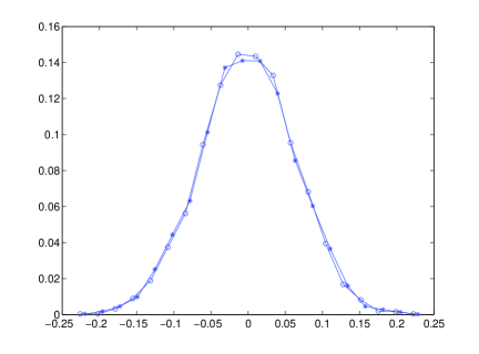
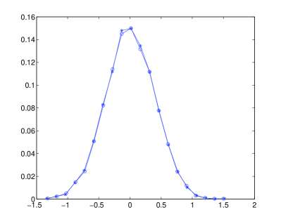
Figure 1: Empirical densities of the quantities $\hat{\theta}_{HL}$ (’*’) and $\bar{X}_{n}$ (’o’) for the ARFIMA$(1,d,0)$ model with $d=0.1$ (left), $d=0.35$ (right), $n=600$ without outliers.

Figure 2 displays the same quantities as in Figure 1 when $X_{t}$ has outliers with $d=0.1$ (left) and $d=0.35$ (right). As expected, the sample mean is much more sensitive to the presence of outliers than the Hodges-Lehmann estimator. Observe that when the long-range dependence is strong (large $d$), the effect of outliers is less pronounced.

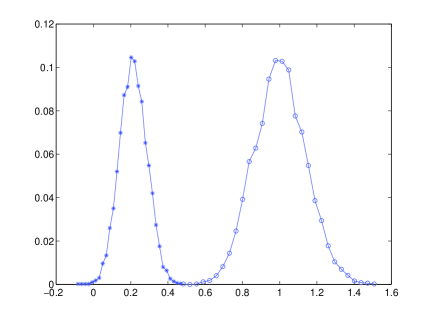
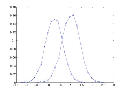
Figure 2: Empirical densities of the quantities $\hat{\theta}_{HL}$ (’*’) and $\bar{X}_{n}$ (’o’) for the ARFIMA$(1,d,0)$ model with $d=0.1$ (left), $d=0.35$ (right), $n=600$ with outliers ($p=10\%$ and $\omega=10$).

6.2 Shamos scale estimator

In this section, we illustrate the results of Proposition 8. In Figure 3, the empirical densities of $\hat{\sigma}_{BL}-\sigma$ and $\hat{\sigma}_{n,X}-\sigma$ are displayed when $d=0.1$ without outliers (left) and with outliers (right). In the left part of this figure, we illustrate the results of the first part of Proposition 8 since both shapes are similar to that of Gaussian density with mean zero. On the right part of Figure 3, we can see that the classical scale estimator is much more sensitive to the presence of outliers than the Shamos-Bickel estimator.

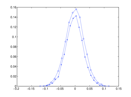
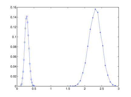
Figure 3: Empirical densities of the quantities $(\hat{\sigma}_{BL}-\sigma)$ (’*’) and $(\hat{\sigma}_{n,X}-\sigma)$ (’o’) for the ARFIMA$(1,d,0)$ model with $d=0.1$, $n=600$ without outliers (left) and with outliers $p=10\%$ and $\omega=10$ (right).

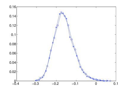
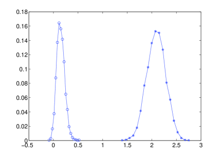
Figure 4: Empirical densities of the quantities $(\hat{\sigma}_{SB}-\sigma)$ (’*’) and $(\hat{\sigma}_{n,X}-\sigma)$ (’o’) for the ARFIMA$(1,d,0)$ model with $d=0.35$, $n=600$ without outliers (left) and with outliers $p=10\%$ and $\omega=10$ (right).

Figure 4 (left) illustrates the second part of Proposition 8. $d=0.35$ corresponds to $D=0.3<1/2$. The right part of Figure 4 shows the robustness of the Shamos estimator with respect to the classical scale estimator in the presence of outliers.

References

- Arcones (1994) {barticle}[author] \bauthor\bsnmArcones, \bfnmM.A.\binitsM. (\byear1994). \btitleLimit theorems for nonlinear functionals of a stationary Gaussian sequence of vectors. \bjournalAnnals of Probability \bvolume22 \bpages2242–2274. \endbibitem
- Beran (1991) {barticle}[author] \bauthor\bsnmBeran, \bfnmJ.\binitsJ. (\byear1991). \btitle Estimators of Location for Gaussian and Related Processes With Slowly Decaying Serial Correlations. \bjournalJournal of the American Statistical Association \bvolume86 \bpages704–708. \endbibitem