Non-Gaussian Fingerprints of Self-Interacting Curvaton
Abstract:
We investigate non-Gaussianities in self-interacting curvaton models treating both renormalizable and non-renormalizable polynomial interactions. We scan the parameter space systematically and compute numerically the non-linearity parameters and . We find that even in the interaction dominated regime there are large regions consistent with current observable bounds. Whenever the interactions dominate, we discover significant deviations from the relations and valid for quadratic curvaton potentials, where measures the curvaton contribution to the total energy density at the time of its decay. Even if , there always exists regions with since the sign of oscillates as a function of the parameters. While can also change sign, typically is non-zero in the low- regions. Hence, for some parameters the non-Gaussian statistics is dominated by rather than by . Due to self-interactions, both the relative signs of and and the functional relation between them is typically modified from the quadratic case, offering a possible experimental test of the curvaton interactions.
HD-THEP-09-32
1 Introduction
In the curvaton scenario [1], primordial perturbations originate from quantum fluctuations of a curvaton field which remains effectively massless during inflation and contributes very little to the total energy density. After the end of inflation, the curvaton energy density stays nearly constant until the field becomes effectively massive, while the dominating radiation component generated at reheating scales as . The curvaton contribution to the total energy density therefore grows rapidly after the end of inflation and its perturbations start to affect the expansion history. In this way the initial isocurvature fluctuations of the curvaton field get gradually converted into adiabatic curvature perturbations. The observed primordial perturbation can originate solely from the curvaton perturbations, although scenarios with mixed inflaton and curvaton perturbations are also possible [2]. As the curvaton finally decays and the decay products thermalize, the adiabatic hot big bang epoch is recovered and the curvature perturbation freezes to a constant value on superhorizon scales.
Predictions of the curvaton scenario depend crucially on the form of the curvaton potential [3, 4, 5, 6, 7, 8, 9, 10, 11] (and the background evolution [12]). Although the curvaton must be weakly coupled to the thermal bath after the end of inflation, interactions of some type should be present in realistic models.
In the present paper, we consider self-interacting curvaton models with the generic potential
| (1) |
with and . We set throughout the paper. In [10] it was found numerically that the predictions of such models can deviate significantly from the extensively studied quadratic case [13], as shown already in [4, 5] in the limit of small interactions. For non-quadratic potentials the amplification of curvaton energy after inflation is less efficient than in the quadratic case, but one may still generate the observed amplitude of primordial perturbation since the curvaton perturbation generated during inflation, , can be larger than . As shown in [10], the correct amplitude can be achieved in a relatively large part of the parameter space.
However, the dynamics is very complicated and, for non-renormalizable potentials, the curvature perturbation (here understood to contain all orders of perturbation theory) displays oscillations as a function of the initial curvaton field value . This reflects the dynamics of transition from curvaton oscillations in the non-quadratic part of the potential to the quadratic part, as discussed in [10]. For the (marginally) renormalizable case, , the transition does not give rise to an oscillatory behaviour of but nevertheless affects the final value of the perturbation.
Here we extend the analysis of [10] and focus on primordial non-Gaussianities generated in the class of curvaton models with the potential (1). We use the formalism and solve the equations of motion numerically. We perform a systematic scan through the parameter space and evaluate the non-linearity parameters and . Combining this information with the amplitude of perturbations, we find the regions of the parameter space that are consistent with current observational constraints. As a result of the oscillatory behaviour of , the observational constraints on the self-interacting model (1) differ significantly from the quadratic case.
The paper is organized as follows. In Sect. 2 we give our basic definitions and discuss the generic features of the non-linearity parameters and . In Sect. 3, we tackle the special case of the renormalizable, four point interaction, for which we can use the analytical estimates derived in [10]. In Sect. 4, we extend our analysis to non-renormalizable interactions with by resorting to numerics. This section contains our main results. Finally, in Sect. 5 we present our conclusions.
2 Non-Gaussianities in self-interacting curvaton models
We use the formalism [14, 15] and assume that the curvature perturbation arises solely from perturbations of a single curvaton field generated during inflation. The curvature perturbation can then be expanded as
| (2) |
Here is the number of e-foldings from an initial spatially flat hypersurface with fixed scale factor to a final hypersurface with fixed energy density , evaluated using the FRW background equations. The final time should be chosen as some (arbitrary) time event after the curvaton decay. The prime denotes a derivative with respect to the initial curvaton value . Here we take to be some time during inflation soon after all the cosmologically relevant modes have exited the horizon and assume the curvaton perturbations are Gaussian at this point. The expansion (2) is then of the form
| (3) |
where is a Gaussian field and the non-linearity parameters are given by
| (4) | |||||
| (5) |
Here we neglect all the scale dependence of the non-linearity parameters [16]. With this assumption and neglecting higher order perturbative corrections, the constants and measure the amplitudes of the three- and four-point correlators of respectively.
We assume the curvaton obeys slow roll dynamics during inflation and introduce a parameter to measure its contribution to the total energy density at
| (6) |
The inflationary scale appears as a free parameter in our analysis, up to certain model dependent consistency conditions. Assuming inflation is driven by a slowly rolling inflaton field, we need to require in order to make the inflaton contribution to negligible. In this setup we also need to adjust , determined by the inflaton dynamics, to give the correct spectral index, [17]. The curvaton contribution, , is typically negligible because of the subdominance of the curvaton. The curvaton mass needs to be small but the same also holds for the inflaton mass. We assume this minimal setup in the current work for definiteness since our main goal is to discuss the new features arising from curvaton self-interactions.
After the end of inflation, we assume the inflaton decays completely into radiation and the universe becomes radiation dominated. We introduce a phenomenological decay constant to account for the coupling between the radiation and the curvaton component. The evolution of the coupled system is given by
| (7) | |||||
| (9) | |||||
The initial conditions are given by and specified at time corresponding to the end of inflation. We also put . Given the parameters , and , which determine the potential (1), and the two initial conditions and , we can calculate in (2) from this set of equations. To find the curvature perturbation, we set and compute . For a given set of parameters, we adjust the decay width so that the observed amplitude is obtained, [18].
We treat as a free parameter since we have not specified the curvaton couplings to other matter, in particular to the Standard Model fields. However, since the primordial perturbations have been observed to be adiabatic to a high degree [18], the curvaton should decay before dark matter decouples in order not to produce isocurvature modes. Assuming the freeze-out temperature for an LSP type dark matter model with GeV, this translates to a rough bound
| (10) |
While this bound could be relaxed in non-minimal constructions, we assume it for definiteness for the rest of our work.
2.1 Analytical considerations
In Sect. 4 we solve the set of equations (7) - (9) numerically and compute the resulting curvature perturbation (2) and the non-linearity parameters (4) and (5). However to gain some physical insight of the results, it is useful to start by discussing generic approximative analytic expressions that can be derived for and . Assuming the curvaton decays instantaneously [19] at and neglecting the coupling between curvaton and radiation before , one can can estimate the non-linearity parameters by [5, 20, 21]
| (11) | |||||
Here and is the envelope of the oscillating curvaton field at some time after the beginning of oscillations in the quadratic part of the potential. The results are independent of the precise choice of .
If the curvaton potential is exactly quadratic, and the non-linearity parameters and are uniquely determined by , i.e. by the curvaton energy density at the time of decay. However, interactions in general make the function non-linear and, especially in the limit , the quadratic predictions can be greatly altered due to the derivative terms in (11) and (2.1). If the interactions dominate the curvaton dynamics at the time of inflation, the non-linearity parameters can only very crudely be approximated by and . As will be discussed in Sect. 4, in the interacting case the non-linearity parameters can deviate significantly from these naïve estimates. This follows from the non-trivial behaviour of derivatives of in (11) and (2.1).
In particular, we find that for in the potential (1) the signs of the non-linearity parameters and oscillate as a function of . Therefore, even if , it is always possible to find regions where the non-Gaussianities are accidentally suppressed and do not conflict current observational bounds. For example, from (11) we see that for whenever . Using the definitions (4) and (5) we find,
| (13) |
which gives an estimate for the typical size of the regions . This is larger than the range of field values probed by the curvaton fluctuations produced during inflation, , if . Therefore, for we may conclude that the regions correspond to a self-consistent choice of initial conditions and are not destabilized by the fluctuations produced during inflation.
3 Renormalizable potential
The special case of a quartic interaction term in the potential,
| (14) |
can be discussed using the analytical estimates presented in [10]. If the interaction dominates over the quadratic term at the time of inflation, the curvaton oscillations start in an effectively quartic potential. As the amplitude of the oscillating field decreases, the quartic term dilutes away and the potential becomes quadratic. Assuming the universe remains radiation dominated until the curvaton decay, , the envelope of the oscillating curvaton in the quadratic regime is given by
| (15) |
The function can be estimated using Eq. (4.9) in [10], which assumes and is derived to leading order precision in . In approaching the quadratic limit, , the analytical estimates of [10] can no longer be used to obtain quantitative results but the qualitative features remain correct.
To leading order in , Eqs. (11) and (2.1) read
| (16) | |||||
| (17) |
and by substituting (15) into these, we find (semi)analytical predictions for and . The results are illustrated in Fig. (1).
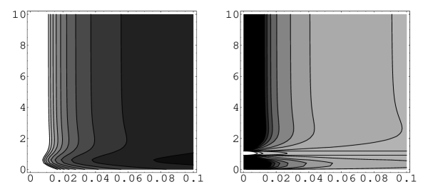
Although the case does not result into oscillatory behaviour of , non-monotonous features appear when considering derivatives of , i.e. the coefficients etc. in (2). These features become the more pronounced the higher the order of the derivative is. This can also be observed in Fig. (1) where both and display non-monotonous behaviour as a function of in the region . For the non-monotonous features are very mild but shows a significantly more sensitive dependence on .
As discussed in [10], for the transition from the quartic to the quadratic part of the potential takes place soon after the onset of oscillations when and still act as independent degrees of freedom. These quantities in general do not have a similar dependence on the initial field value . Variations of therefore affect the effective equation of state of the oscillating curvaton in a non-trivial fashion and this is the origin of the structure seen in Fig. (1). If or , no similar structure is seen. In the former case, the transition into quadratic region happens when the dynamics of the oscillating curvaton is already well described by a single dynamical degree of freedom, the amplitude . In the latter case the potential is almost Gaussian from the beginning.
4 Non-renormalizable potentials
The discussion in the preceding section, together with the oscillatory behaviour of presented in [10], leads to an expectation that for non-renormalizable curvaton potentials the naiïve estimates and can be violated for a range in the parameter space. It is however not obvious at all how large this range might be. Since the analtyical approximations used in the previous section cannot be applied to non-renormalizable potentials, we use numerical methods to track the dynamics at hand.
To calculate the values of and for the non-quartic cases, we use code developed for [10] to compute the values numerically using Eqs. 4 and 5. To obtain the derivatives, we calculate for five different initial conditions separated by a spacing , and then use five-point stencil to calculate the first, the second and the third derivative of . We adjust the stepping so that numerical noise is minimized. Furthermore, we adjust for each pixel independently.
4.1 Qualitative features and differences from naïve expectations
For all choices of and , the parameter space is divided into two areas by a line where the quadratic and the non-quadratic terms are equal for the initial curvaton field value, i.e.,
Below this quadratic line we should recover the behaviour predicted analytically for the quadratic case. Above this line the self-interactions modify the behaviour substantially.
For case the behaviour in the non-quadratic regime is smooth and qualitatively in close resemblance with the case , which was described in the previous section. This is due to the fact that if , the field does not oscillate in the non-renormalizable part of the potential at all. However, for the cases and large oscillations of as a function of its parameters and initial conditions are present in the non-quadratic regime as described in [10]. Here the expressions and provide only very rough estimates of the non-linearity parameters, and in the interaction dominated region the actual values of and can deviate significantly from these estimates. This behaviour can be traced back to the terms including derivatives of in the Eqs. (11) and (2.1).
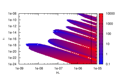
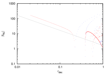
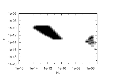
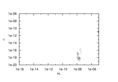
In Fig. 2(a) we have plotted the value of against the initial conditions and . The vertical line in this figure corresponds to a range of parameters, corresponding to the fixed value of , for which is plotted against in Fig. 2(b). Here can be seen oscillating around the -estimate. Oscillations arise from the derivative terms present in Eq. (11), which describe the impact of the self-interaction terms on the dynamics of the curvaton. Most points give rise to a larger than one would expect from the estimate , however since actually changes sign, points can always be found where is arbitrarily close to zero. In Fig. 2(b) several different values of correspond to a given point since different choices of initial conditions can be degenerate yielding the same .
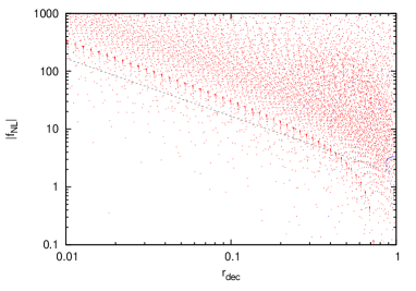
In Fig. 2(c) we plot again against , but we no longer constrain , but instead plot this for all points in Fig. 2(a). Again each point corresponds to a set of parameters producing the observed final amplitude of the primordial perturbations. As we allow to take different values, a family of curves is drawn, where each curve is similar to the curve present in 2(b), resulting into the noisy scatter present in the Fig. 2(c). It is also noteworthy that for given fixed value of , there are multiple sets of parameters which all give the same final amplitude for the perturbations, but different value of (and ).
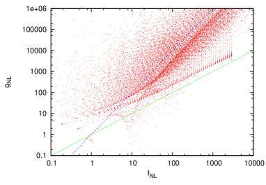
In Fig. 2(d) the value of is plotted against . Here three contributions can be clearly distinguished: The -relation arising while in the quadratic regime, the -relation in the non-quadratic regime that is due to self-interactions, and scatter around those lines due to the oscillations caused by the self-interactions. This scatter can be understood by considering Fig. 2(b) where can be seen oscillating around the analytical estimate. Plotting against would produce a qualitatively similar plot as Fig. 2(b) showing the oscillations around the and estimates deriving from the terms in eq. (11). However, in general and do not oscillate with the same phase, and hence when plotting against , scatter is created.

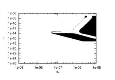
In Fig. 3(a) - 3(d) the magnitudes and signs of and are plotted when scanned through different initial conditions. Here again the oscillatory features can be clearly distinguihed as both and oscillate in the regime initially dominated by the non-quadratic interaction. Moreover it is worth emphasizing that not only does the absolute magnitude of and show oscillatory behaviour in this regime, but also their signs change along the oscillations as shown in Fig. 3(b) and 3(d). Futhermore the oscillations of and have different periods and phases, i.e. the zeros of and are not related in a simple fashion.
In Eq. (13) we presented a relation between the derivative of with respect to and the values of and . If , this takes a particularly simple form, , which can be clearly seen in Fig. 3(c).
Note that there are two different sources of non-Gaussianity: one is the subdominance of the curvaton at the time of decay , while the other is just the non-linear evolution of curvaton perturbations, encoded in the function in Eqs. (11) and (2.1). Even if , large non-Gaussianity can be generated by the evolution of the curvaton. For example, from Eq. (11) we see that if , can be very large even though . This can be understood qualitatively by looking at the expression for the linear part of the curvature perturbation, [20]. If , we see that we need to increase to keep . Therefore, the higher order terms become significant in this limit generating large non-Gaussianities, just like in the limit .
4.2 Allowed regions of parameter space
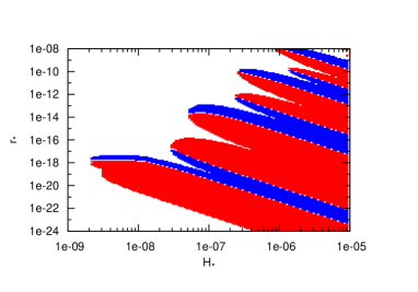
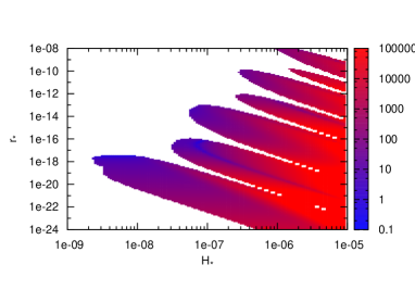
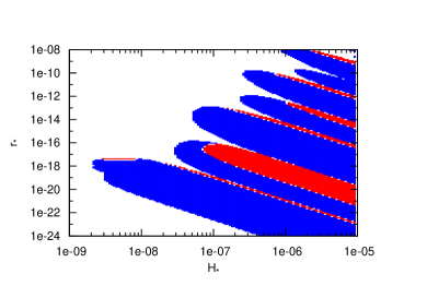
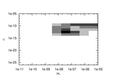
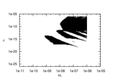
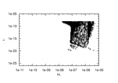
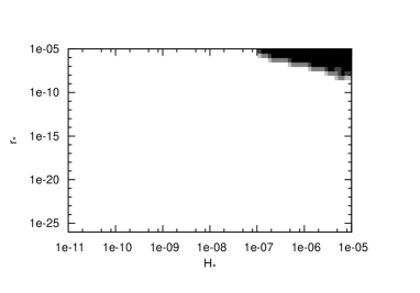
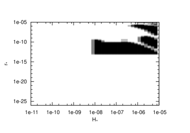
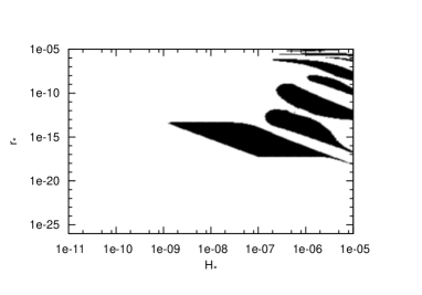
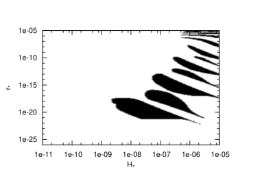
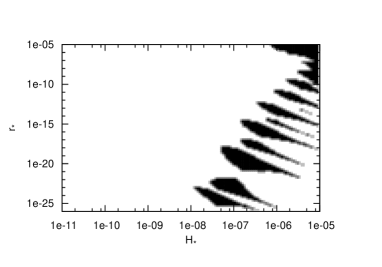
In Figs. 5 - 7 we have plotted the points in the parameter space which are compatible with observations of the primordial perturbations. These points give rise to the observed amplitude of the perturbations while producing and which are within the current observable limits.
The range of the initial conditions and has been chosen so that all interesting features should be within the plots. is also bounded from above, , to prevent the excessive production of primordial tensor modes and at least an order of magnitude smaller to keep the inflaton perturbations negligible.
Limits for are given by the WMAP 5-year data [18], . Although in [23] a more stringent constraint for is given as , we conservatively use the limit provided in [18]. Regarding the limits for , we require that is the range as given in [24]. Note that these limits have been derived assuming , which here is not the case in general. However, the bounds for seem to be much more constraining in our case, and relaxing the limits for even by an order of magnitude would not enlarge the allowed area of the parameter space significantly. Thus we adopt this limit for reference purposes555 Recently, the authors of [25] have obtained limits on without assuming by using N-point probability distribution function. However, their constraint on is similar to that of [24]..
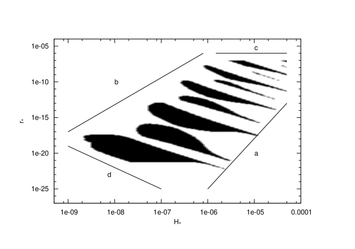
In Fig. 4 we give an illustration of the different features limiting the allowed area of the parameter space. The observational limits for and constrain the allowed area in the very subdominant regions of the parameter space, as depicted in Fig. 4 by the line a. Other constraints shown in Fig. 4 arise from the internal consistency of the specific curvaton scenario studied in the present paper. The bound b is obtained because otherwise the initial perturbations would be too small to produce the observed amplitude. The bound c reflects the requirement that the curvaton should be massless, or , which is necessary for the generation of curvaton perturbations during inflation. Because of the subdominance of the curvaton, the realistic bound should arguably be a few orders of magnitude tighter. However, a change of an order of magnitude moves the actual cut by a very small amount in the log-log plots.
Finally, the bound d guarantees the absence of the isocurvature modes in dark matter perturbations and corresponds to the limit on the curvaton decay width given in (10).
It should be noted, that limits b, c and d in Fig. 4 were already present in [10], so that the non-Gaussianty limit a is the only new limiting ingredient provided by the current work on the space of parameters.
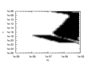
As explained in the previous sections, in the regions where the quadratic part of the potential dominates already initially, the dynamics are essentially linear, and the simple results apply. As a consequence, dependence in Eqs. (11) and (2.1) disappears. Therefore these regions are characterized by the smooth continuous allowed area as shown in Figs. 5 - 7, which can be found in the lower left are in the plots. The total area of the allowed region depends on the values of and ; e.g. for and this quadratic area is much larger than for, say, and .
As mentioned previously, and do not display extended oscillatory regions. Hence the plots in Fig. 5 remain smooth also in the regime where the self-interaction dominates.
The cases and are however characterized by significant oscillatory features, as discussed in the previous sections. Due to these oscillations, the allowed region consists of isolated patches in the interaction dominated regime. As can be seen in the figures, the size of these patches decreases as we decrease the (bare) mass , since this tends to make the curvaton more subdominant at the time of decay, decreasing the viable area.
5 Discussion
It seems plausible that the curvaton, like any other scalar field, has some self-interactions. These self-interactions can have a profound effect on the dynamical evolution of the curvaton field and its perturbations, as was discussed in [10] (and in [4, 5])), where we studied the amplitude of the curvature perturbation in self-interacting curvaton models defined by Eq. (1). In the present paper we have focussed on the non-Gaussianities of the curvature perturbations by computing the non-linearity parameters and for all the model parameters for which .
When the curvaton has some self-interactions, the non-Gaussian statistics of the curvature perturbation can be quite different from that produced in the simplest model with a quadratic potential. In the quadratic curvaton model, the magnitude of in the limit is determined by the curvaton energy density at the time of its decay, . However, the prediction of can significantly deviate from this simple estimate if the curvaton has non-renormalizable self-interactions. As seen from Fig. 2(c), for such models the values of scatter around the estimate and typically end up being slightly larger than in the quadratic case. Thus a very subdominant curvaton is not favoured because it tends to yield a value of which is in excess of the observational bounds [18, 23].
However, it is interesting to note that even if , there exists regions in the parameter space with . This is because the value of oscillates and changes its sign, as is illustrated in Fig. 2(a) for . However, even if , the non-linearity parameter for the trispectrum can be very large, as can be seen in Fig. 2(d). In these regions the self-interacting curvaton scenario gives rise to a rather non-trivial non-Gaussian statistics characterized by a large trispectrum and a vanishing bispectrum. Such a situation, discussed already in [5], appears to be rather generic in self-interacting curvaton models, and possible for a wide, albeit restricted, range of model parameters.
Another interesting feature of the curvaton model with self-interactions is that large non-Gaussianities can be generated even if the curvaton dominates the energy density at the time of its decay, . Recently in [26] it was shown that for , the entropy production at the curvaton decay can leave an imprint on the spectrum of primordial graviational waves, which in principle could be observable. If the curvaton had no self-interactions, such a signal would imply that no large non-Gaussianity could be generated by the curvaton fluctuations. This is clearly not the case when the self-interactions are included, which serves to demonstrate thet the self-interactions can significantly affect the generic features of the curvaton scenario.
Another interesting feature that is clearly visible in Fig. 2(d) is the breakdown of the relation of which holds true for the quadratic potential. For the self-interacting curvaton a large number of points, each corresponding to an allowed set of parameter values, can be seen to fall into the region with . If the interactions are small compared to the quadratic part, the linear relation gets replaced by [5]. However, when the self-interaction term dominates, both of the above relations can be violated, as is seen from Fig. 2(d). There is nevertheless a tendency for the points to be concentrated around the lines and .
We should also like to point out that in the quadratic case with , the signs of and are respectively positive and negative. In contrast, in the cases studied here, the signs can well be the same. This feature provides an obvious departure from the quadratic case and could offer an experimental possibility to constrain the curvaton self-interaction.
It is evident from the figures presented in Sect. 4 that the self-interacting curvaton model provides us a rich tapestry of features, constrained in a highly non-trivial way by the observational limits on non-Gaussianity. As we have argued here, in the presence of self-interactions the relative signs of and and the functional relation between them is typically modified from the quadratic case. Thus the non-linearity parameters taken together, in possible conjunction of other cosmological observables such as tensor perturbations, may offer the best prospects for constraining the physical properties of the curvaton.
Acknowledgments.
This work is supported in part by the Grant-in-Aid for Scientific Research from the Ministry of Education, Science, Sports, and Culture of Japan No. 19740145 (T.T.), by the EU 6th Framework Marie Curie Research and Training network ”UniverseNet” (MRTN-CT-2006-035863), by the Academy of Finland grants 114419 (K.E.) and 130265 (S.N.) and by the Magnus Ehrnrooth Foundation (O.T.).References
- [1] K. Enqvist and M. S. Sloth, Nucl. Phys. B 626, 395 (2002) [arXiv:hep-ph/0109214]; D. H. Lyth and D. Wands, Phys. Lett. B 524, 5 (2002) [arXiv:hep-ph/0110002]; T. Moroi and T. Takahashi, Phys. Lett. B 522, 215 (2001) [Erratum-ibid. B 539, 303 (2002)] [arXiv:hep-ph/0110096]; A. D. Linde and V. F. Mukhanov, Phys. Rev. D 56 (1997) 535 [arXiv:astro-ph/9610219]; S. Mollerach, Phys. Rev. D 42 (1990) 313.
- [2] D. Langlois and F. Vernizzi, Phys. Rev. D 70 (2004) 063522 [arXiv:astro-ph/0403258]; G. Lazarides, R. R. de Austri and R. Trotta, Phys. Rev. D 70 (2004) 123527 [arXiv:hep-ph/0409335]; F. Ferrer, S. Rasanen and J. Valiviita, JCAP 0410 (2004) 010 [arXiv:astro-ph/0407300]; T. Moroi, T. Takahashi and Y. Toyoda, Phys. Rev. D 72, 023502 (2005) [arXiv:hep-ph/0501007]; T. Moroi and T. Takahashi, Phys. Rev. D 72, 023505 (2005) [arXiv:astro-ph/0505339]; K. Ichikawa, T. Suyama, T. Takahashi and M. Yamaguchi, Phys. Rev. D 78, 023513 (2008) [arXiv:0802.4138 [astro-ph]]; D. Langlois, F. Vernizzi and D. Wands, JCAP 0812 (2008) 004 [arXiv:0809.4646 [astro-ph]].
- [3] K. Dimopoulos, G. Lazarides, D. Lyth and R. Ruiz de Austri, Phys. Rev. D 68 (2003) 123515 [arXiv:hep-ph/0308015].
- [4] K. Enqvist and S. Nurmi, JCAP 0510, 013 (2005) [arXiv:astro-ph/0508573].
- [5] K. Enqvist and T. Takahashi, JCAP 0809, 012 (2008) [arXiv:0807.3069 [astro-ph]].
- [6] K. Enqvist, S. Nurmi and G. I. Rigopoulos, JCAP 0810 (2008) 013 [arXiv:0807.0382 [astro-ph]].
- [7] Q. G. Huang, JCAP 0811, 005 (2008) [arXiv:0808.1793 [hep-th]].
- [8] M. Kawasaki, K. Nakayama and F. Takahashi, JCAP 0901, 026 (2009) [arXiv:0810.1585 [hep-ph]].
- [9] P. Chingangbam and Q. G. Huang, JCAP 0904, 031 (2009) [arXiv:0902.2619 [astro-ph.CO]].
- [10] K. Enqvist, S. Nurmi, G. Rigopoulos, O. Taanila and T. Takahashi, JCAP 0911, 003 (2009) [arXiv:0906.3126 [astro-ph.CO]].
- [11] A. Chambers, S. Nurmi and A. Rajantie, arXiv:0909.4535 [astro-ph.CO].
- [12] K. Enqvist and T. Takahashi, JCAP 0912, 001 (2009) [arXiv:0909.5362 [astro-ph.CO]].
- [13] D. H. Lyth, C. Ungarelli and D. Wands, Phys. Rev. D 67, 023503 (2003) [arXiv:astro-ph/0208055].
- [14] A. A. Starobinsky, JETP Lett. 42 (1985) 152 [Pisma Zh. Eksp. Teor. Fiz. 42 (1985) 124]; M. Sasaki and E. D. Stewart, Prog. Theor. Phys. 95, 71 (1996); M. Sasaki and T. Tanaka, Prog. Theor. Phys. 99, 763 (1998).
- [15] D. Wands, K. A. Malik, D. H. Lyth and A. R. Liddle, Phys. Rev. D 62 (2000) 043527 [arXiv:astro-ph/0003278]; D. H. Lyth and D. Wands, Phys. Rev. D 68, 103515 (2003) [arXiv:astro-ph/0306498]; D. H. Lyth, K. A. Malik and M. Sasaki, JCAP 0505, 004 (2005);
- [16] C. T. Byrnes, S. Nurmi, G. Tasinato and D. Wands, arXiv:0911.2780 [astro-ph.CO].
- [17] D. Wands, N. Bartolo, S. Matarrese and A. Riotto, Phys. Rev. D 66 (2002) 043520 [arXiv:astro-ph/0205253].
- [18] E. Komatsu et al. [WMAP Collaboration], Astrophys. J. Suppl. 180, 330 (2009) [arXiv:0803.0547 [astro-ph]].
- [19] K. A. Malik, D. Wands and C. Ungarelli, fluids,” Phys. Rev. D 67 (2003) 063516 [arXiv:astro-ph/0211602].
- [20] D. H. Lyth and Y. Rodriguez, Phys. Rev. Lett. 95 (2005) 121302 [arXiv:astro-ph/0504045].
- [21] M. Sasaki, J. Valiviita and D. Wands, Phys. Rev. D 74, 103003 (2006) [arXiv:astro-ph/0607627].
- [22] M. S. Turner, Phys. Rev. D 28 (1983) 1243.
- [23] K. M. Smith, L. Senatore and M. Zaldarriaga, JCAP 0909, 006 (2009) [arXiv:0901.2572 [astro-ph]].
- [24] V. Desjacques and U. Seljak, arXiv:0907.2257 [astro-ph.CO].
- [25] P. Vielva and J. L. Sanz, arXiv:0910.3196 [astro-ph.CO].
- [26] K. Nakayama and J. Yokoyama, arXiv:0910.0715 [astro-ph.CO].