Decoherence and Entanglement Dynamics in Fluctuating Fields

Abstract

We study pure phase damping of two qubits due to fluctuating fields. As frequently employed, decoherence is thus described in terms of random unitary (RU) dynamics, that is, a convex mixture of unitary transformations. Based on a separation of the dynamics into an average Hamiltonian and a noise channel, we are able to analytically determine the evolution of both entanglement and purity. This enables us to characterize the dynamics in a concurrence-purity (CP) diagram: We find that RU phase-damping dynamics sets constraints on accessible regions in the CP plane. We show that initial state and dynamics contribute to final entanglement independently.

I Introduction

For newly emerging quantum technologies, robustness of quantum states is essential. In particular, stability of entanglement spread over a many-body quantum system is of fundamental importance for quantum cryptography and quantum information processing in general. A thorough understanding of processes known to destroy the desired quantum qualities—usually subsumed under the name of decoherence—is necessary. Phase damping represents the case of pure decoherence, where coherences of a given state in a certain basis are subject to decay while probabilities, that is diagonal elements of the density matrix, remain unchanged. It is well known that despite the rather simple nature of phase damping, it is clearly enough to disentangle quantum states Yu2003 ; Mintert2005 .

A widely encountered source of decoherence is growing entanglement between a quantum system and its environment. Yet, often decoherence is due to—or at least may be explained in terms of—random unitary (RU) dynamics. Then, fluctuating classical fields are liable for the loss of quantum properties (sometimes also termed “random external fields”) AlickiLendi ; NielsenChuang . Although it is known that RU dynamics is not the most general form of decoherence LandauStreater ; HelmStrunz , it is of great practical importance. For instance, in quantum computers based on trapped ions, these classical fluctuations are believed to be the main source of decoherence Monz2009 . Here, fluctuations are present both in the magnetic field of the trap and in the frequency of the laser addressing the qubits. RU dynamics moreover serves as a model to introduce decoherence in experiments in a controlled fashion Myatt2000 . In the context of quantum error correction, RU processes are of special interest, because they represent the only type of errors that may be completely undone GregorattiWerner . The present work will further reveal how decoherence of qubits due to RU dynamics allows for a surprisingly far-reaching analytical treatment.

For a system of two qubits a possible means of characterization relies upon the relation between entanglement and entropy Ishizaka2000 ; Ziman2005 . The system’s state $\varrho$ may be studied in terms of a CP diagram, where entanglement (here measured through concurrence $C$) is plotted against purity, $P(\varrho)=\mbox{tr}(\varrho^{2})$, a common measure for the mixedness of $\varrho$. This approach has been used in several theoretical studies, where Bell states subject to single-sided dynamics Ziman2005 (by single-sided dynamics we denote the case where only one part of a bipartite system is affected), decoherence in a random matrix environment Pineda2007 , or two interacting atoms in a cavity Torres2009 were considered.

It was noted earlier that decoherence in ion trap quantum computers is not of simple exponential type Schmidt-Kaler2003 , as would be expected from a Markovian master equation approach. A theoretical model incorporating this fact thus calls for a more general treatment. From an axiomatic point of view (neglecting initial correlations) the dynamics of a quantum system is given in terms of completely positive maps (or quantum channels) NielsenChuang . In a Hilbert space of dimension $d$, these channels can always be written in terms of at most $d^{2}$ Kraus operators $K_{i}$ such that

$$\varrho\mapsto\varrho^{\prime}=\mathcal{E}[\varrho]=\sum_{i}K_{i}\varrho K_{i}^{\dagger}$$ (1)

(throughout the article we denote the initial state by $\varrho$ and its map by $\varrho^{\prime}$). For RU channels there exists an expression of the form (1) where every Kraus operator is proportional to some unitary operator, so that the dynamics is a convex combination of unitary transformations: $\varrho^{\prime}=\sum_{i}p_{i}U_{i}\varrho U_{i}^{\dagger}$, with $p_{i}>0$ and $\sum_{i}p_{i}=1$. Phase-damping channels stand out due to the requirement to be diagonal in the distinguished basis, that is, they may be written in the form

$$\varrho^{\prime}_{mn}=\langle a_{n}|a_{m}\rangle\varrho_{mn}=:D_{mn}\varrho_{mn},$$ (2)

with $\{\left|a_{n}\right\rangle\}$ any set of $d$ normalized complex vectors Havel ; Paulsen . In “system plus environment” models, the vectors $|a_{n}\rangle$ may be identified with environmental quantum states GorinStrunz2004 . For RU phase damping, a simple interpretation of the $|a_{n}\rangle$ is less obvious.

In this article we study RU phase damping of two qubits. A fully analytical expression for both the entanglement evolution and the purity decay is obtained. Throughout the article the initial two-qubit state is assumed to be pure. The phase damping will be realized as an ensemble average $\left\langle\!\left\langle U(t)\varrho U^{\dagger}(t)\right\rangle\!\right\rangle$, where the unitary (diagonal) time evolution may be regarded as arising from a stochastic Hamiltonian of the form

$$H(t)=\omega_{1}(t)\sigma_{z}^{A}\otimes\mathds{1}+\omega_{2}(t)\mathds{1}\otimes\sigma_{z}^{B}+\omega_{3}(t)\sigma_{z}^{A}\otimes\sigma_{z}^{B}.$$ (3)

With $\sigma_{z}$ we denote the diagonal Pauli spin operators for qubits $A$ and $B$, respectively, the time dependence is due to the stochastic processes $\omega_{1}(t),\omega_{2}(t)$, and $\omega_{3}(t)$. In an experimental realization using two-state atoms this would correspond, for example, to a fluctuation of the individual Zeeman levels described by $\omega_{1}(t)$ and $\omega_{2}(t)$, together with an instability in the interaction of the atom’s energy eigenstates, described by $\omega_{3}(t)$. Such a Hamiltonian is used to describe the spin-spin interaction in nuclear magnetic resonance (NMR) systems Vandersypen2004 . Also note that the third term of Eq. (3) describing the interaction—later referred to as pure two-qubit phase damping—is implemented in the realization of a phase gate in recent ion trap experiments Monz2009 .

Recently, for a quantum system subject to single-sided dynamics a very simple evolution equation for entanglement was found Konrad2007 . This evolution equation allows for a factorization into a functional characterizing the quantum channel and the amount of the initial pure-state entanglement. In our case here, the evolution will in general be nonlocal. Yet, we are also able to give some exact evolution equations for entanglement under phase damping, where the channel and the initial state enter independently.

The article is organized as follows: In Sec. II we discuss our model of RU phase damping, where we benefit from a separation of the channel into a reversible part due to a mean Hamiltonian and an irreversible noise channel. This separation enables us to analytically study changes in entanglement and purity. In Sec. III we discuss RU single-qubit channels in the context of the CP diagram. Here we are able to give an alternative explanation of the results obtained in Ref. Ziman2005 , where for a maximally entangled state subject to unital (mapping the completely mixed state onto itself) single-sided channels certain bounds to the accessible area within the CP diagram were found. Our approach, which employs the so-called Jamiolkowski isomorphism, will also be well suited for explaining part of the findings at hand. In Secs. IV and V we analyze in detail the evolution of entanglement and purity of a pure separable and a general pure initial state under RU phase damping, respectively.

II RU Phase Damping

The phase damping we consider shall be realized as an ensemble average $\varrho^{\prime}=\left\langle\!\left\langle U(t)\varrho U^{\dagger}(t)\right\rangle\!\right\rangle$, where we may set $U(t)=e^{-i\int_{0}^{t}d\tau H(\tau)}$, a unitary map based on a stochastic diagonal Hamiltonian $H(t)$. As an example let us consider a single-qubit channel, where a generic diagonal Hamiltonian may simply be set to $H(t)=\omega(t)\sigma_{z}$ with some stochastic process $\omega(t)$. Assuming $\omega(t)$ to add up to a total perturbation of the qubit, the central limit theorem tells us that $\Omega:=\int_{0}^{t}d\tau\omega(\tau)$ is a Gaussian random variable that is determined by its mean, $\mu:=\left\langle\!\left\langle\Omega\right\rangle\!\right\rangle$, and its variance, $\sigma^{2}=:\left\langle\!\left\langle\Omega^{2}\right\rangle\!\right\rangle-\mu^{2}$, hence leading to $\left\langle\!\left\langle e^{\pm i\Omega t}\right\rangle\!\right\rangle=e^{\pm i\mu}e^{-\frac{1}{2}\sigma^{2}}$.

Substituting $\mu\rightarrow\theta$ and $\frac{1}{2}(1-e^{-\frac{1}{2}\sigma^{2}})\rightarrow p$, we thus arrive at the most general form of a single-qubit phase-damping channel

$$\varrho^{\prime} = \begin{pmatrix}\varrho_{11}&\left\langle\!\left\langle e^{-i\Omega t}\right\rangle\!\right\rangle\varrho_{12}\\ \left\langle\!\left\langle e^{i\Omega t}\right\rangle\!\right\rangle\varrho_{21}&\varrho_{22}\end{pmatrix}$$

$$= e^{-i\frac{\theta}{2}\sigma_{z}}\left((1-p)\;\varrho+p\;\sigma_{z}\varrho\sigma_{z}\right)e^{i\frac{\theta}{2}\sigma_{z}}.$$

Thus, single-qubit phase damping may always be written in terms of RU dynamics LandauStreater . From our example we see furthermore that it suffices to consider Gaussian fields.

For two qubits the corresponding stochastic diagonal Hamiltonian is

$$H(t)=\omega_{1}(t)\sigma_{z}^{A}\otimes\mathds{1}+\omega_{2}(t)\mathds{1}\otimes\sigma_{z}^{B}+\omega_{3}(t)\sigma_{z}^{A}\otimes\sigma_{z}^{B}.$$

Irrespective of possible correlations among the accumulated phases $\int_{0}^{t}d\tau\omega_{k}(\tau)=:\Omega_{k}$, we find that the phase-damping channel can be decomposed according to

$$\varrho^{\prime} = U_{\mu}(\tilde{D}\star\varrho)U_{\mu}^{\dagger}$$

$$= \tilde{D}\star\left(U_{\mu}\varrho U_{\mu}^{\dagger}\right)$$

into a unitary, reversible part $U_{\mu}$ based on the mean Hamiltonian $H_{\mu}=\mu_{1}\sigma_{z}^{A}\otimes\mathds{1}+\mu_{2}\mathds{1}\otimes\sigma_{z}^{B}+\mu_{3}\sigma_{z}^{A}\otimes\sigma_{z}^{B}$ ($\mu_{k}:=\left\langle\!\left\langle\Omega_{k}\right\rangle\!\right\rangle$) and a nonunitary, irreversible noise channel $\tilde{D}$ (see Appendix A for more details). For brevity of notation we here made use of the Hadamard poduct $\star$ of matrices, that is, the pointwise multiplication of two matrices of the same size HornJohnson .

In close analogy to the single-qubit case we can further deploy the RU phase-damping channel by assuming $\vec{\Omega}$ to be a Gaussian process. It should be noted, however, that our analysis could easily be extended to more general statistics. We can then use the characteristic function Honerkamp

$$\left\langle\!\left\langle e^{\pm i\vec{k}\vec{\Omega}}\right\rangle\!\right\rangle=e^{-\frac{1}{2}\vec{k}^{T}\Sigma\vec{k}\,\pm\,i\vec{k}\vec{\mu}}\quad\forall\vec{k}\in\mathds{C}^{3},$$

where $\vec{\mu}:=\langle\!\langle\vec{\Omega}\rangle\!\rangle$ denotes the mean value, $\Sigma$ is the covariance matrix, and $\Sigma_{kl}:=\langle\!\langle(\Omega_{k}-\mu_{k})(\Omega_{l}-\mu_{l})\rangle\!\rangle$ for a Gaussian process $\vec{\Omega}$.

With no correlations between the stochastic processes $\omega_{1}(t),\omega_{2}(t)$, and $\omega_{3}(t)$, the covariance matrix is diagonal: $\Sigma=\mbox{diag}(2\varsigma_{1}^{2},2\varsigma_{2}^{2},2\varsigma_{3}^{2})$. Note that $\sqrt{2}\varsigma_{k}$ simply denotes the standard deviation of the Gaussian random variable $\Omega_{k}$. The preceding commutativity relation (II) now allows for a separation of the channel into its mixing dynamics and its entangling dynamics: Any change with respect to the purity of the system is due to the noise channel $\tilde{D}$, while any increase in entanglement can only be evoked by (the interaction part of) the mean Hamiltonian $H_{\mu}$. Of course, a decrease in entanglement might as well be due to $\tilde{D}$. However, any gain in entanglement may only be attributed to the unitary map $U_{\mu}$. This separation enables us to calculate changes in purity and concurrence separately.

In order to describe the loss of purity of the system, we need to account for the action of the noise channel, $\tilde{D}$, only,

$$\tilde{D}\star\varrho = p_{1}\varrho+p_{2}(\sigma_{z}^{A}\otimes\sigma_{z}^{B}\;\varrho\;\sigma_{z}^{A}\otimes\sigma_{z}^{B})$$

$$+ \!\!p_{3}(\sigma_{z}^{A}\otimes\mathds{1}\;\varrho\;\sigma_{z}^{A}\otimes\mathds{1})+p_{4}(\mathds{1}\otimes\sigma_{z}^{B}\;\varrho\;\mathds{1}\otimes\sigma_{z}^{B}),$$

where the probabilities $p_{i}$ with $\sum p_{i}=1$ are determined by the variances of the stochastic processes (see Appendix B). The purity for the final state is easily obtained and equates to

$$P(\tilde{D}\star\varrho) = (p_{1}^{2}+p_{2}^{2}+p_{3}^{2}+p_{4}^{2})$$

$$+ 2\big{(}p_{1}p_{3}+p_{2}p_{4}\big{)}\,|\langle\sigma_{z}^{A}\rangle|^{2}$$

$$+ 2\big{(}p_{1}p_{4}+p_{2}p_{3}\big{)}\,|\langle\sigma_{z}^{B}\rangle|^{2}$$

$$+ 2\big{(}p_{1}p_{2}+p_{3}p_{4}\big{)}\,|\langle\sigma_{z}^{A}\otimes\sigma_{z}^{B}\rangle|^{2}.$$

Here and in the following we write $\langle\,\cdot\,\rangle$ for expectation values with respect to the initial state $\left|\psi_{0}\right\rangle$. While the equation for purity decay under RU phase damping is valid irrespective of further details of the initial state, the change in entanglement will be more sensitive to the initial conditions of the two-qubit system. In order to calculate the entanglement created or destroyed in the phase-damping process, we thus need to make some further assumptions about the initial state.

III RU Single-Qubit Channels in the CP Diagram

In the analysis of RU phase damping we want to follow the example of Ref. Ziman2005 , where single-sided unital dynamics was analyzed with respect to entanglement decay as a function of purity decay. The entanglement for a two-qubit system can be easily computed in terms of concurrence, $C(\varrho)=\max\{0,\lambda_{1}-\lambda_{2}-\lambda_{3}-\lambda_{4}\}$, where $\lambda_{1}^{2}\geq\lambda_{2}^{2}\geq\lambda_{3}^{2}\geq\lambda_{4}^{2}$ are the eigenvalues of the positive matrix $R=\varrho\,(\sigma_{y}\otimes\sigma_{y})\,\varrho^{*}\,(\sigma_{y}\otimes\sigma_{y})$ Wootters1998 . The purity $P$ is defined as the trace over the squared density operator: $P(\varrho)=\mbox{tr}(\varrho^{2})$. Accessible values of purity $P$ and concurrence $C$ are not independent of each other. Rather, it has been shown that—depending on the entanglement measure used—there exist states that maximize the respective entanglement measure at a given mixedness, also called maximally entangled mixed states (MEMS, see Ziman2005 and references therein). This fact is nicely illustrated in the concurrence-vs-purity diagram (CP diagram; see Fig. 1).

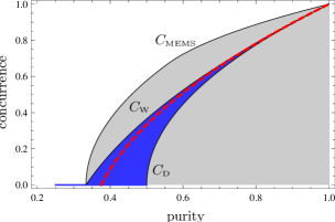
Figure 1: (Color online) The CP diagram. The light gray area shows the region of all physical states of two qubits, bounded by the maximally entangled mixed states ($C_{\mbox{\tiny MEMS}}$). The possible $C(P)$ relations for a Bell state subject to single-sided unital dynamics or, equivalently, of all doubly chaotic states, is highlighted in blue (dark gray). This region is bounded by the curves valid for Werner states $C_{\mbox{\tiny W}}$ and for Bell states under single-sided phase damping $C_{\mbox{\tiny D}}$, respectively. The diagram also reveals the maxium $C(P)$ relation of doubly chaotic states with Bell rank $3$, $C_{3}(P)$ (dashed line).

Aside from the border of all physical states given by $C_{\mbox{\tiny MEMS}}$, the diagram reveals the accessible region (blue) for initial Bell states under single-sided unital channels $\mathcal{E}\otimes\mathds{1}$, that is, unital channels acting on either one of the subsystems, only. This accessible region found is bounded by the curves $C_{\mbox{\tiny W}}$ and $C_{\mbox{\tiny D}}$ that are realized for single-sided depolarization and single-sided phase damping, respectively. The former is also valid for the so-called Werner states Werner1989 , $\varrho_{W}=p\left|\psi_{S}\right\rangle\left\langle\psi_{S}\right|+(1-p)\mathds{1}/4$, a convex mixture of the pure and maximally entangled singlet state $\left|\psi_{S}\right\rangle=(\left|01\right\rangle-\left|10\right\rangle)/\sqrt{2}$ and the maximally disordered two-qubit state $\mathds{1}/4$.

These borders will also play an important role in our findings. We start by rederiving the results found in Ref. Ziman2005 in an alternative way. It is known that in case of single-qubit dynamics there is a one-to-one correspondence between unital channels and channels that are RU LandauStreater . By applying the quantum channel $\mathcal{E}$ to one part of a maximally entangled bipartite state, the so-called Jamiolkowski isomorphism ZyczkowskiBook introduces a duality between quantum channels defined on a Hilbert space $\mathcal{H}$ and quantum states living on a Hilbert space $\mathcal{H}\otimes\mathcal{H}$ of squared dimension. It follows straight away that the Jamiolkowski state of a RU channel is doubly chaotic LandauStreater , that is, the state has maximally disordered subsystems: $\mbox{tr}_{1}\varrho=\mbox{tr}_{2}\varrho=\mathds{1}/d$ (here, $\mbox{tr}_{i}$, $i=1,2$, refers to a partial trace over the first and second subsystems, respectively, while $d=\dim\mathcal{H}$). In this vein, any single-qubit RU channel may be identified with a doubly chaotic two-qubit state. Any such state may in turn be obtained by applying a local unitary transformation $U\otimes V$ to a Bell-diagonal state Horodecki1996 , that is, a state diagonal in the basis of Bell states $\left|\psi^{\tiny\mbox{B}}_{i}\right\rangle$:

$$\varrho=U\otimes V\left(\sum_{i=1}^{m}p_{i}|\psi^{\tiny\mbox{B}}_{i}\rangle\langle\psi^{\tiny\mbox{B}}_{i}|\right)U^{\dagger}\otimes V^{\dagger}$$

with $\sum_{i}p_{i}=1$.

For such a state the accessible area in the CP diagram may be determined easily (see Appendix C). As a general lower bound we find the relation $C(P)=\sqrt{2P-1}=C_{\mbox{\tiny D}}$, whereas the upper bound depends on the Kraus rank $k$ of the corresponding qubit channel $\mathcal{E}$, that is, on the minimum number of Kraus operators needed in (1). For $k=2$ we have

$$C_{2}(P) = C_{\mbox{\tiny D}}=\sqrt{2P-1},\quad P\geq\frac{1}{2},$$ (7)

again identical to the lower bound in the CP diagram, whereas for $k=4$ we have

$$C_{4}(P) = C_{\mbox{\tiny W}}=\frac{1}{2}\left(\sqrt{12\,P-3}-1\right),\quad P\geq\frac{1}{3},$$ (8)

reproducing the upper bound. In addition, we get the relation

$$C_{3}(P) = \frac{1}{3}\left(\sqrt{24\,P-8}-1\right),\quad P\geq\frac{3}{8},$$ (9)

giving an upper bound of the allowed area for single-sided RU channels of Kraus rank 3 (see Fig. 1, dashed line).

Thus, we arrive at the same results that were obtained by applying single-sided unital channels to a pure and maximally entangled two-qubit state Ziman2005 . We find that the accessible region in the CP plane depends on the Kraus rank of the RU channel. It is then quite obvious that the lower and upper border are given by single-sided phase damping (Kraus rank 2) and depolarizing (Kraus rank 4), respectively. The various bounds in the CP diagram may be attributed to a characteristic trait of doubly chaotic states. This is also true for the behavior discovered in Torres2009 , where for an initial Bell state of two noninteracting qubits with symmetric coupling to a cavity with photon number $n\rightarrow\infty$ a convergence to $C_{3}(P)$ was found. In this limit, the Bell state is simply mapped to a doubly chaotic state with Bell rank 3, hence explaining the asymptotic behavior.

For random local unitary (RLU) channels, that is, channels of the form $\mathcal{E}(\varrho)=\sum_{r,s}p_{rs}(U_{r}\otimes V_{s})\varrho(U_{r}^{\dagger}\otimes V_{s}^{\dagger})$, with $\sum_{r,s}p_{rs}=1$ and unitary $U_{r},V_{s}$, it is easy to see that a Bell state is mapped to a doubly chaotic state. Comparison with Eq. (II) shows that the action of the noise channel $\tilde{D}$ is exactly of this RLU nature. Therefore, it is by no means surprising that the bounds play a role in our findings. Note, however, that our studies cover not only the case of maximally entangled initial states, but of pure initial states in general. Based on our derivation it also follows immediately that the accessible region for bilocal unital dynamics $\mathcal{E}_{1}\otimes\mathcal{E}_{2}$—a question raised in Ref. Ziman2005 —is in fact identical to the area obtained for single-sided unital channels.

IV Separable initial state

In Sec. II we discussed the possible separation of the RU phase-damping channel, making it possible to separately calculate the evolution of purity and entanglement. The general formula for purity of the final state was already given, Eq. (II), whereas in order to study entanglement, we need to make further assumptions about the initial state. In this first section we take the initial state to be separable. Due to the commutativity of the noise channel $\tilde{D}$ and the unitary part $U_{\mu}$, we can start out by bringing a pure separable state $\varrho:=\left|\psi_{0}\right\rangle\left\langle\psi_{0}\right|:=\left|\phi_{1}\right\rangle\left\langle\phi_{1}\right|\otimes\left|\phi_{2}\right\rangle\left\langle\phi_{2}\right|$ into the mixture $\tilde{D}\star\varrho$, prior to applying $U_{\mu}$. For the final state $\varrho^{\prime}$ we will then calculate the concurrence $C$. For generic single-qubit states we can let

$$\left|\phi_{i}\right\rangle:=\begin{pmatrix}\alpha_{i}\\ \beta_{i}\end{pmatrix},\;i=1,2,$$

with $\alpha_{i},\beta_{i}\in\mathds{C},|\alpha_{i}|^{2}+|\beta_{i}|^{2}=1$. The calculation of the concurrence of $\varrho^{\prime}$ involves the determination of the eigenvalues of the positive, non-Hermitian matrix $R=\varrho^{\prime}(\sigma_{y}\otimes\sigma_{y})\varrho^{\prime*}(\sigma_{y}\otimes\sigma_{y})$. We find (see Appendix D)

$$C(\varrho^{\prime}) = g(\left|\psi_{0}\right\rangle)\cdot f(\mathcal{E}),$$ (10)

where

$$g(\left|\psi_{0}\right\rangle) = 4|\alpha_{1}||\beta_{1}||\alpha_{2}||\beta_{2}|=\sqrt{\mbox{var}(\sigma_{z}^{A})}\sqrt{\mbox{var}(\sigma_{z}^{B})},$$

$$f(\mathcal{E}) = \mbox{max}\Big{\{}0,(p_{1}-p_{2})\sin\mu_{3}$$

$$\quad-\sqrt{(p_{3}+p_{4})^{2}\sin^{2}\mu_{3}+4p_{3}p_{4}\cos^{2}\mu_{3}}\Big{\}}.$$

With $\mbox{var}(\sigma_{z}^{i})=1-\langle\sigma_{z}^{i}\rangle^{2}$ we denote the variances of $\sigma_{z}^{i}$ ($i=A,B$), which can be taken with respect to the initial state $\left|\psi_{0}\right\rangle$. The mean value $\mu_{3}=\left\langle\!\left\langle\Omega_{3}\right\rangle\!\right\rangle$, as well as the probabilities $p_{i}$, were introduced in Sec. II and reflect mean value and variance of the fluctuating fields (see also App. B).

The concurrence thus allows for an evolution equation factorizing into two functionals $f$ and $g$ that depend on the phase-damping channel $\mathcal{E}$ and the initial state of the qubits $\left|\psi_{0}\right\rangle$, respectively. The evolution equation accounts for the gain in entanglement due to the unitary map $U_{\mu}$ through the function $f$, while $g$ simply gives a scaling factor for the amount of entanglement a certain initial state may achieve.

When trying to detect the accessible area within the CP diagram we need to know the maximum of the concurrence with respect to the entangling part of the channel. This maximum is given for $\sin\mu_{3}=1$ or, equivalently, $\mu_{3}\in\{(2k+1)\frac{\pi}{2}\;|\;k\in\mathds{Z}\}$, which leads to the simple equation

$$C_{\mbox{\tiny Max}} = \!\mbox{max}\Big{\{}0,g(\left|\psi_{0}\right\rangle)\;(p_{1}-p_{2}-p_{3}-p_{4})\Big{\}}$$

$$= \!\mbox{max}\Big{\{}0,g(\left|\psi_{0}\right\rangle)$$

$$\quad\times\frac{1}{2}\Big{[}e^{-\left(\varsigma_{1}^{2}+\varsigma_{2}^{2}\right)}+e^{-\left(\varsigma_{1}^{2}+\varsigma_{3}^{2}\right)}+e^{-\left(\varsigma_{2}^{2}+\varsigma_{3}^{2}\right)}-1\Big{]}\!\Big{\}}.$$

IV.1 Pure two-qubit phase damping

We want to discuss the results obtained so far in a setting where we admit only pure two-qubit phase damping. By this we mean the situation where the phase damping is caused by a fluctuation in the part of the Hamiltonian describing the coupling of the two qubits only. Note that this setting is also of relevance in the realization of a phase gate in recent ion-trap experiments Monz2009 . The Hamiltonian then consists of the single term $H(t)=\omega_{3}(t)\sigma_{z}^{A}\otimes\sigma_{z}^{B}$. Recall the definition of the variances $2\varsigma_{k}^{2}=\left\langle\!\left\langle\Omega_{k}^{2}\right\rangle\!\right\rangle-\left\langle\!\left\langle\Omega_{k}\right\rangle\!\right\rangle^{2}$ (cf. Sec. II). We may therefore let the variances $\varsigma_{1}=\varsigma_{2}=0$, and Eq. (IV) simplifies to

$$C_{\mbox{\tiny Max}}(\varrho^{\prime})=e^{-\varsigma_{3}^{2}}\cdot g(\left|\psi_{0}\right\rangle),$$ (12)

whereas the purity simplifies to

$$P(\varrho^{\prime}) = \frac{1}{2}(1+e^{-2\varsigma_{3}^{2}})+$$

$$\quad\frac{1}{2}(1-e^{-2\varsigma_{3}^{2}})\cdot|\langle\sigma_{z}^{A}\rangle|^{2}\cdot|\langle\sigma_{z}^{B}\rangle|^{2}.$$

The simple form of both the maximal concurrence and the purity enables us to give the former as a function of the latter:

$$C_{\mbox{\tiny Max}}(P) = \sqrt{\frac{\big{(}1-\langle\sigma_{z}^{A}\rangle^{2}\big{)}\,\big{(}1-\langle\sigma_{z}^{B}\rangle^{2}\big{)}}{1-\langle\sigma_{z}^{A}\rangle^{2}\langle\sigma_{z}^{B}\rangle^{2}}}\times$$ (14)

$$\quad\sqrt{2P-1-\langle\sigma_{z}^{A}\rangle^{2}\langle\sigma_{z}^{B}\rangle^{2}}.$$

Note that for $\langle\sigma_{z}^{A}\rangle=\langle\sigma_{z}^{B}\rangle=0$ we get $C_{\mbox{\tiny Max}}(P)=\sqrt{2P-1}$, which is exactly the equation obtained for the lower bound $C_{\mbox{\tiny D}}$ shown in Fig. 1.

In Fig. 2 we show the CP diagram where we highlight the excluded area. In order to show exemplary dynamics in the diagram we let both mean and variances of the stochastic processes in Eq. (3) depend quadratically on some “time parameter” $t$. This introduces a one-parameter class of channels $\mathcal{E}_{t}$ mimicking continuous dynamics. A possible evolution is shown as blue line.

Equation (14) relating maximal concurrence and purity allows for a representation of the accessible region under pure two-qubit phase damping (for an initially separable state). For this we define $Z$ as the expectation value of the number of excited states, that is, $Z:=1+\frac{\langle\sigma_{z}^{A}\rangle+\langle\sigma_{z}^{B}\rangle}{2}$. When maximizing the function $C_{\mbox{\tiny Max}}(P)$ for fixed $P$ and $Z$, we get the requirement $\langle\sigma_{z}^{A}\rangle=\langle\sigma_{z}^{B}\rangle=:\langle\sigma_{z}\rangle$. Inserted in (14), this leads to

$$C_{\mbox{\tiny Max}}(P,\langle\sigma_{z}\rangle)=\sqrt{\frac{1-\langle\sigma_{z}\rangle^{2}}{1+\langle\sigma_{z}\rangle^{2}}(2P-1-\langle\sigma_{z}\rangle^{4})}.$$ (15)

This relation can now be visualized in the concurrence-purity-$\langle\sigma_{z}\rangle$ space [cf. Fig. 2 (b)]. This representation was also used in McHugh2006 , where the physically allowed region of a two-qubit system with respect to concurrence, purity, and energy was studied.

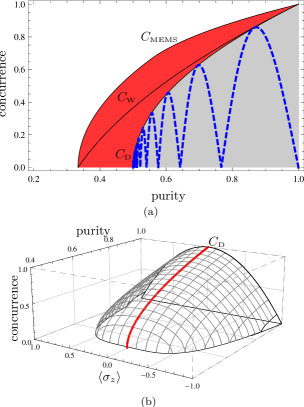
Figure 2: (Color online) (a) For a pure separable initial state subject to pure two-qubit phase damping, the maximally achievable concurrence is bounded from above by $C_{\mbox{\tiny D}}$. The corresponding forbidden area is highlighted in red (dark gray). The blue (dashed) line represents the evolution under a one-parameter class of phase-damping channels (see text for details). (b) The accessible value of concurrence depends on expectation value $\langle\sigma_{z}^{(i)}\rangle$ evaluated for either one of the qubits $i=A,B$. Only for $\langle\sigma_{z}^{A}\rangle=\langle\sigma_{z}^{B}\rangle=0$ may the relation $C_{\mbox{\tiny D}}$ (red, thick line) be obtained.

IV.2 General uncorrelated phase damping

Next we want to consider the general case of uncorrelated phase damping. Remember that by uncorrelated we mean a diagonal covariance matrix $\Sigma$. Here, we use the full dynamics, that is, the part of the Hamiltonian describing pure two-qubit dephasing as well as the parts acting locally on both qubits.

As in the preceding section, the concurrence attains its maximum for $\langle\sigma_{z}^{A}\rangle=\langle\sigma_{z}^{B}\rangle=0$, leading to the identities

$$C = \frac{1}{2}\left[e^{-\left(\varsigma_{1}^{2}+\varsigma_{2}^{2}\right)}+e^{-\left(\varsigma_{1}^{2}+\varsigma_{3}^{2}\right)}+e^{-\left(\varsigma_{2}^{2}+\varsigma_{3}^{2}\right)}-1\right]$$ (16)

$$P = \frac{1}{4}\left[e^{-2\left(\varsigma_{1}^{2}+\varsigma_{2}^{2}\right)}+e^{-2\left(\varsigma_{1}^{2}+\varsigma_{3}^{2}\right)}+e^{-2\left(\varsigma_{2}^{2}+\varsigma_{3}^{2}\right)}+1\right].$$ (17)

Note that for identical variances $\varsigma_{1}=\varsigma_{2}=\varsigma_{3}=:\varsigma$, this implies $C=\frac{1}{2}\big{(}3e^{-2\varsigma^{2}}-1\big{)}$ and $P=\frac{1}{4}\big{(}3e^{-4\varsigma^{2}}+1\big{)}$, which is easily transformed into the relation

$$C(P)=\frac{1}{2}\left(\sqrt{12\,P-3}-1\right),\quad P\geq\frac{1}{3},$$ (18)

which coincides with the relation obtained for the Werner states, $C_{\mbox{\tiny W}}$.

Furthermore, from Eqs. (16) and (17) we conclude that $C^{2}+C+1\leq 3P$, so that the case of all variances being equal already yields the maximal relation of concurrence as a function of purity. We conclude that $C_{\mbox{\tiny Max}}(P)=(\sqrt{12P-3}-1)/2$ in case of uncorrelated phase damping. For pure, separable states subject to RU phase damping, we can therefore identify a forbidden area in the CP plane, the border of which is given by the Werner states $C_{\mbox{\tiny W}}$. In Fig. 3 (a) we highlight the excluded area for general, uncorrelated phase damping.

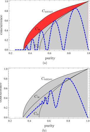
Figure 3: (Color online) (a) In case of general uncorrelated phase damping, the maximally achievable concurrence is identical to the value given by the Werner states, $C_{\mbox{\tiny W}}$. As before, the forbidden area is highlighted in red (dark gray). The role of correlations may be observed in (b), where both bounds are violated. In both diagrams, an exemplary evolution under a one-parameter class of phase-damping channels is shown (dashed blue lines).

Note that these results are only true for uncorrelated phase damping. In Fig. 3 (b) we show an example of correlated phase damping, that is, with nondiagonal covariance matrix $\Sigma$ (see Sec. II). This accentuates the fact that the borders in the CP diagram are valid only in the uncorrelated case. We ascribe this violation of the bounds in case of correlated phase damping to the fact that the irreversible part of the channel $\tilde{D}$ is in general no longer RLU (see Sec. III).

V General Pure Initial State

In this section we will analyze the evolution of a general pure initial state under phase damping, that is, we drop the restriction of separability for the initial state. For our purposes, that is, for entanglement and purity evolution under phase damping, the most general (pure) intial state reads

$$\left|\psi_{0}\right\rangle = \big{(}e^{-\frac{i}{2}\theta_{1}\sigma_{x}}\otimes e^{-\frac{i}{2}\theta_{2}\sigma_{x}}\big{)}\times$$

$$\quad\quad\left(\sqrt{a}\left|00\right\rangle+e^{-i\chi}\sqrt{1-a}\left|11\right\rangle\right),$$

leaving only four parameters $(a,\chi,\theta_{1},\theta_{2})$ to fully characterize the initial state of the two-qubit system (see Appendix E).

While Eq. (II), giving the purity of the final state, is still valid, we need to estimate the decay of the initial concurrence when the state is subject to the mixing part of the phase damping channel, $\tilde{D}$. In close analogy to the method described in Appendix D, we are again able to estimate the concurrence analytically:

$$C(\varrho^{\prime}) = \mbox{Max}\Big{\{}0,$$

$$\!\!\!\!\!\!\!\sqrt{(p_{1}^{2}+p_{2}^{2})|s|^{2}+2p_{1}p_{2}|r|^{2}-2p_{1}p_{2}|s^{2}-r^{2}|}-$$

$$\!\!\!\!\!\!\!\sqrt{(p_{3}^{2}+p_{4}^{2})|s|^{2}+2p_{3}p_{4}|r|^{2}+2p_{3}p_{4}|s^{2}-r^{2}|}\Big{\}},$$

where we have defined $s:=\left\langle\psi_{0}\right|\Sigma_{y}\left|\psi_{0}^{*}\right\rangle$ and $r:=\left\langle\psi_{0}\right|\Sigma_{z}\Sigma_{y}\left|\psi_{0}^{*}\right\rangle$. Here we have also used the abbreviations $\Sigma_{i}:=\sigma_{i}\otimes\sigma_{i}$ ($i=x,y,z$).

Together with the purity (II) we can now examine the possible $C(P)$ combinations in more detail. In order to get illustrative results, we again have to put some further constraints on the dynamics.

V.1 Single-sided phase damping

For a single-sided phase-damping channel, that is, acting on either one of the qubits, we can generalize the results obtained for maximally entangled states in Ref. Ziman2005 to the case of pure initial states with arbitrary entanglement. Note that for this scenario the channel is simply given by $\varrho^{\prime}=(1-q)\varrho+q(\sigma_{z}^{A}\otimes\mathds{1})\varrho(\sigma_{z}^{A}\otimes\mathds{1})$.

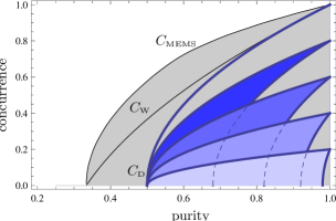
Figure 4: (Color online) Accessible region for a single-sided phase damping channel for states of varying initial entanglement $C_{\scriptstyle 0}=0.2\;(0.4,\;0.6,\;0.8,\;1)$. For $C_{\scriptstyle 0}=1$, the lower and upper bounds are equal, given by the known curve $C_{\mbox{\tiny D}}$.

For single-sided phase damping it is easy to arrive at the evolution equation of entanglement, which is given by

$$C(\varrho^{\prime})=f(\mathcal{E})\cdot C_{0},$$

where $f(\mathcal{E})=1-2q$. The state-dependent behavior within the CP diagram thus stems from the evolution of purity, which is given by

$$P(\varrho^{\prime})=1-2q(1-q)\left[1-|\langle\sigma_{z}^{A}\rangle|^{2}\right],$$

where $|\langle\sigma_{z}^{A}\rangle|^{2}=\cos^{2}\theta_{1}(2a-1)^{2}$.

We find that the $C(P)$ relation for given initial entanglement now only depends on the angle $\theta_{1}$ . The extremal cases may be identified as

$$C(P)=\left\{\begin{array}[]{cc}\sqrt{C_{0}^{2}(2P-1)}&\mbox{if }\cos^{2}\theta_{1}=0\\ \sqrt{C_{0}^{2}+2(P-1)}&\mbox{if }\cos^{2}\theta_{1}=1\end{array}\right.$$

where $C_{0}$ denotes the concurrence of the initial state $\left|\psi_{0}\right\rangle$. For all other cases ($0\leq\cos^{2}\theta_{1}\leq 1$), one can see that the relation $C(P)$ is bounded by these two curves. For maximally entangled initial states the two functions coincide, again giving the by-now well-known relation $C(P)=\sqrt{2P-1}=C_{\mbox{\tiny D}}$ Ziman2005 . For nonextremal initial entanglement $0<C_{0}<1$, however, the two curves part, bounding the accessible region from above and below. For states of arbitrary initial entanglement subject to single-sided phase damping we conclude that there exists a maximal value of purity, $P_{<}=1-C_{0}^{2}/2$, above which all states are still entangled. Again, the results are easily illustrated using the CP diagram (see Fig. 4).

V.2 Pure two-qubit phase damping

In case of pure two-qubit phase damping, the noise channel is of the simple form $\varrho^{\prime}=(1-q)\varrho+q(\sigma_{z}^{A}\otimes\sigma_{z}^{B})\varrho(\sigma_{z}^{A}\otimes\sigma_{z}^{B})$. Again we are able to give the evolution equation of entanglement,

$$C^{2}(\varrho^{\prime}) = C_{0}^{2}-2q(1-q)\left[|r|^{2}-|s|^{2}-|r^{2}-s^{2}|\right]$$ (20)

$$=: C_{0}^{2}-f(\mathcal{E})\cdot g(\left|\psi_{0}\right\rangle),$$

where now $f(\mathcal{E})=2q(1-q)$ and $g(\left|\psi_{0}\right\rangle)=|r|^{2}-|s|^{2}-|r^{2}-s^{2}|$. Entanglement depends on the initial state of the two qubits through the functional $g$. Note that here the evolution equation no longer follows the factorization law, as in the case of single-sided channels. Yet the evolution is fully determined through the functionals $f$ and $g$. The purity equates to

$$P(\varrho^{\prime})=1-2q(1-q)\left[1-|\langle\sigma_{z}^{A}\otimes\sigma_{z}^{B}\rangle|^{2}\right]$$ (21)

with $|\langle\sigma_{z}^{A}\otimes\sigma_{z}^{B}\rangle|^{2}=\big{[}\cos\theta_{1}\cos\theta_{2}-\sin\theta_{1}\sin\theta_{2}\cdot\cos\chi\cdot 2\sqrt{a(1-a)}\big{]}^{2}$.

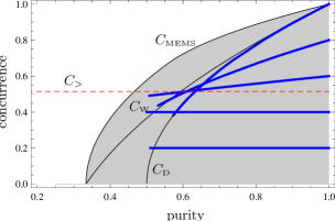
Figure 5: (Color online) For pure two-qubit phase damping we can identify states with robust entanglement. The plot is obtained for an initial state parameterized by $\chi=0,\,\theta_{1}=3\pi/16,\,\theta_{2}=\pi/8$ (see text), leading to robust entanglement for $C_{0}\leq C_{>}\approx 0.5142$ (dashed red line). The blue (thick) lines show exemplary evolution of pure states with initial concurrence $C_{0}=1.0\;(0.8,\;0.6,\;0.4,\;0.2)$.

Eq. (20) highlights the possibility of robust entanglement under pure two-qubit phase damping. It is easy to see that for $g(\left|\psi_{0}\right\rangle)=0$ concurrence remains constant, whereas purity [Eq. (21)] may, in general, still decline. We find that this is the case for states with $\chi\in\{k\pi|k\in\mathds{Z}\}$, only. The square of the concurrence then becomes

$$C^{2}(\varrho^{\prime})=\left\{\begin{array}[]{l@{\quad}l}s^{2}-4q(1-q)[C_{0}^{2}-r^{2}]&\mbox{if }s^{2}>r^{2}\\ s^{2}&\mbox{if }s^{2}\leq r^{2}.\end{array}\right.$$

The necessary condition for robust entanglement under pure two-qubit phase damping is thus given by $s^{2}\leq r^{2}$ and $\chi=k\pi$. To be specific, the necessary conditions for $\chi=k2\pi$ [$\chi=(2k+1)\pi$] are given by

$$s^{2}\leq r^{2}$$

$$\Leftrightarrow$$

$$C_{0}\leq C_{>}:=\mbox{max}\left\{[-]\frac{\sin\theta_{1}\sin\theta_{2}}{\cos\theta_{1}\cos\theta_{2}+1},[-]\frac{\sin\theta_{1}\sin\theta_{2}}{\cos\theta_{1}\cos\theta_{2}-1}\right\},$$

hereby defining the upper bound $C_{>}$, such that states with initial concurrence $C_{0}<C_{>}$ exhibit robust entanglement. Note that for $\cos\theta_{1}\cos\theta_{2}=\pm 1$, $s^{2}=r^{2}$ and, thus, constant concurrence $C$ follows immediately. In Fig. 5 we show an example of robust entanglement. It can be clearly observed that for initial concurrence smaller than $C_{>}$ and despite the loss of purity, the entanglement is persistent. Beyond the observation of robust entanglement we also see that, while the map of the maximally entangled state follows the line $C_{\mbox{\tiny D}}$, as would be predicted (the Kraus rank of pure two-qubit phase damping is 2, see Sec. III), for states with initial concurrence $C_{0}<1$, the restricted area no longer plays a role.

VI Conclusions

We have studied a two-qubit quantum system subject to phase damping caused by fluctuating fields. Irrespective of possible correlations between the individual constituents of the introduced stochastic Hamiltonian, the quantum channel was shown to allow a separation into two parts, representing reversible and irreversible parts of the dynamics, respectively. The separation enabled us to estimate the evolution of the system’s entanglement, as well as purity, analytically. When combined, the results allow us to identify exclusive regions within the concurrence-purity plane, suggesting a connection between RLU dynamics on a Bell state and phase-damping processes on a separable initial state. These forbidden places, however, do not play a role in the evolution of pure states of arbitrary initial entanglement $0<C_{0}<1$.

Our approach enables us to generalize results obtained in Ref. Ziman2005 , where the action of single-sided unital channels on Bell states was studied. Here we are able to analyze the effect of single-qubit phase damping on pure two-qubit states of arbitrary initial entanglement. For a certain class of phase damping we have identified necessary conditions leading to a robustness of the entanglement present in the two-qubit system. This robustness is closely related to the entanglement of the initial state; more precisely, depending on the initial state, we can give an upper bound $C_{>}$ such that for all states with concurrence $C_{0}<C_{>}$ the entanglement is robust. The crucial conclusion to be drawn from these findings is that in order to preserve entanglement, sometimes less is more.

Appendix A

In Sec. II we present the decomposition (II) of the phase-damping channel into unitary part and noise channel. In order to see this, recall the definition of the RU channel

$$\varrho\mapsto\varrho^{\prime}=\left\langle\!\left\langle U(t)\varrho U^{\dagger}(t)\right\rangle\!\right\rangle.$$

The unitary map is given by $U(t)=e^{-i\int_{0}^{t}d\tau H(\tau)}$, where in our model

$$H(t)=\omega_{1}(t)\sigma_{z}^{A}\otimes\mathds{1}+\omega_{2}(t)\mathds{1}\otimes\sigma_{z}^{B}+\omega_{3}(t)\sigma_{z}^{A}\otimes\sigma_{z}^{B}.$$

A simple calculation gives the diagonal map

$$\varrho^{\prime}_{mn} = \left\langle\!\left\langle e^{i\sum_{k=1}^{3}c_{k}^{mn}\Omega_{k}}\right\rangle\!\right\rangle\varrho_{mn}$$ (23)

$$= e^{i\sum_{k=1}^{3}c_{k}^{mn}\left\langle\!\left\langle\Omega_{k}\right\rangle\!\right\rangle}\left\langle\!\left\langle e^{i\sum_{k=1}^{3}c_{k}^{mn}\left(\Omega_{k}-\left\langle\!\left\langle\Omega_{k}\right\rangle\!\right\rangle\right)}\right\rangle\!\right\rangle\varrho_{mn}$$

$$=: D^{\mu}_{mn}\tilde{D}_{mn}\varrho_{mn},$$

where we have used the compact notation $c_{k}^{mn}:=(\vec{e}_{m}-\vec{e}_{n})_{k}$ with vectors $\vec{e}_{1}=(0,0,0),\vec{e}_{2}=(0,1,1),\vec{e}_{3}=(1,0,1),\vec{e}_{4}=(1,1,0)$, as well as the abbreviations $D^{\mu}_{mn}=e^{i\sum_{k=1}^{3}c_{k}^{mn}\left\langle\!\left\langle\Omega_{k}\right\rangle\!\right\rangle}$ and $\tilde{D}_{mn}=\left\langle\!\left\langle e^{i\sum_{k=1}^{3}c_{k}^{mn}\left(\Omega_{k}-\left\langle\!\left\langle\Omega_{k}\right\rangle\!\right\rangle\right)}\right\rangle\!\right\rangle$. The diagonal map $D^{\mu}_{mn}$ may be rewritten in terms of a diagonal unitary transformation $U_{\mu}=e^{-iH_{\mu}t}$ such that $D^{\mu}_{mn}=(U_{\mu})_{mm}(U_{\mu})^{*}_{nn}$, where the Hamiltonian $H_{\mu}$ is determined by the mean values $\left\langle\!\left\langle\Omega_{k}\right\rangle\!\right\rangle=:\mu_{k}$ :

$$H_{\mu}:=\mu_{1}\sigma_{z}^{A}\otimes\mathds{1}+\mu_{2}\mathds{1}\otimes\sigma_{z}^{B}+\mu_{3}\sigma_{z}^{A}\otimes\sigma_{z}^{B}.$$

Commutativity of unitary part $U_{\mu}$ and noise channel $\tilde{D}$ is then a direct consequence of the diagonality (23) of the two maps. Formally, we may thus write

$$\varrho^{\prime} = U_{\mu}(\tilde{D}\star\varrho)U_{\mu}^{\dagger}$$

$$= D^{\mu}\star(\tilde{D}\star\varrho)$$

$$= \tilde{D}\star(D^{\mu}\star\varrho)$$

$$= \tilde{D}\star\left(U_{\mu}\varrho U_{\mu}^{\dagger}\right).$$

Appendix B

The probabilities used in Sec. II in terms of the variances $2\varsigma_{k}^{2}=\left\langle\!\left\langle\Omega_{k}^{2}\right\rangle\!\right\rangle-\left\langle\!\left\langle\Omega_{k}\right\rangle\!\right\rangle^{2}$ are given as follows:

$$p_{1} = \frac{1}{8}\left\{\left(1+e^{-\varsigma_{1}^{2}}\right)\left(1+e^{-\varsigma_{2}^{2}}\right)\left(1+e^{-\varsigma_{3}^{2}}\right)+\left(1-e^{-\varsigma_{1}^{2}}\right)\left(1-e^{-\varsigma_{2}^{2}}\right)\left(1-e^{-\varsigma_{3}^{2}}\right)\right\}$$

$$p_{2} = \frac{1}{8}\left\{\left(1+e^{-\varsigma_{1}^{2}}\right)\left(1+e^{-\varsigma_{2}^{2}}\right)\left(1-e^{-\varsigma_{3}^{2}}\right)+\left(1-e^{-\varsigma_{1}^{2}}\right)\left(1-e^{-\varsigma_{2}^{2}}\right)\left(1+e^{-\varsigma_{3}^{2}}\right)\right\}$$

$$p_{3} = \frac{1}{8}\left\{\left(1+e^{-\varsigma_{1}^{2}}\right)\left(1-e^{-\varsigma_{2}^{2}}\right)\left(1-e^{-\varsigma_{3}^{2}}\right)+\left(1-e^{-\varsigma_{1}^{2}}\right)\left(1+e^{-\varsigma_{2}^{2}}\right)\left(1+e^{-\varsigma_{3}^{2}}\right)\right\}$$

$$p_{4} = \frac{1}{8}\left\{\left(1+e^{-\varsigma_{1}^{2}}\right)\left(1-e^{-\varsigma_{2}^{2}}\right)\left(1+e^{-\varsigma_{3}^{2}}\right)+\left(1-e^{-\varsigma_{1}^{2}}\right)\left(1+e^{-\varsigma_{2}^{2}}\right)\left(1-e^{-\varsigma_{3}^{2}}\right)\right\}.$$

Appendix C

In Sec. III we argue that any unital single-qubit channel may be identified with a doubly chaotic two-qubit state. A given doubly chaotic state of two qubits may in turn be obtained by applying a local unitary transformation $U\otimes V$ to a Bell-diagonal state Horodecki1996 :

$$\varrho=U\otimes V\left(\sum_{i=1}^{m}p_{i}|\psi^{\tiny\mbox{B}}_{i}\rangle\langle\psi^{\tiny\mbox{B}}_{i}|\right)U^{\dagger}\otimes V^{\dagger}$$

with probabilities $p_{i}$, $\{\left|\Psi_{i}^{\tiny\mbox{B}}\right\rangle\}_{i=1,...,4}$ denotes the basis of Bell states. By rearrangement of the Bell basis let $p_{1}\geq p_{2}\geq p_{3}\geq p_{4}$, so that $m$ denotes the Bell rank of $\varrho$, that is, the minimum number of Bell states needed to represent the state $\varrho$. Note that the Bell rank is equal to the so-called Kraus rank of the channel, which gives the minimum number of terms in the Kraus representation (1). Using the Bell-diagonal representation, both concurrence and purity are of a very simple form:

$$C(\varrho)=\max\{0,2p_{1}-1\},\quad\quad P(\varrho)=\sum_{i=1}^{m}p_{i}^{2}.$$ (24)

The maximum relation $C(P)$ now depends on the Bell rank $m$. It may be obtained by minimizing the purity for given concurrence. Let $p_{1}=:1-q$, then from Eqs. (24) we can conclude that the purity is minimal if the remaining weights $p_{i}$ with $i>1$ are equal, $p_{i}=q/(m-1)$. We thus obtain

$$C(\varrho) = \max\{0,1-2q\},$$

$$P(\varrho) \geq 1-2q\left(1-q\frac{m}{m-1}\right),$$

and we can immediately give an upper bound for the concurrence as a function of purity: $C(P)\leq 2\frac{m-1}{m}\sqrt{\frac{mP-1}{m-1}}-\frac{m-2}{m}=:C_{m}(P)$. Inserting the nontrivial Bell ranks $m=2,3,4$, we get the upper bounds of the accessible $C(P)$ relations for single-sided RU channels with corresponding Kraus ranks. Moreover, we see that for arbitrary Kraus rank $k$, $C(P)$ is bounded from below by $C_{2}(P)$.

Appendix D

The calculation of the concurrence involves the determination of the eigenvalues of the positive, non-Hermitian matrix

$$R = \varrho^{\prime}\;\tilde{\varrho}^{\prime}$$

$$= 4\alpha_{1}^{*}\beta_{1}^{*}\alpha_{2}^{*}\beta_{2}^{*}\times$$

$$\Big{[}\;e^{-i\boldsymbol{\tilde{\varphi}}}\left|\psi_{0}\right\rangle\Big{\{}-ip_{1}^{2}\sin\mu_{3}\left\langle\psi_{0}^{*}\right|\Sigma_{y}e^{-i\boldsymbol{\tilde{\varphi}}}-p_{1}p_{2}\cos\mu_{3}\left\langle\psi_{0}^{*}\right|\Sigma_{y}\Sigma_{z}e^{-i\boldsymbol{\tilde{\varphi}}}\Big{\}}$$

$$\;+e^{-i\boldsymbol{\tilde{\varphi}}}\Sigma_{z}\left|\psi_{0}\right\rangle\Big{\{}-p_{1}p_{2}\cos\mu_{3}\left\langle\psi_{0}^{*}\right|\Sigma_{y}e^{-i\boldsymbol{\tilde{\varphi}}}-ip_{2}^{2}\sin\mu_{3}\left\langle\psi_{0}^{*}\right|\Sigma_{y}\Sigma_{z}e^{-i\boldsymbol{\tilde{\varphi}}}\Big{\}}$$

$$\;+e^{-i\boldsymbol{\tilde{\varphi}}}\sigma_{z}\otimes\mathds{1}\left|\psi_{0}\right\rangle\Big{\{}ip_{3}^{2}\sin\mu_{3}\left\langle\psi_{0}^{*}\right|\Sigma_{y}(\sigma_{z}\otimes\mathds{1})e^{-i\boldsymbol{\tilde{\varphi}}}+p_{3}p_{4}\cos\mu_{3}\left\langle\psi_{0}^{*}\right|\Sigma_{y}(\mathds{1}\otimes\sigma_{z})e^{-i\boldsymbol{\tilde{\varphi}}}\Big{\}}$$

$$\;+e^{-i\boldsymbol{\tilde{\varphi}}}\mathds{1}\otimes\sigma_{z}\left|\psi_{0}\right\rangle\Big{\{}p_{3}p_{4}\cos\mu_{3}\left\langle\psi_{0}^{*}\right|\Sigma_{y}(\sigma_{z}\otimes\mathds{1})e^{-i\boldsymbol{\tilde{\varphi}}}+ip_{4}^{2}\sin\mu_{3}\left\langle\psi_{0}^{*}\right|\Sigma_{y}(\mathds{1}\otimes\sigma_{z})e^{-i\boldsymbol{\tilde{\varphi}}}\Big{\}}\Big{]},$$

where we have defined $\Sigma_{i}:=\sigma_{i}\otimes\sigma_{i}$ ($i=x,y,z$) and $\boldsymbol{\tilde{\varphi}}:=\mu_{3}\Sigma_{z}/2$.

We find the existence of two $R$-invariant linear subspaces $S,\tilde{S}\subset\mathds{C}^{4}$, spanned by the vectors $\{e^{-i\boldsymbol{\tilde{\varphi}}}|\psi_{0}\rangle,e^{-i\boldsymbol{\tilde{\varphi}}}\Sigma_{z}|\psi_{0}\rangle\}=:\{\nu_{1},\nu_{2}\}$ and $\{e^{-i\boldsymbol{\tilde{\varphi}}}\sigma_{z}\otimes\mathds{1}|\psi_{0}\rangle,e^{-i\boldsymbol{\tilde{\varphi}}}\mathds{1}\otimes\sigma_{z}|\psi_{0}\rangle\}=:\{\tilde{\nu}_{1},\tilde{\nu}_{2}\}$, respectively. For the determination of the eigenvalues of $R$ we thus have to find a basis of orthogonal eigenvectors of spaces $S$ and $\tilde{S}$. For instance, for eigenvalues $\lambda_{+}^{2},\lambda_{-}^{2}$ in $S$, we need to consider

$$R(\nu_{1}+k\nu_{2}) = a\nu_{1}+b\nu_{2}+k\left(c\nu_{1}+d\nu_{2}\right)$$

$$\stackrel{{\scriptstyle!}}{{=}} \lambda^{2}_{\pm}\left(\nu_{1}+k\nu_{2}\right)$$

where $a,b,c,d,k\in\mathds{C}$, leading to the quadratic equations $\lambda^{2}_{\pm}=\frac{a+d}{2}\pm\sqrt{\frac{(a-d)^{2}}{4}+bc}$. Note that in the formula for the concurrence there is a sum of the square roots of the eigenvalues of the matrix $R$. Therefore the relation $\left(\lambda_{+}\pm\lambda_{-}\right)^{2}=(a+d)\pm 2\sqrt{ad-bc}$ will prove to be quite useful. For the second subspace $\tilde{S}$, the situation is analogous and the eigenvalues of $R$ are thus given by the set $\{\lambda^{2}_{+},\lambda^{2}_{-},\tilde{\lambda}^{2}_{+},\tilde{\lambda}^{2}_{-}\}$. The concurrence is eventually given by

$$C(\varrho^{\prime}) = \mbox{Max}\Big{\{}0,4|\alpha_{1}||\beta_{1}||\alpha_{2}||\beta_{2}|\left(\lambda_{+}-\lambda_{-}-\tilde{\lambda}_{+}-\tilde{\lambda}_{-}\right)\!\!\Big{\}}$$

$$= g(\left|\psi_{0}\right\rangle)\cdot f(\mathcal{E}),$$

where we define

$$f(\mathcal{E}) := \mbox{Max}\Big{\{}0,\left(\lambda_{+}-\lambda_{-}-\tilde{\lambda}_{+}-\tilde{\lambda}_{-}\right)\Big{\}}$$

$$= \mbox{Max}\Big{\{}0,(p_{1}-p_{2})\sin\mu_{3}-$$

$$\quad\sqrt{(p_{3}+p_{4})^{2}\sin^{2}\mu_{3}+4p_{3}p_{4}\cos^{2}\mu_{3}}\Big{\}}$$

and

$$g(\left|\psi_{0}\right\rangle) := 4|\alpha_{1}||\beta_{1}||\alpha_{2}||\beta_{2}|.$$

Appendix E

By use of the Schmidt decomposition, any pure two-qubit state may be written in the form $\left|\psi\right\rangle=U_{1}\otimes U_{2}\left(\sqrt{a}\left|00\right\rangle+\sqrt{1-a}\left|11\right\rangle\right)$, where $U_{1},U_{2}\in\mathcal{SU}(2)$ NielsenChuang . Note that the concurrence depends on the single parameter $a$ only and equates to $C(\left|\psi\right\rangle)=2\sqrt{a(1-a)}$. Using the Euler angles ($\varphi_{i},\theta_{i},\chi_{i}$) the unitary rotations may be written in the form $U_{i}=e^{-\frac{i}{2}\varphi_{i}\sigma_{z}}e^{-\frac{i}{2}\theta_{i}\sigma_{x}}e^{-\frac{i}{2}\chi_{i}\sigma_{z}}$, $i=1,2$. Due to diagonality of both the phase-damping channel and the last rotation, $e^{-\frac{i}{2}\varphi_{1}\sigma_{z}}\otimes\ e^{-\frac{i}{2}\varphi_{2}\sigma_{z}}$, we may reverse their order (diagonal operators commute). When interested in entanglement and purity only, the invariance of concurrence under local unitaries, as well as the cyclic invariance of the trace operation, then make it possible to completely disregard the last rotation. The first rotation $e^{-\frac{i}{2}\chi_{1}\sigma_{z}}\otimes\ e^{-\frac{i}{2}\chi_{2}\sigma_{z}}$ simply translates into a relative phase $\chi:=\chi_{1}+\chi_{2}$. For an analysis of entanglement and purity of a pure state under phase damping it is thus sufficient to study states of the form

$$\left|\psi\right\rangle = \big{(}e^{-\frac{i}{2}\theta_{1}\sigma_{x}}\otimes e^{-\frac{i}{2}\theta_{2}\sigma_{x}}\big{)}$$

$$\quad\quad\times\left(\sqrt{a}\left|00\right\rangle+e^{-i\chi}\sqrt{1-a}\left|11\right\rangle\right).$$

References

• (1) T. Yu and J.H. Eberly, Phys. Rev. B 68, 165322 (2003).
• (2) F. Mintert et al., Phys. Rep. 415, 207 (2005).
• (3) R. Alicki and K. Lendi, Quantum Dynamical Semigroups and Applications (Springer, New York, 1987).
• (4) M.A. Nielsen and I.L. Chuang, Quantum Computation and Quantum Information (Cambridge University Press, Cambridge, UK, 2007).
• (5) L.J. Landau and R.F. Streater, Lin. Alg. Appl. 193, 107-127 (1993).
• (6) J. Helm and W.T. Strunz, Phys. Rev. A 80, 042108 (2009).
• (7) T. Monz et al., Phys. Rev. Lett. 103, 200503 (2009).
• (8) C.J. Myatt et al., Nature (London) 403, 269 (2000).
• (9) M. Gregoratti and R.F. Werner, J. Mod. Opt. 50, 915 (2003).
• (10) S. Ishizaka and T. Hiroshima, Phys. Rev. A 62, 022310 (2000).
• (11) M. Ziman and V. Bužek, Phys. Rev. A 72, 052325 (2005).
• (12) C. Pineda, T. Gorin, and T.H. Seligman, New J. Phys. 9, 106 (2007).
• (13) J.M. Torres, E. Sadurní, and T.H. Seligman, arXiv:0911.3954 (2009).
• (14) F. Schmidt-Kaler et al., J. Phys. B 36, 623 (2003).
• (15) T.F. Havel et al., Phys. Lett. A 280, 282 (2001).
• (16) V.I. Paulsen, Completely Bounded Maps and Operator Algebras (Cambridge University Press, Cambridge, UK, 2002).
• (17) T. Gorin, T. Prosen, T. H. Seligman, and W. T. Strunz, Phys. Rev. A 70, 042105 (2004).
• (18) L.M.K. Vandersypen and I.L. Chuang, Rev. Mod. Phys. 76, 1037 (2004).
• (19) T. Konrad et al., Nat. Phys. 4, 99 (2007).
• (20) R.A. Horn and C.R. Johnson, Matrix Analysis (Cambridge University Press, Cambridge, New York, 2007).
• (21) J. Honerkamp, Statistical Physics (Springer, Berlin, Heidelberg, 2002).
• (22) W.K. Wootters, Phys. Rev. Lett. 80, 2245 (1998).
• (23) R.F. Werner, Phys. Rev. A 40, 4277 (1989).
• (24) I. Bengtsson and K. Życzkowski, Geometry of Quantum States (Cambridge University Press, Cambridge, UK, 2006).
• (25) R. Horodecki and M. Horodecki, Phys. Rev. A 54, 1838 (1996).
• (26) D. McHugh, M. Ziman, and V. Bužek, Phys. Rev. A 74, 042303 (2006).