Analytic solutions for a three-level system in a time-dependent field

Abstract

This paper generalizes some known solitary solutions of a time-dependent Hamiltonian in two ways: The time-dependent field can be an elliptic function, and the time evolution is obtained for a complete set of basis vectors. The latter makes it feasible to consider arbitrary initial conditions. The former makes it possible to observe a beating caused by the non-linearity of the driving field.

1 Introduction

The analytic solutions of Allen and Eberly [1] for the Bloch equations are well-known. Similar results for spin-one systems or three-level atoms do exist [2] and are derived in terms of the coherence vector of Hioe and Eberly [3]. We consider a three-level system with time-dependent external fields which enable transitions between two pairs of levels, between (1) and (3), respectively between (2) and (3). See the Figure 1. This kind of system has applications in different domains of physics. Analytic expressions for the time evolution of the density matrix are for instance very helpful for understanding many of the phenomena observed in light scattering experiments — see for instance [4]. In the context of quantum computers the accurate manipulation of the state of a quantum system — in this case a qutrit — is important.

In the present work the solitary solutions of [2] are generalized in more than one way. The external fields are modulated with Jacobi’s elliptic functions. By varying the elliptic modulus $k$ these functions make the bridge between periodic functions ($\cos(\omega t)$ and $\sin(\omega t)$) and single pulses described by $\,{\rm sech}\,(\omega t)$ and/or $\tanh(\omega t)$. In addition, a full set of solutions is presented instead of just one solution. This makes it possible to take arbitrary initial conditions at time $t=0$.

The next Section presents the time-dependent Hamiltonian and the special solutions. In Section 3, a specific setting is chosen. Section 4 discusses the results. The Appendix A contains the explicit expressions which are used for the generators of SU(3). The Appendix B explains the method by which the special solutions were obtained from known solutions (see the appendix of [5]) of the non-linear von Neumann equation

$$i\hbar\frac{{\rm d}\,}{{\rm d}t}\rho_{t}=[H_{0},\rho^{2}_{t}].$$ (1)

Next, part of the theoretical framework of [6] was used to obtain a set of linearly independent solutions. Finally, the results were transferred to a more general setting.

Figure 1: Ladder (or cascade) configuration (left), $\Lambda$ configuration (center), and Vee configuration (right).

2 Special solutions

Consider a Hamiltonian of the form

$$H=H_{0}+a\,{\rm cn}\,(\omega t,k)[S_{4}]_{t}+x\,{\rm dn}\,(\omega t,k)[S_{7}]_{t}.$$ (2)

where $S_{1},S_{2},\cdots,S_{8}$ are the generators of SU(3) and equal half the Gell-Mann matrices — see the Appendix A — and where

$$[S_{j}]_{t}\equiv e^{-(it/\hbar)H_{0}}S_{j}e^{(it/\hbar)H_{0}}$$ (3)

are the generators written in the interaction picture. This kind of Hamiltonian is considered in quantum optics when studying three level systems driven by laser light, neglecting damping effects — see for instance [4, 7].

The functions $\,{\rm sn}\,,\,{\rm cn}\,,\,{\rm dn}\,$ are Jacobi’s elliptic functions. In the limit $k=0$ the function $\,{\rm sn}\,(\omega t,k)$ converges to $\sin(\omega t)$, $\,{\rm cn}\,(\omega t,k)$ converges to $\cos(\omega t)$, and $\,{\rm dn}\,(\omega t,k)$ converges to $1$. In the limit $k=1$ the function $\,{\rm sn}\,(\omega t,k)$ converges to $\tanh(\omega t)$ and $\,{\rm cn}\,(\omega t,k)$ and $\,{\rm dn}\,(\omega t,k)$ both converge to $\,{\rm sech}\,(\omega t)$. In what follows, we drop the arguments $(\omega t,k)$ of the Jacobi functions when this does not lead to ambiguities.

Let us assume that the parameters of the Hamiltonian satisfy

$$4k^{2}(\hbar\omega)^{2}=a^{2}+k^{2}x^{2}.$$ (4)

Then three orthonormal solutions $\psi_{0},\psi_{+},\psi_{-}$ of the Schrödinger equation $i\hbar\dot{\psi}=H\psi$ are given by

$$\psi_{0}(t) = \frac{1}{T}e^{-(it/\hbar)H_{0}}\left(\begin{array}[]{c}ia\,{\rm dn}\\ k^{2}x\,{\rm cn}\\ B\,{\rm sn}\\ \end{array}\right),$$ (8)

$$\psi_{\pm}(t) = \frac{e^{\mp i\phi(t)}}{R(t)}e^{-(it/\hbar)H_{0}}\left(\begin{array}[]{c}k^{2}xT\,{\rm cn}\,\pm iaB\,{\rm sn}\,\,{\rm dn}\\ \pm k^{2}xB\,{\rm sn}\,\,{\rm cn}\,+iaT\,{\rm dn}\\ \mp k^{4}x^{2}\,{\rm cn}\,^{2}\mp a^{2}\,{\rm dn}\,^{2}\end{array}\right)$$ (12)

with $B=2k^{2}\hbar\omega$ and $T=\sqrt{a^{2}+k^{4}x^{2}}$. Note that by assumption one has $T^{2}=B^{2}+a^{2}(1-k^{2})$. The functions $R(t)$ and $\phi(t)$ are given by

$$R(t) = \sqrt{2}\,T\sqrt{T^{2}-B^{2}\,{\rm sn}\,^{2}}=\sqrt{2}\,T\sqrt{a^{2}(1-k^{2})+B^{2}\,{\rm cn}\,^{2}}$$ (13)

$$\hbar\phi(t) = \frac{ax}{2}T\int_{0}^{t}{\rm d}s\,\frac{1-k^{2}}{a^{2}(1-k^{2})+B^{2}\,{\rm cn}\,^{2}(\omega s,k)}.$$ (14)

One verifies the above statements by explicit calculation.

3 Exciting the ground state

Let us consider a wave function $\psi(t)$ which at $t=0$ satisfies $\psi(0)=(1,0,0)^{\rm T}$. It can be decomposed into the basis of special solutions as

$$\psi(0) = -i\frac{a}{T}\psi_{0}(0)+\frac{k^{2}x}{\sqrt{2}\,T}\left(\psi_{+}(0)+\psi_{-}(0)\right).$$ (15)

The time-dependent solution is then

$$\psi(t) = -i\frac{a}{T}\psi_{0}(t)+\frac{k^{2}x}{\sqrt{2}\,T}\left(\psi_{+}(t)+\psi_{-}(t)\right)$$ (16)

$$= e^{-(it/\hbar)H_{0}}\bigg{[}\frac{a}{T^{2}}\left(\begin{array}[]{c}a\,{\rm dn}\\ -ik^{2}x\,{\rm cn}\\ -iB\,{\rm sn}\\ \end{array}\right)+\sqrt{2}\,\frac{k^{2}x}{R(t)}\cos(\phi(t))\left(\begin{array}[]{c}k^{2}x\,{\rm cn}\\ ia\,{\rm dn}\\ 0\\ \end{array}\right)$$ (27)

$$+i\sqrt{2}\,\frac{k^{2}x}{TR(t)}\sin(\phi(t))\left(\begin{array}[]{c}-iaB\,{\rm sn}\,\,{\rm dn}\\ -k^{2}xB\,{\rm sn}\,\,{\rm cn}\\ k^{4}x^{2}\,{\rm cn}\,^{2}+a^{2}\,{\rm dn}\,^{2}\\ \end{array}\right)\bigg{]}.$$

Clearly, all three independent solutions are needed to obtain the time evolution for the given initial condition. It is also clear that the phase factor $e^{\mp i\phi(t)}$ which appears in (12) when $k\not=1$, although not so relevant for the special solutions, becomes highly relevant in the above quantum superposition.

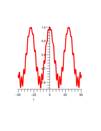
Figure 2: Occupational probability of level (1) as a function of time for $k=0.25$, $\hbar=\omega=1$, $a=0.3$ and $x=1.6$.

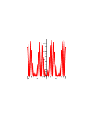
Figure 3: Occupational probability of level (3) as a function of time for the same parameter values as in the previous Figure.

As expected, the time-dependent interaction populates the two other states. See the Figures 2 and 3. Note that level (1) does not go below half occupation.

4 Discussion

We obtained solitary solutions for a three-level system with periodic time-dependent external fields. Two aspects are novel. The external fields are non-linear in the sense that Jacobi’s elliptic functions are used as deformations of the usual harmonic functions. In addition, a full set of special solutions is obtained so that arbitrary initial conditions can be considered.

The additional phase factor $\exp(\mp i\phi(t))$ appearing in the solutions (8, 12) was first considered in [6]. It is not very relevant for the special solutions themselves, but has effect on their superpositions. The function $\sin(\phi(t))$ is plotted in the Figure 4. Its frequency is slightly lower than the frequency $\omega/2\pi$ of the driving field. As a consequence, a low frequency beat appears in the case of a superposition of the special solutions. This is dominantly visible in the Figures 2, 3. For the chosen set of parameters the beat period is about 5 times the frequency of the external field. Note also the frequency doubling by which the exchange of population occurs between levels (2) and (3).

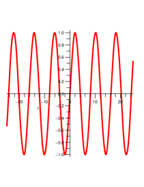
Figure 4: The function $\sin(\phi(t))$ for the same parameter values as in the previous Figures.

Appendix A

The following expressions are used for the generators of SU(3).

$$S_{1} =\frac{1}{2}\left(\begin{array}[]{lcr}0&1&0\\ 1&0&0\\ 0&0&0\\ \end{array}\right),\quad S_{2} =\frac{1}{2}\left(\begin{array}[]{lcr}0&-i&0\\ i&0&0\\ 0&0&0\\ \end{array}\right),$$ (34)

$$S_{3} =\frac{1}{2}\left(\begin{array}[]{lcr}1&0&0\\ 0&-1&0\\ 0&0&0\\ \end{array}\right),\quad S_{4} =\frac{1}{2}\left(\begin{array}[]{lcr}0&0&1\\ 0&0&0\\ 1&0&0\\ \end{array}\right),$$ (41)

$$S_{5} =\frac{1}{2}\left(\begin{array}[]{lcr}0&0&-i\\ 0&0&0\\ i&0&0\\ \end{array}\right),\quad S_{6} =\frac{1}{2}\left(\begin{array}[]{lcr}0&0&0\\ 0&0&1\\ 0&1&0\\ \end{array}\right),$$ (48)

$$S_{7} =\frac{1}{2}\left(\begin{array}[]{lcr}0&0&0\\ 0&0&-i\\ 0&i&0\\ \end{array}\right),\quad S_{8} =\frac{1}{2\sqrt{3}}\left(\begin{array}[]{lcr}1&0&0\\ 0&1&0\\ 0&0&-2\\ \end{array}\right).$$ (55)

Appendix B

The solutions (8, 12) were obtained starting from a known solution of the non-linear von Neumann equation

$$i\hbar\dot{\rho}_{t}=\frac{3}{2}[\{H_{0},\rho_{t}\},\rho_{t}],$$ (56)

where $H_{0}$ is given by

$$H_{0}=\frac{2}{3}\left(\begin{array}[]{lcr}-\mu&0&0\\ 0&\mu&0\\ 0&0&\lambda\end{array}\right).$$ (60)

The three different configurations, vee, ladder, and Lambda, are obtained by taking $\lambda<-\mu<0$, $|\lambda|<\mu$, respectively $\lambda>\mu>0$.

Let $H(t)$ be defined by $H(t)=\frac{3}{2}\{H_{0},\rho_{t}\}$. Then $\rho(t)$ is a solution of the linear von Neumann equation with time-dependent Hamiltonian $H(t)$.

A known solution of the non-linear equation (56) is of the form [5, 8]

$$\rho(t) = \frac{1}{3}{\mathbb{I}}+A\,{\rm cn}\,(\omega t,k)[S_{4}]_{t}+B\,{\rm sn}\,(\omega t,k)[S_{1}]_{t}+C\,{\rm dn}\,(\omega t,k)[S_{7}]_{t}$$ (61)

$$= e^{-(it/\hbar)H_{0}}\left(\begin{array}[]{lcr}\frac{1}{3}&\frac{1}{2}B\,{\rm sn}&\frac{1}{2}A\,{\rm cn}\\ \frac{1}{2}B\,{\rm sn}&\frac{1}{3}&-\frac{i}{2}C\,{\rm dn}\\ \frac{1}{2}A\,{\rm cn}&\frac{i}{2}C\,{\rm dn}&\frac{1}{3}\end{array}\right)e^{(it/\hbar)H_{0}},$$ (65)

The coefficients $A$, $B$, and $C$, are real. They must satisfy the set of conditions

$$\hbar\omega B = \mu AC$$ (66)

$$2\hbar\omega k^{2}C = (\lambda+\mu)AB$$ (67)

$$-2\hbar\omega A = (\lambda-\mu)BC.$$ (68)

This set of equations can be solved in a straightforward manner when $0<|\lambda|<\mu$.

Next, a unitary matrix $V(t)$, satisfying

$$\rho_{t}=V(t)\rho_{0}V(t)^{\dagger}.$$ (69)

is calculated. The fastest way to find $V(t)$ is by first diagonalizing $\rho_{t}$. Note that the eigenvalues of $\rho_{t}$ do not depend on time. They are given by

$$\frac{1}{3}\quad\mbox{ and }\quad\frac{1}{3}\mp\frac{1}{2}T$$ (70)

with $T=\sqrt{A^{2}+C^{2}}$. The result is

$$V(t)=e^{-(it/\hbar)H_{0}}G(t)G(0)^{\dagger}$$ (71)

with

$$G(t)=\frac{1}{\sqrt{2}TR(t)}$$ (72)

$$\times \left(\begin{array}[]{lcr}i\sqrt{2}CR(t)\,{\rm dn}&-AT\,{\rm cn}\,-iBC\,{\rm sn}\,\,{\rm dn}&AT\,{\rm cn}\,-iBC\,{\rm sn}\,\,{\rm dn}\\ -\sqrt{2}AR(t)\,{\rm cn}&AB\,{\rm sn}\,\,{\rm cn}\,+iCT\,{\rm dn}&AB\,{\rm sn}\,\,{\rm cn}\,-iCT\,{\rm dn}\\ \sqrt{2}BR(t)\,{\rm sn}&R(t)^{2}&R(t)^{2}\\ \end{array}\right)$$ (76)

and

$$R(t)=\sqrt{A^{2}\,{\rm cn}\,^{2}+C^{2}\,{\rm dn}\,^{2}}=\sqrt{T^{2}-B^{2}\,{\rm sn}\,^{2}}.$$ (77)

However, $V(t)$ does not necessarily describe the unitary time evolution $U(t)$. But the latter can be related to $V(t)$ by the method of [6]. The knowledge of $U(t)$ implies the time evolution of wavefunctions $\psi(t)$ for arbitrary initial conditions $\psi(t)=U(t)\psi(0)$. It turns out that the special solutions (8, 12) are the columns of the matrix $G(t)$, taken in the interaction picture. Two of the three solutions are multiplied with the time-dependent phase factor $\exp(\mp i\phi(t))$. Finally, note that the conditions (68) are needed during the above derivation but are not required for (8, 12) to hold. They rather are replaced by the single condition (4).

References

• [1] L. Allen and J.H. Eberly, Optical resonance and two-level atoms (Dover publications, 1975, 1987)
• [2] F.T. Hioe, Dynamic symmetries in quantum electronics, Phys. Rev. A 28, 879–886 (1983).
• [3] F.T. Hioe and J.H. Eberly, N-level coherence vector and higher conservation laws in quantum optics and quantum mechanics, Phys. Rev. Lett. 47, 838–841 (1981).
• [4] M. Fleischhauer, A. Imamoglu, and J. P. Marangos, Electromagnetically induced transparency: Optics in coherent media Rev. Mod. Phys. 77, 633–673 (2005).
• [5] M. Czachor, M. Kuna, S.B. Leble, J. Naudts, Nonlinear von Neumann-type equations, in: New Trends in quantum mechanics, H.-D. Doebner, S.T. Ali, M. Keyl, R.F. Werner (eds.) (World Scientific, Singapore, 2000), 209-226
• [6] M. Kuna and J. Naudts, General solutions of quantum mechanical equations of motion with time-dependent Hamiltonians: a Lie algebraic approach, to appear in Rep. Math. Phys.
• [7] C. Cohen-Tannoudji, J. Dupont-Roc, and G. Grynberg, Atom-Photon Interactions (Wiley, New York, 1992).
• [8] Jan Naudts and Maciej Kuna, Special solutions of nonlinear von Neumann equations, arXiv:math-ph/0506020.