Measurement of areas on a sphere using
Fibonacci and latitude–longitude lattices
http://dx.doi.org/10.1007/s11004-009-9257-x)
Abstract
The area of a spherical region can be easily measured by
considering which sampling points of a lattice are located inside
or outside the region. This point-counting technique is frequently
used for measuring the Earth coverage of satellite constellations,
employing a latitude–longitude lattice. This paper analyzes the
numerical errors of such measurements, and shows that they could
be greatly reduced if the Fibonacci lattice were used instead. The
latter is a mathematical idealization of natural patterns with
optimal packing, where the area represented by each point is
almost identical. Using the Fibonacci lattice would reduce the
root mean squared error by at least 40%. If, as is commonly the
case, around a million lattice points are used, the maximum error
would be an order of magnitude smaller.
Keywords: Spherical grid; Golden ratio; Equal-angle grid;
Non-standard grid; Fibonacci grid; Phyllotaxis
1 Introduction
The area of a region is easy to measure, without explicitly considering its boundaries, by determining which points of a lattice are inside or outside the region. This point-counting method is commonly applied to estimating areas on a plane [5, 33, 29, 27, 3]. A related issue is how to approximate the region boundaries from this sampling [4].
Point-counting on the sphere is commonly used for estimating the Earth coverage of satellite constellations [36, 22], the fraction of the Earth’s surface efficiently seen by one or more satellites. In the simplest case, each satellite covers a circular region (cap), so the constellation covers a complex set of isolated and/or overlapping caps [36]. Similarly, some maps designed for global earthquake forecasting depict earthquake-prone regions as complex sets of up to tens of thousands of caps [41, 35, 24]. To assess these forecasts it is necessary to measure the fraction of the Earth’s area covered by these regions [35].
Analytical solutions exist if the spherical region has a known, regular or polygonal shape [38, 8, 63]. The area of a set of caps on the sphere has a complex analytical solution [36], which unfortunately does not indicate whether any particular location on the surface of the sphere is covered.
The numerical error of point counting should ideally decrease rapidly as the lattice density increases. Numerous works deal with errors on the plane [5, 33, 29, 27, 3]. Some particular cases using latitude–longitude lattices were analyzed elsewhere [36]. In automated counting, the computation time is directly proportional to the number of lattice points. Satellite constellation coverage [53] or the areas marked on rapidly-updated earthquake forecasting maps [24] need continuous monitoring, implying a trade-off between accuracy and computational load. Thus it is important to find lattices able to measure areas as efficiently as possible.
On the plane, the regular hexagonal lattice provides optimal sampling [12]. On the sphere, it is impossible to arrange regularly more than 20 points (the vertices of a dodecahedron), and the optimum configuration of a large number of points is problem-specific [60, 12, 75, 25]. For optimal point-counting, the area represented by every point should be almost the same.

Traditionally, the latitude–longitude lattice is used for measuring Earth coverage [36, 53, 22]. However, it is very inhomogeneous (Fig. 1), requiring non-uniform weighting of the point contributions. Also, its number of points is restricted by geometrical constraints.
The Fibonacci lattice is a particularly appealing alternative [15, 16, 17, 23, 65, 42, 66, 67, 68, 76, 52, 28, 56, 55]. Being easy to construct, it can have any odd number of points [68], and these are evenly distributed (Fig. 1) with each point representing almost the same area. For the numerical integration of continuous functions on a sphere, it has distinct advantages over other lattices [28, 56].
This paper demonstrates that for measuring the areas of spherical caps, the Fibonacci lattice is much more efficient than its latitude–longitude counterpart. After describing both lattices (Sects. 2 and 3), it is explained how to use them for measuring cap areas (Sect. 4) and how the error of this measurement is assessed (Sect. 5). The error results obtained from an extensive Monte Carlo simulation are described, and to some extent explained analytically (Sect. 6). The conclusions are set out in the final section.
2 Latitude–Longitude Lattice
The latitude–longitude lattice is the set of points located at the intersections of a grid of meridians and parallels, separated by equal angles of latitude and longitude (Fig. 1). This is the “latitude–longitude grid” [68, 75] or “equal-angle grid” [25]. The points concentrate towards the poles, due to the converging meridians, resulting in high anisotropy.
The number of points, , depends on the angular spacing, , between grid lines. Since with ,
| (1) |
That is the number of meridians times the number of parallels , plus the two poles. Frequently, to evaluate satellite coverage, [22] , so more than a million points are used.
3 Fibonacci Lattice
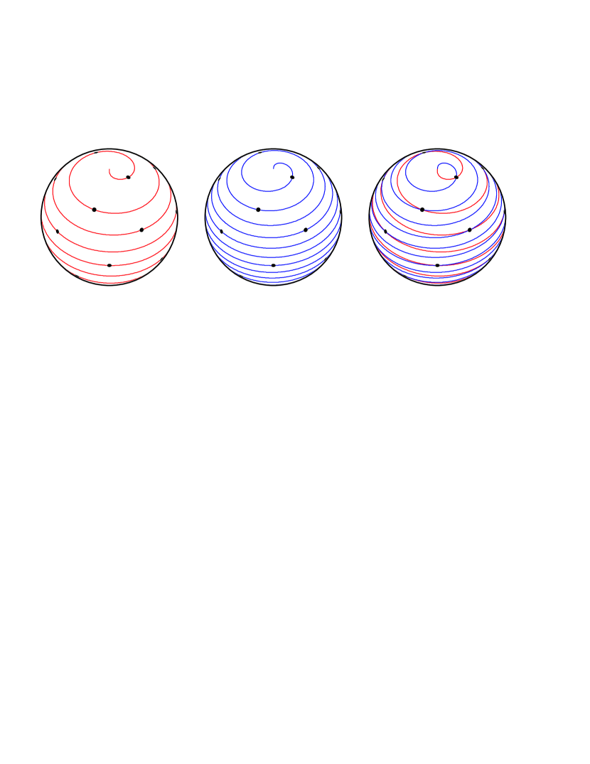
The points of the Fibonacci lattice are arranged along a tightly wound generative spiral, with each point fitted into the largest gap between the previous points (Fig. 2). This spiral is not apparent (Fig. 1) because consecutive points are spaced far apart from each other. The most apparent spirals join the points closest to each other, and form crisscrossing sets [68]. The points are evenly spaced in a very isotropous way.
The next subsections describe how to construct the lattice used in this paper, and the history of the Fibonacci lattice in various research fields.
3.1 Lattice Construction
The Fibonacci lattice is named after the Fibonacci ratio. The Fibonacci sequence was discovered in ancient India [62, 40] and rediscovered in the middle ages by Leonardo Pisano, better known by his nickname Fibonacci [61]. Each term of the sequence, from the third onwards, is the sum of the previous two: 0, 1, 1, 2, 3, 5, 8, 13, 21, Given two consecutive terms, and , a Fibonacci ratio is . As first proved by Robert Simson in 1753 [73], this quotient, as , quickly approaches the golden ratio, defined as .
The Fibonacci lattice differs from other spiral lattices on the sphere [72, 39, 57, 60, 11, 6, 30] in that the longitudinal turn between consecutive points along the generative spiral is the golden angle, , or its complementary, . Some lattice versions replace by its rational approximant, a Fibonacci ratio.
The golden angle optimizes the packing efficiency of elements in spiral lattices [58, 59]. This is because the golden ratio is the most irrational number [73], so periodicities or near-periodicities in the spiral arrangement are avoided, and clumping of the lattice points never occurs [58, 15, 54, 34, 28].
The lattice version used here [68] is probably the most homogeneous one. It is generated with a Fermat spiral (also known as the cyclotron spiral) [70, 15, 17], which embraces an equal area per equal angle turn, so the area between consecutive sampling points, measured along the spiral, is always the same [68]. Also, its first and last points are offset from the poles, leading to a more homogeneous polar arrangement [56, 68] than in other versions [65, 42, 52, 28, 56]. When a Fibonacci ratio is used [65, 42, 52, 28], the number of lattice points is , where is a term of the Fibonacci sequence. The lattice used here is instead based on the golden ratio and can have any odd number of points.
To elaborate the lattice [68], let be any natural number. Let the integer range from to . The number of points is
| (2) |
and the spherical coordinates, in radians, of the th point are:
| (3) | |||||
| (4) |
This pseudocode provides the geographical coordinates in degrees:
For , Do {
If , then
If , then
} End Do
Here, arcsin returns a value in radians, while
returns the remainder when is divided by , removing the
extra turns of the generative spiral. For example, . The last two lines keep the longitude
range from to .
Every point of this lattice is located at a different latitude, providing a more efficient sampling than the latitude–longitude lattice. The middle point, , is placed at the equator ( and ). Each of the other points with , has a centrosymmetric one with . The lattice as a whole is not centrosymmetric.
The longitudinal turn between consecutive lattice points along the spiral (Eq. 4) is the complementary of the golden angle [66, 68]. To use the golden angle instead, we can substitute Eq. 4 by
| (5) |
With Eq. 4, the spiral progresses eastwards, while the minus sign of Eq. 5 indicates a westward progression.
A remark not found elsewhere is that the lattice points are placed at the intersections between these Fermat spirals of opposite chirality, except at the poles (Fig. 2). For drawing the spirals, is made continuous in Eqs. 3, 4 and 5, and ranges from to . The term accounts for the polar offset [56, 68].
3.2 Lattice History
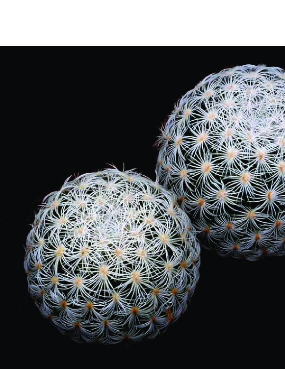
The Fibonacci lattice is a mathematical idealization of patterns of repeated plant elements, such as rose petals, pineapple scales, or sunflower seeds (Fig. 3). The study of these arrangements is known as Phyllotaxis [54, 34, 1, 43]. The Bravais brothers [10] were the first to describe them using a spiral lattice on a cylinder. They argued that the most common angle turn between consecutive elements along this spiral in plants is the golden angle. The latter provides optimum packing [58, 59], maximizing the exposure to light, rain and insects for pollination [46]. Structures in cells and viruses also follow this pattern [20]. In some experiments, elements are spontaneously ordered on roughly hemispherical Fibonacci lattices, because the system tends to minimize the strain energy [45] or to avoid periodic organization [18].
Unwrapping the cylindrical Fibonacci lattice produces a flat one [10, 28, 68], frequently used for numerical integration [77, 50, 51, 64].
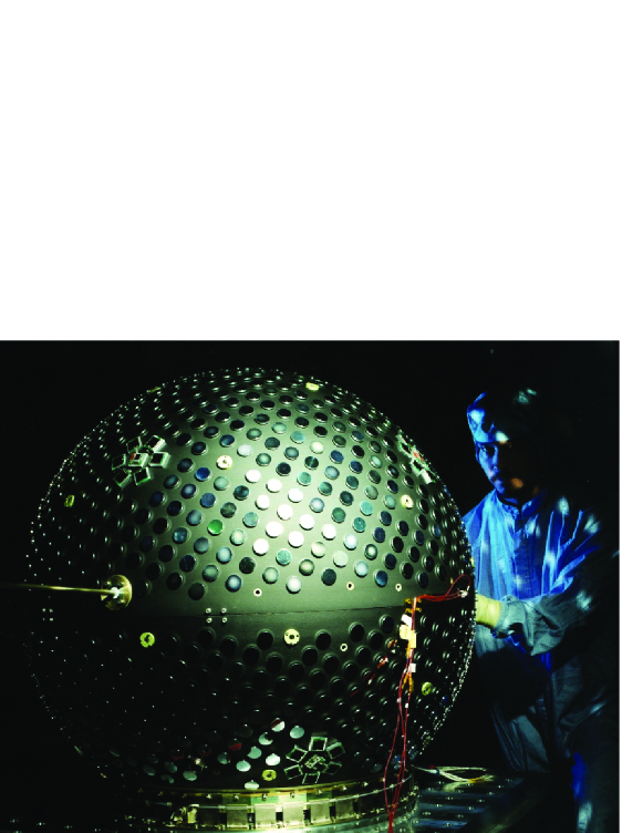
Projecting the cylindrical Fibonacci lattice to the sphere generates the spherical version [28, 68]. This can be generalized to arbitrary surfaces of revolution [59, 17]. The first graphs of spherical Fibonacci lattices used, as here, the golden ratio and a Fermat spiral [15, 16, 17]. A version based on the Fibonacci ratio is used in the modelling of complex molecules [71, 65, 42]. In this case [65, 42], a “+” sign in the formula for the longitude should be substituted by “” (D. Svergun, personal communication, 2009). Versions with the golden ratio serve to simulate plants realistically [23] and to design golf balls [76]. The latter method was used by Douglas C. Winfield (B. Moore and D. C. Winfield, personal communication, 2009) in the Starshine-3 satellite (Fig. 4).
4 Area Measurement
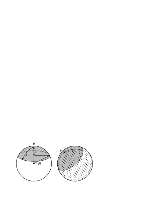
The area measurement starts by finding which points of the lattice are inside the considered region. This is expressed by a Boolean function , such that if the th point is inside, and otherwise [36]. If the region is a cap with radius , it suffices to measure , the shortest distance (great-circle distance) between the sampling point and the cap centre (Fig. 5):
| (6) |
Each lattice point must be assigned a weight, , proportional to the area it represents. Then the estimate, , of the region area , is measured considering the sphere area, , and summing the contribution of all points of the lattice:
| (7) |
The weights depend on the lattice type, as described below.
4.1 Weights in the Latitude–Longitude Lattice
The weights should be inversely proportional to the point density, which here increases towards the poles (Fig. 1). The linear spacing between parallels is constant. The length of a parallel is , where is the sphere radius. In any parallel there is the same number of lattice points (), so their density is inversely proportional to [36, 69]:
| (8) |
4.2 Weights in the Fibonacci lattice
Thanks to the even distribution of points in this lattice, the same weight can be assumed for all of them [56, 68], namely
| (9) |
Each point represents the area corresponding to its Voronoi cell (Thiessen polygon). This is the region of positions closer to the corresponding lattice point than to any other [21, 49]. Using the exact area of each Voronoi cell as weight for its lattice point [2] would improve the area measurement only slightly. The average cell area equals . Here, regardless of , only the areas of less than ten cells, located at the polar regions, differ by more than from this value [68]. As increases, proportionally fewer cells depart significantly from the average area. Unlike the latitude–longitude lattice, the homogeneity of the Fibonacci lattice improves with the number of points.
5 Error Assessment
This section details how to assess the error involved in measuring the area of spherical caps placed at random on the sphere. A good way to measure the homogeneity of a spherical lattice is to compare the proportion of lattice points in spherical regions with the normalized areas of the regions [13]. For this task, it is natural to use spherical caps [60, 14, 9], which moreover appear in the applications mentioned in the introduction.
The area of a spherical cap (see Fig. 5) is:
| (10) |
The normalized cap area is:
| (11) |
where is the sphere area.
The absolute error of measuring a single cap is the absolute difference between the estimated fraction and the actual one:
| (12) |
This depends on the lattice type, the number of points, and the size and location of the cap. If , the cap gets its fair share of weighted lattice points. If , . A plane cuts the sphere into two complementary caps. For any cap, is the same as for the complementary cap with area , so it suffices to consider caps not larger than a hemisphere ().
The error is characterized here numerically using a Monte Carlo method. In each particular realization, a cap is randomly placed. Every point of the sphere has the same probability of becoming the cap centre, , with coordinates:
| (13) | |||||
| (14) |
Here is a random number, chosen with uniform probability in the range , independently for each equation. The area of this th cap is estimated, and its corresponding error is .
The process is repeated for a total of independently located caps of the same size, providing a sample of values of . The root mean squared error is [73]:
| (15) |
The supremum error in Eq. 12 for caps of any size, for a given lattice type and , using , is the “spherical cap discrepancy” [60, 14, 9]. It cannot be determined exactly with a Monte Carlo simulation because it might result from a cap size not used, or a location not sampled. However, it is unfortunately difficult to compute explicitly [14]. The maximum measured for the Fibonacci lattice is a lower bound to its spherical cap discrepancy.
6 Results
This section details the maximum errors and root mean squared errors measured with the Monte Carlo simulation detailed in the previous section.
Thirteen lattice configurations of each type, from to , were analyzed. The chosen values of increase in logarithmic steps, as accurately as possible (). It is impossible to use identical for both lattices because is odd in the Fibonacci lattice but even in the latitude–longitude lattice. Moreover, there are considerably fewer possible values of in the latter. For each configuration, 200 different cap sizes were used: from to in steps of . To obtain smooth results, was chosen for each cap size and lattice configuration.
In total, 312 million caps were measured (2 lattice types 13 values of 200 cap sizes 60,000 caps). After optimization, the calculation took 43 days of CPU time using 2.8 GHz, 64-bit processors.
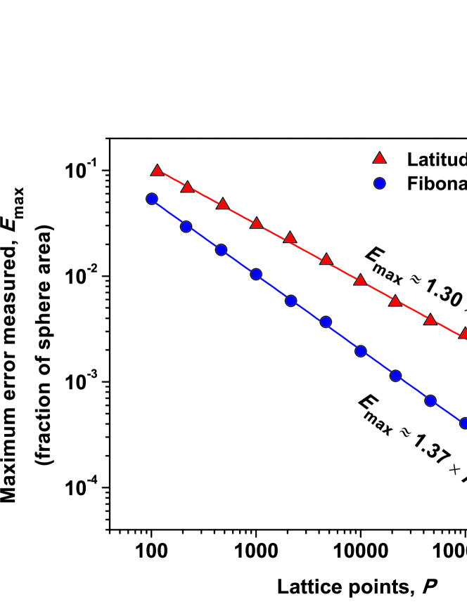
The maximum measured, for caps of any size and location, is represented in Fig. 6. For the Fibonacci lattice, it is much lower and decays faster than for the latitude–longitude lattice, despite the non-uniform weighting of points of the latter.
The rmse depends on the lattice type, number of points and cap size, as shown in Fig. 7. Because of the symmetry of the latitude–longitude lattice, any hemispherical cap covers one half of the points of the lattice, and (thanks to the point weighs) the estimation is perfect ( and rmse). This exception aside, the rmse tends to increase with the cap area, in a non-trivial way, which is more complex for the latitude–longitude lattice than for the Fibonacci lattice.

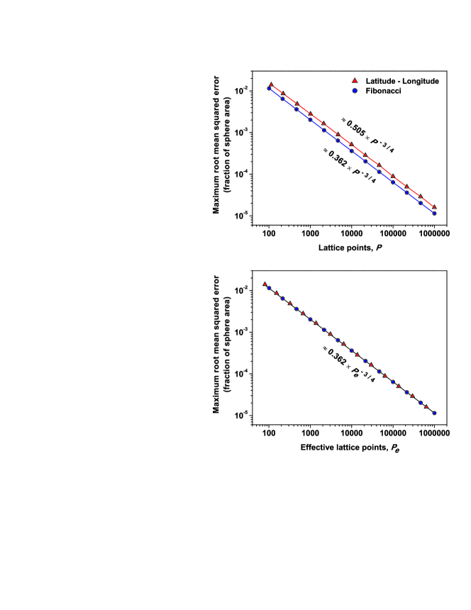
Figure 8 (top) shows the maximum values of rmse of each curve. They follow parallel power laws:
| (16) |
with for the latitude–longitude lattice, and for the Fibonacci lattice. Interpolating for the same , the rmsemax would be larger in the latitude–longitude lattice.
6.1 Analytical Approach to the Root Mean Squared Error
The scaling shown in Fig. 8 can be explained using arguments from similar problems in the plane [37, 31, 32]. The number of points of a regular square lattice enclosed by a sufficiently smooth, closed curve placed at random can be expressed as [32]:
| (17) |
where is the area enclosed by the curve, is the inverse to the lattice spacing, and is the discrepancy. The nominal spacing of a spherical lattice is [68]. Assuming that the Fibonacci lattice is regular enough,
| (18) |
Substituting this into Eq. 17,
| (19) |
Dividing all the terms of this equation by ,
| (20) |
In the planar case, the root mean squared of , rms, is proportional to [37, 31, 32]. Extrapolating this fact, we obtain the scaling observed in the Monte Carlo simulation:
| (21) |
In the latitude–longitude lattice, the same scaling holds if we consider its smaller sampling efficiency. The latter may be measured with the denominator of Eq. 7. This is the number of points of a homogeneous lattice that would do the same work, and is up to smaller than in the range of considered here. If Fig. 8 is plotted using these effective points in the abscissas, the same fit suffices for both lattice types (Fig. 8, bottom).
If the sampling points were placed at random, the rmse would decrease more slowly, as [7].
7 Conclusions
This paper analyzes the errors involved in measuring the areas of spherical caps using lattices of sampling points: the latitude–longitude lattice (classically used for this task), and a Fibonacci lattice [68]. The latter has low anisotropy, is easy to construct, and is shown to result from the intersection of two generative spirals (Fig. 2). A a review of the literature (Sect. 3.2) reveals successful applications of this spherical lattice since the 1980s.
If the Fibonacci lattice were used instead of its latitude–longitude counterpart, the area measurement would be more efficient, allowing a significant reduction of the computation time. For approximately the same number of lattice points, the maximum root mean squared error would be about 40% smaller (Fig. 8). The maximum errors would be also smaller, and would decay faster with the number of points (Fig. 6). If about a million points were used, as is commonly the case [22], the maximum error would be an order of magnitude smaller (Fig. 6).
It is also found that the maximum root mean squared error obeys a single scaling relation when the sampling efficiency is taken into account (Fig. 8). This is partially explained using arguments from similar problems on the plane [37, 31, 32].
The area estimate depends also on the orientation of the sampling lattice, especially if the latter has high anisotropy. The difference may be assessed [28] by rotating the lattice [26]. Such an issue is not relevant in the case analyzed here because the caps were placed at random with uniform probability over the spherical surface.
8 Acknowledgements
I thank John H. Hannay, Gil Moore, Dimitri Svergun, Richard Swinbank, John Vasquez, Gert Vriend and Douglas C. Winfield for clarifying different aspects of their work. The results were calculated using the supercomputing facilities of the Institute of Biocomputing and Physics of Complex Systems (BIFI, University of Zaragoza, Spain). Lattice maps were produced with Generic Mapping Tools [74]. I am also grateful to an anonymous reviewer for offering insightful and encouraging comments.
References
- [1] Adler, I.; Barabe, D. & Jean, R. V. (1997) A history of the study of phyllotaxis. Annals of Botany, 80 (3), 231–244. Doi:10.1006/anbo.1997.0422
- [2] Ahmad, R.; Deng, Y.; Vikram, D. S.; Clymer, B.; Srinivasan, P.; Zweier, J. L. & Kuppusamy, P. (2007) Quasi Monte Carlo-based isotropic distribution of gradient directions for improved reconstruction quality of 3D EPR imaging. Journal of Magnetic Resonance, 184 (2), 236–245. Doi:10.1016/j.jmr.2006.10.008
- [3] Baddeley, A. & Jensen, E. B. V. (2004) Stereology for Statisticians. CRC Press, Boca Raton, Florida. 416 pp.
- [4] Barclay, M. & Galton, A. (2008) Comparison of region approximation techniques based on Delaunay triangulations and Voronoi diagrams. Computers, Environment and Urban Systems, 32 (4), 261–267. Doi:10.1016/j.compenvurbsys.2008.06.003
- [5] Bardsley, W. E. (1983) Random error in point counting. Mathematical Geology, 15 (3), 469–475. Doi:10.1007/BF01031293
- [6] Bauer, R. (2000) Distribution of points on a sphere with application to star catalogs. Journal of Guidance, Control and Dynamics, 23 (1), 130–137.
- [7] Bevington, P. R. & Robinson, D. K. (1992) Data Reduction and Error Analysis for the Physical Sciences, 2nd edn. McGraw Hill, Boston, 328 pp.
- [8] Bevis, M. & Cambareri, G. (1987) Computing the area of a spherical polygon of arbitrary shape. Mathematical Geology, 19 (4), 335–346. Doi:10.1007/BF00897843
- [9] Brauchart, J. S. (2004) Invariance principles for energy functionals on spheres. Monatshefte für Mathematik, 141 (2), 101–117. Doi:10.1007/s00605-002-0007-0
- [10] Bravais, L. & Bravais, A. (1837) Essai sur la disposition des feuilles curvisériées. Annales des Sciences Naturelles 7, 42–110 & plates 2–3.
- [11] Chukkapalli, G.; Karpik, S. R. & Ethier, C. R. (1999) A scheme for generating unstructured grids on spheres with application to parallel computation. Journal of Computational Physics, 149 (1), 114–127. Doi:10.1006/jcph.1998.6146
- [12] Conway, J. H. & Sloane, N. J. A. (1998) Sphere Packings, Lattices and Groups, 3rd edn. Springer-Verlag, New York, 703 pp.
- [13] Cui, J. & Freeden, W. (1997) Equidistribution on the sphere. SIAM Journal on Scientific Computing, 18 (2), 595–609. Doi:10.1137/S1064827595281344
- [14] Damelin, S. B. & Grabner, P. J. (2003) Energy functionals, numerical integration and asymptotic equidistribution on the sphere. Journal of Complexity, 19 (3), 231–246. Doi:10.1016/S0885-064X(02)00006-7 [Corrigendum in 20 (6), 883–884. Doi:10.1016/j.jco.2004.06.003]
- [15] Dixon, R. (1987) Mathographics. Basil Blackwell, Oxford, England, 224 pp.
- [16] Dixon, R. (1989) Spiral phyllotaxis. Computers and Mathematics with Applications, 17 (4–6), 535–538.
- [17] Dixon, R. (1992) Green spirals. In: Hargittai, I. & Pickover, C. A. (Eds.) Spiral Symmetry. World Scientific, Singapore, pp. 353–368.
- [18] Douady, S. & Couder, Y. (1992) Phyllotaxis as a physical self-organized growth process. Physical Review Letters 68 (13), 2098–2101. Doi:10.1103/PhysRevLett.68.2098
- [19] Earle, M. A. (2006) Sphere to spheroid comparisons. The Journal of Navigation 59 (3), 491–496. Doi:10.1017/S0373463306003845
- [20] Erikson, R. O. (1973) Tubular packing of spheres in biological fine structure. Science, 181 (4101), 705–716. Doi:10.1126/science.181.4101.705
- [21] Evans, D. G. & Jones, S. M. (1987) Detecting Voronoi (area-of-influence) polygons. Mathematical Geology, 19 (6), 523–537. Doi:10.1007/BF00896918
- [22] Feng, S.; Ochieng, W. Y. & Mautz, R. (2006) An area computation based method for RAIM holes assessment. Journal of Global Positioning Systems, 5 (1–2), 11–16.
- [23] Fowler, D. R.; Prusinkiewicz, P. & Battjes, J. (1992) A collision-based model of spiral phyllotaxis. ACM SIGGRAPH Computer Graphics, 26 (2), 361–368. Doi:10.1145/142920.134093
- [24] González, Á. (2009) Self-sharpening seismicity maps for forecasting earthquake locations. In: Abstracts of the Sixth International Workshop on Statistical Seismology, Tahoe City, California, 16–19 April 2009. http://www.scec.org/statsei6/posters.html [Last accessed: November 16th, 2009]
- [25] Gregory, M. J.; Kimerling, A. J; White, D. & Sahr, K. (2008) A comparison of intercell metrics on discrete global grid systems. Computers, Environment and Urban Systems, 32 (3), 188–203. Doi:10.1016/j.compenvurbsys.2007.11.003
- [26] Greiner, B. (1999) Euler rotations in plate-tectonic reconstructions. Computers and Geosciences, 25 (3), 209–216. Doi:10.1016/S0098-3004(98)00160-5
- [27] Gundersen, H. J. G.; Jensen, E. B. V.; Kiêu, K. & Nielsen, J. (1999) The efficiency of systematic sampling in stereology – reconsidered. Journal of Microscopy, 193 (3), 199-211. Doi:10.1046/j.1365-2818.1999.00457.x
- [28] Hannay, J. H. & Nye, J. F. (2004) Fibonacci numerical integration on a sphere. Journal of Physics A: Mathematical and General, 37 (48), 11591–11601. Doi:10.1088/0305-4470/37/48/005
- [29] Howarth, R. J. (1998) Improved estimators of uncertainty in proportions, point-counting, and pass-fail test results. American Journal of Science, 298 (7), 594–607.
- [30] Hüttig, C. & Stemmer, K. (2008) The spiral grid: a new approach to discretize the sphere and its application to mantle convection. Geochemistry, Geophysics, Geosystems 9 (2), Q02018. Doi:10.1029/2007GC001581
- [31] Huxley, M. N. (1987) The area within a curve. Proceedings of the Indian Academy of Sciences (Mathematical Sciences), 97 (1–3), 111–116. Doi:10.1007/BF02837818
- [32] Huxley, M. N. (2003) Exponential sums and lattice points III. Proceedings of the London Mathematical Society, 87 (3), 591–609. Doi:10.1112/S0024611503014485
- [33] Jarái, A.; Kozák, M. & Rózsa, P. (1997) Comparison of the methods of rock-microscopic grain-size determination and quantitative analysis. Mathematical Geology, 29 (8), 977–991. Doi:10.1023/A:1022305518696
- [34] Jean, R. V. (1994) Phyllotaxis: A Systemic Study of Plant Pattern Morphogenesis. Cambridge University Press, Cambridge, UK, 400 pp.
- [35] Kafka, A. L. (2007) Does seismicity delineate zones where future large earthquakes are likely to occur in intraplate environments? In: Stein, S. & Mazzotti, S. (Eds.) Continental Intraplate Earthquakes: Science, Hazard, and Policy Issues. Geological Society of America Special Paper 425, Boulder, Colorado, pp. 35–48. Doi:10.1130/2007.2425(03)
- [36] Kantsiper, B. & Weiss, S. (1998) An analytic approach to calculating Earth coverage. Advances in the Astronautical Sciences, 97, 313–332.
- [37] Kendall, D. G. (1948) On the number of lattice points inside a random oval. The Quarterly Journal of Mathematics (Oxford), 19 (1), 1–26. Doi:10.1093/qmath/os-19.1.1
- [38] Kimerling, A. J. (1984) Area computation from geodetic coordinates on the spheroid. Surveying and Mapping, 44 (4), 343–351.
- [39] Klíma, K.; Pick, M. & Pros, Z. (1981) On the problem of equal area block on a sphere. Studia Geophysica et Geodaetica (Praha), 25 (1), 24–35. Doi:10.1007/BF01613559
- [40] Knuth, D. E. (1997) Art of Computer Programming, Volume 1: Fundamental Algorithms, 3rd edn. Addison-Wesley, Reading, Massachusetts, 672 pp.
- [41] Kossobokov, V. & Shebalin, P. (2003) Earthquake prediction. In: Keilis-Borok, V. I. & Soloviev, A. A. (Eds.) Nonlinear Dynamics of the Lithosphere and Earthquake Prediction. Springer, Berlin, pp. 141–207. [References in pp. 311–332]
- [42] Kozin, M. B.; Volkov, V. V. & Svergun, D. I. (1997) ASSA, a program for three-dimensional rendering in solution scattering from biopolymers. Journal of Applied Crystallography, 30 (5), 811–815. Doi:10.1107/S0021889897001830
- [43] Kuhlemeier, C. (2007) Phyllotaxis. Trends in Plant Science, 12 (4), 143–150. Doi:10.1016/j.tplants.2007.03.004
- [44] Lean, J. L.; Picone, J. M.; Emmert, J. T. & Moore, G. (2006) Thermospheric densities derived from spacecraft orbits: application to the Starshine satellites. Journal of Geophysical Research, 111 (4), A04301. Doi:10.1029/2005JA011399
- [45] Li, C.; Zhang, X. & Cao, Z. (2005) Triangular and Fibonacci number patterns driven by stress on core/shell microstructures. Science, 309 (5736), 909–911. Doi:10.1126/science.1113412
- [46] Maciá, E. (2006) The role of aperiodic order in science and technology. Reports on Progress in Physics, 69 (2), 397–441. Doi:10.1088/0034-4885/69/2/R03
- [47] Maley, P. D.; Moore, R. G. & King, D. J. (2002) Starshine: a student-tracked atmospheric research satellite. Acta Astronautica, 51 (10), 715–721. Doi:10.1016/S0094-5765(02)00021-8
- [48] Michalakes, J. G.; Purser, R. J. & Swinbank, R. (1999) Data structure and parallel decomposition considerations on a Fibonacci grid. In: Preprints of the 13th Conference on Numerical Weather Prediction, Denver, 13-17 September 1999. American Meteorological Society, pp. 129–130.
- [49] Na, H. S.; Lee, C. N. & Cheong, O. (2002) Voronoi diagrams on the sphere. Computational Geometry – Theory and Applications, 23 (2), 183–194. Doi:10.1016/S0925-7721(02)00077-9
- [50] Niederreiter, H. (1992) Random Number Generation and Quasi-Monte Carlo Methods. Society for Industrial and Applied Mathematics, Philadelphia, 247 pp.
- [51] Niederreiter, H. & Sloan, I. H. (1994) Integration of nonperiodic functions of two variables by Fibonacci lattice rules. Journal of Computational and Applied Mathematics, 51 (1), 57–70. Doi:10.1016/0377-0427(92)00004-S
- [52] Nye, J. F. (2003) A simple method of spherical near-field scanning to measure the far fields of antennas or passive scatterers. IEEE Transactions on Antennas and Propagation, 51 (8), 2091–2098. Doi:10.1109/TSP.2003.815442
- [53] Ochieng, W. Y.; Sheridan, K. F.; Sauer, K. & Han, X. (2002) An assessment of the RAIM performance of a combined Galileo/GPS navigation system using the marginally detectable errors (MDE) algorithm. GPS Solutions 5 (3), 42–51. Doi:10.1007/PL00012898
- [54] Prusinkiewicz, P. & Lindenmayer, A. (1990) The Algorithmic Beauty of Plants. Springer-Verlag, New York, 228 pp.
- [55] Purser, R. J. (2008) Generalized Fibonacci grids: a new class of structured, smoothly adaptive multi-dimensional computational lattices. Office Note 455, National Centers for Environmental Prediction, Camp Springs, Maryland, USA, 37 pp.
- [56] Purser, R. J. & Swinbank, R. (2006) Generalized Euler-Maclaurin formulae and end corrections for accurate quadrature on Fibonacci grids. Office Note 448, National Centers for Environmental Prediction, Camp Springs, Maryland, USA, 19 pp.
- [57] Rakhmanov, E. A.; Saff, E. B. & Zhou, Y. M. (1994) Minimal discrete energy on the sphere. Mathematical Research Letters, 1 (6), 647–662.
- [58] Ridley, J. N. (1982) Packing efficiency in sunflower heads. Mathematical Biosciences, 58 (1), 129–139. Doi:10.1016/0025-5564(82)90056-6
- [59] Ridley, J. N. (1986) Ideal phyllotaxis on general surfaces of revolution. Mathematical Biosciences, 79 (1), 1–24. Doi:10.1016/0025-5564(86)90013-1
- [60] Saff, E. B. & Kuijlaars, A. B. J. (1997) Distributing many points on a sphere. The Mathematical Intelligencer, 19 (1), 5–11. Doi:10.1007/BF03024331
- [61] Sigler, L. E. (2002) Fibonacci’s Liber Abaci: a Translation into Modern English of Leonardo Pisano’s Book of Calculation. Springer, New York, 636 pp.
- [62] Singh, P. (1985) The so-called Fibonacci numbers in ancient and medieval India. Historia Mathematica, 12 (3), 229–244. Doi:10.1016/0315-0860(85)90021-7
- [63] Sjöberg, L. E. (2006) Determination of areas on the plane, sphere and ellipsoid. Survey Review, 38 (301), 583–593.
- [64] Sloan, I. H. & Joe, S. (1994) Lattice Methods for Multiple Integration. Oxford University Press, Oxford, UK, 256 pp.
- [65] Svergun, D. I. (1994) Solution scattering from biopolymers: advanced contrast-variation data analysis. Acta Crystallographica, A50 (3), 391–402. Doi:10.1107/S0108767393013492
- [66] Swinbank, R. & Purser, R. J. (1999) Fibonacci grids. In: Preprints of the 13th Conference on Numerical Weather Prediction, Denver 13–17 September 1999. American Meteorological Society, pp. 125–128.
- [67] Swinbank, R. & Purser, R. J. (2006a) Standard test results for a shallow water equation model on the Fibonacci grid. Forecasting Research Technical Report 480, Met Office, Exeter, UK, 12 pp.
- [68] Swinbank, R. & Purser, R. J. (2006b) Fibonacci grids: a novel approach to global modelling. Quarterly Journal of the Royal Meteorological Society, 132 (619), 1769–1793. Doi:10.1256/qj.05.227
- [69] Van den Dool, H. M. (2007) Empirical Methods in Short-Term Climate Prediction. Oxford University Press, Oxford, UK, 240 pp.
- [70] Vogel, H. (1979) A better way to construct the sunflower head. Mathematical Biosciences, 44 (3–4), 179–189. Doi:10.1016/0025-5564(79)90080-4
- [71] Vriend, G. (1990) WHAT IF: a molecular modeling and drug design program. Journal of Molecular Graphics, 8 (1), 52–56. Doi:10.1016/0263-7855(90)80070-V
- [72] Weiller, A. R. (1966) Probleme de l’implantation d’une grille sur une sphere, deuxième partie. Bulletin Géodésique, 80 (1), 99–111. Doi:10.1007/BF02527041
- [73] Weisstein, E. W. (2002) CRC Concise Encyclopedia of Mathematics CD-ROM, 2nd edn. CRC Press, Boca Raton, Florida, 3252 pp.
- [74] Wessel, P. & Smith, W. H. F. (1998) New, improved version of Generic Mapping Tools released. Eos, Transactions, American Geophysical Union, 79 (47), 579.
- [75] Williamson, D. L. (2007) The evolution of dynamical cores for global atmospheric models. Journal of the Meteorological Society of Japan, 85B, 241–269.
- [76] Winfield, D. C. & Harris, K. M. (2001) Phyllotaxis-Based Dimple Patterns. Patent number WO 01/26749 Al. World Intellectual Property Organization, Geneva, Switzerland.
- [77] Zaremba, S. K. (1966) Good lattice points, discrepancy, and numerical integration. Annali di Matematica Pura ed Applicata, 73 (1), 293–317. Doi:10.1007/BF02415091