Preface

C. Balázs and D. Carter csaba.balazs@sci.monash.edu.audaniel.carter@sci.monash.edu.auBrookes Institute for Advanced Studies,
Bøgevej 6, 2900 Hellerup, DenmarkDepartment of Physics, FMF, University of Ljubljana,
Jadranska 19, 1000 LjubljanaUniversidad de Zacatecas
Ap. Postal 636, Suc. 3 Cruces, C. P. 98064
Zacatecas, Zac., MéxicoUniversidad de Zacatecas, Apartado Postal 636, Suc. 3 Cruces
Zacatecas 98064, Zac., México
URL: http://planck.reduaz.mx/ṽaleri/
e-mail address: valeri@fisica.uaz.edu.mxDepartamento de Física, Escuela Superior de Física y Matemáticas, I.P.N.,
U. P. ”Adolfo López Mateos”. C. P. 07738, México, D.F., México¹Moscow Engineering Physics Institute (National Nuclear Research University), 115409 Moscow, Russia
² Centre for Cosmoparticle Physics ”Cosmion” 115409 Moscow, Russia
³ APC laboratory 10, rue Alice Domon et Léonie Duquet
75205 Paris Cedex 13, FranceSCAT, Oslo, Norway¹ Department of Physics, FMF, University of Ljubljana,
Jadranska 19,Ljubljana, 1000
² Department of Physics, Niels Bohr Institute,
Blegdamsvej 17, Copenhagen, DK-2100Department of Physics, FMF, University of Ljubljana,
Jadranska 19, 1000 Ljubljana, Slovenia
http://www.fmf.uni-lj.si14U
155 E 34 Street
New York, NY 10016 (http://viavca.in2p3.fr/bled_09.html)¹ Department of Physics, FMF, University of Ljubljana,
Jadranska 19,Ljubljana, 1000
² Department of Physics, Niels Bohr Institute,Blegdamsvej 17, Copenhagen, DK-2100Department of Physics, FMF, University of Ljubljana,
Jadranska 19,Ljubljana, 1000Centre for Cosmoparticle Physics Cosmion, 115409 Moscow, Russia;
Moscow Engineering Physics Institute (National Nuclear Research University), 115409 Moscow, Russia
APC laboratory 10, rue Alice Domon et Léonie Duquet
75205 Paris Cedex 13, France¹Departamento de Física, Escuela Superior de Física y Matemáticas, I.P.N.,
U. P. ”Adolfo López Mateos”. C. P. 07738, México, D.F., México
²Department of Physics, FMF, University of Ljubljana,
Jadranska 19,Ljubljana, 100014U
155 E 34 Street
New York, NY 10016 ¹Moscow Engineering Physics Institute (National Nuclear Research University), 115409 Moscow, Russia
² Centre for Cosmoparticle Physics ”Cosmion” 125047 Moscow, Russia
³ APC laboratory 10, rue Alice Domon et Léonie Duquet
75205 Paris Cedex 13, France

The series of workshops on ”What Comes Beyond the Standard Model?” started in 1998 with the idea of organizing a real workshop, in which participants would spend most of the time in discussions, confronting different approaches and ideas. The picturesque town of Bled by the lake of the same name, surrounded by beautiful mountains and offering pleasant walks, was chosen to stimulate the discussions.

The idea was successful and has developed into an annual workshop, which is taking place every year since 1998. This year the twelfth workshop took place. Very open-minded and fruitful discussions have become the trade-mark of our workshop, producing several published works. It takes place in the house of Plemelj, which belongs to the Society of Mathematicians, Physicists and Astronomers of Slovenia.

In this twelfth workshop, which took place from 14th to 24th of July 2009, we were discussing several topics, most of them presented in this Proceedings mainly as talks and partly in the discussion section. The main topic was this time the ”approach unifying spin and charges”, proposed by Norma, as the new way beyond the ”standard model of the electroweak and colour interactions”, accompanied by the critical discussions about the chance which this theory has to answer the open questions which the ”standard model” leaves unanswered. Proposing the mechanism for generating families, this ”approach” is predicting the fourth family to be possibly seen at LHC and the stable fifth family which have a chance to form the dark matter. The discussions of the questions: Is the ”approach unifying spin and charges” the right way beyond the standard model? Are the clusters of the fifth family members alone what constitute the dark matter? Can the fifth family baryons explain the observed properties of the dark matter with the direct measurements included? What if such a scenario is not confirmed by the direct measurements? What are next steps in evaluating properties of the predicted Yukawa couplings? Can we find the way out (besides by a choice of appropriate boundary conditions) of the ”no go theorem” of Witten, saying that there is a little chance for these kind of theories (to which also the ”approach unifying spins and charges” belong), since the masses of the fermions, predicted by these theories should be too high?

Talks and discussions in our workshop are not at all talks in the usual way. Each talk or discussions lasted several hours, divided in two hours blocks, with a lot of questions, explanations, trials to agree or disagree from the audience or a speaker side. Most of talks are ”unusual” in the sense that they are trying to find out new ways of understanding and describing the observed phenomena. Although we always hope that the discussions will in the very year proceedings manifest in the progress published in the corresponding proceedings, it happens many a time that the topics appear in the next or after the next year proceedings. This happened also in this year. Therefore neither the discussion section nor the talks published in this proceedings, manifest all the discussions and the work done in this workshop.

Several videoconferences were taking place during the Workshop on various topics. It was organized by the Virtual Institute for Astrophysics (www.cosmovia.org) of Maxim Khlopov with able support by Didier Rouable. We managed to have ample discussions. The transparent and very systematic overview of what does the LHC, which is in these days starting again, expect to measure in the near future, was presented by John Ellis, who stands behind the theoretical understanding of the LHC. The talks and discussions can be found online at
http://viavca.in2p3.fr/bled_09.html
The organizers thank all the participants for fruitful discussions and talks.

Let us present the starting point of our discussions: What science has learned up to now are several effective theories which, after making several starting assumptions, lead to theories (proven or not to be consistent in a way that they do not run into obvious contradictions), and which, some of them, are within the accuracy of calculations and experimental data, (still) in agreement with the observations, the others might be tested in future, and might answer at least some of the open questions, left open by the scientific community accepted effective theories. It is a hope that the law of Nature is ”simple” and ”elegant”, on one or another way, manifesting symmetries or complete randomness, whatever the ”elegance” and ”simplicity” might mean (as few assumptions as possible?, very simple starting action?), while the observed states are usually not, suggesting that the ”effective theories, laws, models” are usually very complex.

Let us write in this workshop discussed open questions which the two standard models (the electroweak and the cosmological) leave unanswered:

• Why has Nature made a choice of four (noticeable) dimensions while all the others, if existing, are hidden? And what are the properties of space-time in the hidden dimensions?

• How could ”Nature make the decision” about breaking of symmetries down to the noticeable ones, if coming from some higher dimension d?

• Why is the metric of space-time Minkowskian and how is the choice of metric connected with the evolution of our universe(s)?

• Why do massless fields exist at the low energy regime at all? Where does the weak scale come from?

• Why do only left-handed fermions carry the weak charge? Why does the weak charge break parity?

• Where do families come from?

• What is the origin of Higgs fields? Where does the Higgs mass come from?

• Can all known elementary particles be understood as different states of only one particle, with a unique internal space of spins and charges?

• Can one find a loop hole through the Witten’s ”no-go theorem” and give them back a chance to the Kaluza-Klein-like theories to be the right way beyond the ”standard model of the electroweak and colour interaction”?

• How can all gauge fields (including gravity) be unified (and quantized)?

• What is our universe made out of besides the (mostly) first family baryonic matter?

• What is the role of symmetries in Nature?

We have discussed these and other questions for ten days. The reader can see our progress in some of these questions in this proceedings. Some of the ideas are treated in a very preliminary way. Some ideas still wait to be discussed (maybe in the next workshop) and understood better before appearing in the next proceedings of the Bled workshops.

The organizers are grateful to all the participants for the lively discussions and the good working atmosphere.

Norma Susana Mankoč Borštnik, Holger Bech Nielsen,
Maxim Yu. Khlopov, Dragan Lukman Ljubljana, December 2009

Likelihood Analysis of the Next-to-minimal Supergravity Motivated Model

C. Balázs and D. Carter csaba.balazs@sci.monash.edu.audaniel.carter@sci.monash.edu.auBrookes Institute for Advanced Studies,
Bøgevej 6, 2900 Hellerup, DenmarkDepartment of Physics, FMF, University of Ljubljana,
Jadranska 19, 1000 LjubljanaUniversidad de Zacatecas
Ap. Postal 636, Suc. 3 Cruces, C. P. 98064
Zacatecas, Zac., MéxicoUniversidad de Zacatecas, Apartado Postal 636, Suc. 3 Cruces
Zacatecas 98064, Zac., México
URL: http://planck.reduaz.mx/ṽaleri/
e-mail address: valeri@fisica.uaz.edu.mxDepartamento de Física, Escuela Superior de Física y Matemáticas, I.P.N.,
U. P. ”Adolfo López Mateos”. C. P. 07738, México, D.F., México¹Moscow Engineering Physics Institute (National Nuclear Research University), 115409 Moscow, Russia
² Centre for Cosmoparticle Physics ”Cosmion” 115409 Moscow, Russia
³ APC laboratory 10, rue Alice Domon et Léonie Duquet
75205 Paris Cedex 13, FranceSCAT, Oslo, Norway¹ Department of Physics, FMF, University of Ljubljana,
Jadranska 19,Ljubljana, 1000
² Department of Physics, Niels Bohr Institute,
Blegdamsvej 17, Copenhagen, DK-2100Department of Physics, FMF, University of Ljubljana,
Jadranska 19, 1000 Ljubljana, Slovenia
http://www.fmf.uni-lj.si14U
155 E 34 Street
New York, NY 10016 (http://viavca.in2p3.fr/bled_09.html)¹ Department of Physics, FMF, University of Ljubljana,
Jadranska 19,Ljubljana, 1000
² Department of Physics, Niels Bohr Institute,Blegdamsvej 17, Copenhagen, DK-2100Department of Physics, FMF, University of Ljubljana,
Jadranska 19,Ljubljana, 1000Centre for Cosmoparticle Physics Cosmion, 115409 Moscow, Russia;
Moscow Engineering Physics Institute (National Nuclear Research University), 115409 Moscow, Russia
APC laboratory 10, rue Alice Domon et Léonie Duquet
75205 Paris Cedex 13, France¹Departamento de Física, Escuela Superior de Física y Matemáticas, I.P.N.,
U. P. ”Adolfo López Mateos”. C. P. 07738, México, D.F., México
²Department of Physics, FMF, University of Ljubljana,
Jadranska 19,Ljubljana, 100014U
155 E 34 Street
New York, NY 10016 ¹Moscow Engineering Physics Institute (National Nuclear Research University), 115409 Moscow, Russia
² Centre for Cosmoparticle Physics ”Cosmion” 125047 Moscow, Russia
³ APC laboratory 10, rue Alice Domon et Léonie Duquet
75205 Paris Cedex 13, France

Abstract

In anticipation of data from the Large Hadron Collider (LHC) and the potential discovery of supersymmetry, we calculate the odds of the next-to-minimal version of the popular supergravity motivated model (NmSuGra) being discovered at the LHC to be 4:3 (57 %). We also demonstrate that viable regions of the NmSuGra parameter space outside the LHC reach can be covered by upgraded versions of dark matter direct detection experiments, such as super-CDMS, at 99 % confidence level. Due to the similarities of the models, we expect very similar results for the constrained minimal supersymmetric standard model (CMSSM).

Abstract

We investigate the possibility that the dark matter consists of clusters of the heavy family quarks and leptons with zero Yukawa couplings to the lower families. Such a family is predicted by the approach unifying spin and charges as the fifth family. We make a rough estimation of properties of baryons of this new family members, of their behaviour during the evolution of the universe and when scattering on the ordinary matter and study possible limitations on the family properties due to the cosmological and direct experimental evidences. This paper will be published in October 2009 in Phys. Rev D. We add it here since in the discussion sections the derivations and conclusions of this paper are commented.

Abstract

We present a realization of a quantum field theory, envisaged many years ago by Gelfand, Tsetlin, Sokolik and Bilenky. Considering the special case of the $(1/2,0)\oplus(0,1/2)$ field and developing the Majorana construct for neutrino we show that a fermion and its antifermion can have the same properties with respect to the intrinsic parity ($P$) operation. The transformation laws for $C$ and $T$ operations have also been given. The construct can be applied to explanation of the present situation in neutrino physics. The case of the $(1,0)\oplus(0,1)$ field is also considered.

Abstract

We derive relativistic equations for charged and neutral spin particles. The approach for higher-spin particles is based on generalizations of the Bargmann-Wigner formalism. Next, we study , what new physical information can the introduction of non-commutativity give us. Additional non-commutative parameters can provide a suitable basis for explanation of the origin of mass.

Abstract

We report the analysis on charged fermion masses and quark mixing, within the context of a non-supersymmetric $SU(3)$ gauged family symmetry model with hierarchical one loop radiative mass generation mechanism for light fermions, mediated by the massive bosons associated to the $SU(3)$ family symmetry that is spontaneously broken, meanwhile the top and bottom quarks as well as the tau lepton are generated at tree level by the implementation of Dirac See-saw mechanisms through the introduction of new vector like fermions. A quantitative analysis shows that this model is successful to accommodate a realistic spectrum of masses and mixing in the quark sector as well as the charged lepton masses. Furthermore, the above scenario enable us to suppress within current experimental bounds the tree level $\Delta F=2$ processes for $K^{o}-\bar{K^{o}}$ and $D^{o}-\bar{D^{o}}$ meson mixing mediated by these extra horizontal gauge bosons.

Abstract

Positive results of dark matter searches in experiments DAMA/NaI and DAMA/ LIBRA taken together with negative results of other groups can imply nontrivial particle physics solutions for cosmological dark matter. Stable particles with charge -2 bind with primordial helium in O-helium ”atoms” (OHe), representing a specific Warmer than Cold nuclear-interacting form of dark matter. Slowed down in the terrestrial matter, OHe is elusive for direct methods of underground Dark matter detection like those used in CDMS experiment, but its low energy binding with nuclei can lead to annual variations of energy release in the interval of energy 2-6 keV in DAMA/NaI and DAMA/LIBRA experiments. Schrodinger equation for system of nucleus and OHe is considered and reduced to an equation of relative motion in a spherically symmetrical potential, formed by the Yukawa tail of nuclear scalar isoscalar attraction potential, acting on He beyond the nucleus, and dipole Coulomb repulsion between the nucleus and OHe at distances from the nuclear surface, smaller than the size of OHe. The values of coupling strength and mass of meson, mediating scalar isoscalar nuclear potential, are rather uncertain. Within these uncertainties and in the approximation of rectangular potential wells we find a range of these parameters, at which the sodium and/or iodine nuclei have a few keV binding energy with OHe. At nuclear parameters, reproducing DAMA results, the energy release predicted for detectors with chemical content other than NaI differ in the most cases from the one in DAMA detector. In particular, it is shown that in the case of CDMS germanium state has binding energy with OHe beyond the range of 2-6 keV and its formation should not lead to ionization in the energy range of DAMA signal. Due to dipole Coulomb barrier, transitions to more energetic levels of Na(I)+OHe system with much higher energy release are suppressed in the correspondence with the results of DAMA experiments. The proposed explanation inevitably leads to prediction of abundance of anomalous Na and I, corresponding to the signal, observed by DAMA.

Abstract

Random Dynamics is an anti-grand unification project, based on the assumption that at a fundamental scale Nature is not necessarily ”simple”, but probably enormously complicated and is most simply described in terms of randomness. The ambition is to ”derive” all the known physical laws as an almost unavoidable consequence of a random fundamental ”world machinery”, which is a very general, random mathematical structure, which contains non-identical elements and some set-theoretical notions.

But how can one extract anything from something very general and random, which is not even well described in detail?

Abstract

One step towards realistic Kaluza-Klein-like theories and a loop hole through the Witten’s ”no-go theorem” is presented for cases which we call ”an effective two dimensionality” cases: We present the case of a spinor in $d=(1+5)$ compactified on an (formally) infinite disc with the zweibein which makes a disc curved on $S^{2}$ and with the spin connection field which allows on such a sphere only one massless spinor state of a particular charge, which couples the spinor chirally to the corresponding Kaluza-Klein gauge field. In refs. dhn1hnkk06 ; dhn1hn07 we achieved masslessness of spinors with the appropriate choice of a boundary on a finite disc, in this paper the masslessness is achieved with the choice of a spin connection field on a curved infinite disc. In $d=2$, namely, the equations of motion following from the action with the linear curvature leave spin connection and zweibein undetermined dhn1dhnproc04 .

Abstract

The ”approach unifying spin and charges” sn2snmb:n92 ; sn2snmb:pn06 ; sn2snmb:gmdn07 ; sn2snmb:n07 offers the explanation for all the internal degrees of freedom—the spin, all the charges and the family quantum number—by introducing two kinds of the spin, the Dirac kind and the second kind anticommuting with the Dirac one. It offers a new way of understanding the properties of quarks and leptons: their charges and their connection to the corresponding gauge fields and their appearance in families and their Yukawa couplings. In this talk I present the way from a simple starting Lagrange density for a spinor—carrying in $d=1+13$ only two kinds of the spin, no charges, and interacting with the vielbeins and the two kinds of the spin connection fields—to the effective Lagrangean, postulated by the ”standard model of the electroweak and colour interactions”. The way of breaking the starting symmetries determines the observed properties of the families of spinors and of the gauge fields, predicting that there are four families at low energies and that a much heavier fifth family with zero Yukawa couplings to the lower four families, might, by forming baryons in the evolution of the universe, contribute a major part to the dark matter. I comment on properties of the Yukawa couplings following from the simple starting Lagrangean, as well as on the possibility that the starting Lagrangean for spin connection and vielbeins fields linear in the curvature might lead to the observable properties of the gauge fields and their couplings to almost massless observed fermions.

Abstract

There are too many aspects of science, particularly quantum mechanics, that should be obvious but are quite unclear to too many people (especially physicists and journalists who seem to enjoy flaunting their confusions). We summarize and analyze these here; detailed discussion and proofs are well known.

Abstract

A short report on talks and discussions taken place at Bled through the video conferences, organized by the Virtual Institute for Astrophysics (www.cosmovia.org) is presented. Talks and discussions can be found on http://viavca.in2p3.fr/bled_09.html. The list of open questions proposed for wide discussions with the use of VIA facility is added.

Abstract

The ”approach unifying spin and charges”, proposed by Norma Susana Mankoč Borštnik gn2n09 ; gn2pn06 ; gn2gmdn08 , predicts four families, which are connected with the (non zero) Yukawa couplings. The masses of the fourth family quarks lie above a few $100$ GeV/$c^{2}$, the masses of the fourth family leptons are at around $100$ GeV/$c^{2}$ or above. The masses of quarks might be low enough to be possibly measured at the LHC gn2gmdn08 . The approach predicts also the stable fifth family (with no Yukawa couplings to the lower four families), which is the candidate to form the main part of the dark matter. The work done by Gregor Bregar and Norma Susana Mankoč Borštnik gn2gn assumes that the neutron is the lightest fifth family baryon and the neutrino the lightest fifth family lepton. Following the evolution of the fifth family members in the expanding universe, and analysing carefully the interaction of the fifth family neutrons and neutrinos with the ordinary matter in the direct measurements of the DAMA and the CDMS experiments and in other published measurements which could concern our fifth family members as the dark matter constituents and accordingly their properties, the authors of the paper Phys. Rev. D 80, 083534 (2009) predict that the fifth family quarks with the masses of a few $100$ TeV/$c^{2}$ and the fifth family neutrinos with the mass of a few TeV/$c^{2}$ are the candidates for forming the dark matter. This is true also for not too large interval of matter-antimatter asymmetry of the fifth family baryons (which could contradict the measured dark matterdensity) Possible weak points pf the evaluations in the work gn2gn are discussed bellow by Gregor and Norma.

Abstract

The ”approach unifying spin and charges”, proposed by Norma Susana Mankoč Borštnik mkd2n09 ; mkd2pn06 ; mkd2gmdn08 ; mkd2gn predicts the stable fifth family (with no Yukawa couplings to the lower four families). The conclusion on stability of this family is strongly motivated in this approach and the extensive study of possible candidates for the dark matter is challenging.

In view of the uncertainty of fifth family masses all the possible variants for the lightest stable particle can be considered following the methods, developed in mkd2N ; mkd2Q ; mkd2FK ; mkd2FKS . The possibility of stable charged leptons and quarks is generally in serious trouble, related with inevitable presence of stable positively charged species that behave as anomalous isotopes of hydrogen. However there is one exception. It is the solution of composite dark matter, which assumed an excess of -2 charged species, bound in atom like systems with He nuclei that formed in primordial nucleosynthesis. This O-helium (OHe) nuclear interacting form of dark matter was shown to avoid any direct contradiction with experimental constraints mkd2I ; mkd2Q ; mkd2FKS ; mkd2KK . It provides Warmer than Cold Dark Matter scenario, can explain the excess of positron annihilation line observed by INTEGRAL and can resolve the puzzles of direct and indirect dark matter searches. It was shown that electroweak $SU(2)_{ew}$ sphaleron transitions in very early Universe can provide relationship between the observed baryon asymmetry and excess of -2 charged species over their antiparticles, if these species have nontrivial $SU(2)_{ew}$ charges. If sphaleron transitions are possible for the fifth family members, predicted by the ”approach unifying spin and charges” of N.S.M.B. and having nontrivial $SU(2)_{ew}$ charges, and if their masses assure that $\bar{u}_{5}\bar{u}_{5}\bar{u}_{5}$ is the lightest stable fifth family antibaryon, the excess of $\bar{u}_{5}$ over $u_{5}$ can be generated in the early Universe and OHe composite dark matter scenario with $\bar{u}_{5}\bar{u}_{5}\bar{u}_{5}$ constituent can be realized. For highly improbable masses of the fifth family quarks at around $300$ GeV/$c^{2}$, such scenario can reproduce all the features of composite dark matter scenario. For case of quarks with the masses of a few $100$ TeV/$c^{2}$ that are assumed more realistic for the ”approach” some of these features still hold true, with the lack of explanation for the excess of positron annihilation line and of anomalies in spectra of cosmic high energy electrons and positrons. These astrophysical data may not, however, require dark matter solution and can be explained by natural astrophysical sources.

The problems of composite dark matter solution for the puzzles of direct dark matter searches and of realization of this scenario with the use of stable fifth family are discussed.

Abstract

The ”approach unifying spin and charges”, proposed by Norma Susana Mankoč Borštnik, predicts two kinds of the Yukawa couplings. One kind distinguishes on the tree level only among the members of one family (among the u-quark, d-quark, neutrino and electron), while the other kind distinguishes only among the families. Long discussions at the present workshop between Norma and Albino lead to the first step of collaboration presented in this contribution: to a toy model with evaluated contributions bellow the tree level, done by Albino.

Abstract

Virtual Institute of Astroparticle Physics (VIA) has evolved in a unique multi-functional complex, combining various forms of collaborative scientific work with programs of education on distance. The activity on VIA website includes regular videoconferences with systematic basic courses and lectures on various issues of astroparticle physics, participation at distance in various scientific meetings and conferences, library of their records and presentations, a multilingual forum. VIA virtual rooms are open for meetings of scientific groups and for individual work of supervisors with their students. The format of a VIA videoconferences was effectively used in the program of Bled Workshop to discuss the open questions of physics beyond the standard model.

0.1 Introduction

Supersymmetry is one of the most robust theories that can solve outstanding problems of the standard model (SM) of elementary particles. The theory naturally explains the dynamics of electroweak symmetry breaking while preserving the hierarchy of fundamental energy scales. It also readily accommodates dark matter, the asymmetry between baryons and anti-baryons, the unification of gauge forces, gravity, and more. But if supersymmetry is the solution to the problems of the standard model, then its natural scale is the electroweak scale, and it is expected to be observed in upcoming experiments, most notably the CERN Large Hadron Collider (LHC). In this work, we will attempt to determine, quantitatively, what the chances are that this may occur for the simplified case of a constrained supersymmetric model.

The minimal supersymmetric extension of the standard model (MSSM) faces several significant issues, such as the little hierarchy problem Giudice:2008bi and the so-called $\mu$ problem Kim:1983dt . However extensions of the MSSM by gauge singlet superfields not only resolve the $\mu$ problem, but can also ameliorate the little hierarchy problem Dermisek:2005ar ; BasteroGil:2000bw ; Gunion:2008kp . In the next-to-minimal MSSM (NMSSM), the $\mu$ term is dynamically generated and no dimensionful parameters are introduced in the superpotential (other than the vacuum expectation values that are all naturally weak scale), making the NMSSM a truly natural model (see Balazs:2008ph for references).

For the sake of simplicity and elegance, we choose to impose minimal supergravity-motivated (mSuGra) boundary conditions; specifically, universality of sparticle masses, gaugino masses, and tri-linear couplings at the grand unification theory (GUT) scale. Thus we define the next-to-minimal supergravity-motivated (NmSuGra) model.

Using a Bayesian likelihood analysis, we identify the regions in the parameter space of the NmSuGra model that are preferred by the present experimental limits from various collider, astrophysical, and low-energy measurements. Thus we show that, given current experimental constraints, the favored parameter space can be detected by a combination of the LHC and an upgraded CDMS at the 95 % confidence level.

In the next section we define the next-to-minimal version of the supergravity motivated model (NmSuGra). Then, in Section 0.3, we summarize the main concepts of Bayesian inference that we use in this work. Section 0.4 contains the numerical results of our likelihood analysis, and Section 0.5 gives the outlook for the experimental detection of NmSuGra.

0.2 The next-to-minimal supergravity motivated model

The next-to-minimal supersymmetric model (NMSSM) is defined by the superpotential

$$W_{NMSSM}=W_{MSSM}|_{\mu=0}+\lambda\hat{S}\hat{H}_{u}\cdot\hat{H}_{d}+\frac{\kappa}{3}\hat{S}^{3},$$ (1)

where $W_{MSSM}|_{\mu=0}$ is the MSSM superpotential containing only Yukawa terms and having $\mu$ set to zero Ellwanger:2005dv , and $\hat{S}$ is a standard gauge singlet with dimensionless couplings $\lambda$ and $\kappa$. The couplings $\lambda$, $\kappa$, and $y_{i}$ are dimensionless, and $\hat{X}\cdot\hat{Y}=\epsilon_{\alpha\beta}\hat{X}^{\alpha}\hat{Y}^{\beta}$ with the fully antisymmetric tensor normalized as $\epsilon_{11}=1$.

We use supergravity motivated boundary conditions to parametrize the soft masses and tri-linear couplings. Defining a constrained version of the NMSSM, we assume unification of the gaugino masses to $M_{1/2}$, the sfermion and Higgs masses to $M_{0}$, and the tri-linear couplings to $A_{0}$ at the grand unified theory (GUT) scale where the three standard gauge couplings meet $g_{1}=g_{2}=g_{3}=g_{GUT}$. After electroweak symmetry breaking, our constrained NMSSM model has only five free parameters and a sign. Defining $\tan\beta=\langle H_{u}\rangle/\langle H_{d}\rangle$, the parameters of the next-to-minimal supergravity motivated model (NmSuGra) are

$$P=\{M_{0},M_{1/2},A_{0},\tan\beta,\lambda,{\rm sign}(\mu)\}.$$ (2)

Furthermore, from Eq.1 we see that when the singlet acquires a vev, the MSSM $\mu$ term is dynamically generated as $\mu=\lambda\langle S\rangle$, and thus the NMSSM naturally solves the $\mu$ problem.

Different constrained versions of the NMSSM have been studied in the recent literature Djouadi:2008yj ; Hugonie:2007vd ; Belanger:2005kh ; Cerdeno:2007sn ; Djouadi:2008uw . In the spirit of the CMSSM/mSuGra, we adhere to universality and use only $\lambda$ to parametrize the singlet sector. This way, we keep all the attractive features of the CMSSM/mSuGra while the minimal extension alleviates problems rooted in the MSSM, making the NMSSM a more natural model.

As we have shown in our previous work Balazs:2008ph , NmSuGra phenomenology bears a high similarity to the minimal supergravity motivated model. The most significant departures from a typical mSuGra model are the possibility of a singlino-dominated neutralino and the extended Higgs sector, which may provide new resonance annihilation channels and Higgs decay channels, potentially weakening the mass limit from LEP.

0.3 Bayesian inference

Since several excellent papers have appeared on this subject recently Feroz:2008wr ; Trotta:2008bp ; AbdusSalam:2009qd , in this section, we summarize the concepts of Bayesian inference that we use in our analysis in a compact fashion. Our starting hypothesis $H$ is the validity of the NmSuGra model. The conditional probability $\mathcal{P}(P|D;H)$ quantifies the validity of our hypothesis by giving the chance that the NmSuGra model reproduces the available experimental data $D$ with its parameters set to values $P$. When this probability density is integrated over a region of the parameter space it yields the posterior probability that the parameter values fall into the given region.

Bayes’ theorem provides us with a simple way to calculate the posterior probability distribution as

$$\mathcal{P}(P|D;H)=\mathcal{P}(D|P;H)\frac{\mathcal{P}(P|H)}{\mathcal{P}(D|H)}.$$ (3)

Here $\mathcal{P}(D|P;H)$ is the likelihood that the data is predicted by NmSuGra with a specified set of parameters. The a-priori distribution of the parameters within the theory $\mathcal{P}(P|H)$ is fixed by purely theoretical considerations independently from the data. The evidence $\mathcal{P}(D|H)$ gives the probability of the hypothesis in terms of the data alone, equivalent to integrating out the parameter dependence.

For statistically independent data the likelihood is the product of the likelihoods for each observable. For normally-distributed measurements the likelihood is given by:

$${\cal L}_{i}(D,P;H)=\frac{1}{\sqrt{2\pi}\sigma_{i}}\exp(\chi_{i}^{2}(D,P;H)/2),$$ (4)

where the exponents $\chi_{i}^{2}(D,P;H)/2=(d_{i}-t_{i}(P;H))^{2}/2\sigma_{i}^{2}$ are defined in terms of the experimental data $D=\{d_{i}\pm\sigma_{i,e}\}$ and theoretical predictions $T=\{t_{i}\pm\sigma_{i,t}\}$ for these measurables. Independent experimental and theoretical uncertainties combine into $\sigma_{i}^{2}=\sigma_{i,e}^{2}+\sigma_{i,t}^{2}$. In cases when the experimental data only specify a lower (or upper) limit, we replace the Gaussian likelihood with a likelihood based on the error function. Often, the profile if the likelihood distribution is used for statistical inference, however this disregards information about the structure of the parameter space itself. In Bayesian statistics we use the so-called marginalized probability, given by the integral of the posterior probability density over all parameter space except the quantity of interest.

0.4 Likelihood analysis of NmSuGra

Our main aim is to calculate the posterior probability distributions for the five continuous parameters of NmSuGra and check the consistency of the model against available experimental data. To this end, we use the publicly available computer code NMSPEC Ellwanger:2006rn to calculate the spectrum of the superpartner masses and their physical couplings from the model parameters given in Eq. (2). Then, we use NMSSMTools 2.1.0 and micrOMEGAs 2.2 Belanger:2006is to calculate the abundance of neutralinos ($\Omega h^{2}$) Komatsu:2008hk , the spin-independent neutralino-proton elastic scattering cross section ($\sigma_{SI}$) Ahmed:2008eu , the NmSuGra contribution to the anomalous magnetic moment of the muon ($\Delta a_{\mu}$) Jegerlehner:2009ry , and various b-physics related quantities Barberio:2008fa ; Artuso:2009jw . We also impose limits from negative searches for the sparticle masses AbdusSalam:2009qd , applying a lower lightest Higgs mass limit where appropriate, as shown in Barger:2006dh . Among the standard input parameters, $m_{b}(m_{b})=4.214$ GeV and $m_{t}^{pole}=171.4$ GeV are used.

Using the above specified tools, we generate theoretical predictions for NmSuGra in the following part of its parameter space: $0<M_{0}<5~{}{\rm TeV},0<M_{1/2}<2~{}{\rm TeV},-3~{}{\rm TeV}<A_{0}<5~{}{\rm TeV},0<\tan\beta<60,10^{-5}<\lambda<0.6,{\rm sign}(\mu)>0$. In this work, we only consider the positive sign of $\mu$ because, similarly to mSuGra Feroz:2008wr , the likelihood function is suppressed by $\Delta a_{\mu}$ and $B(b\to s\gamma)$ in the negative $\mu$ region. We calculate posterior probabilities using two methods: a uniform random scan, and Markov Chain Monte Carlo (implementing the metropolis algorithm) as described in Baltz:2006fm , which is significantly more efficient but marginally less consistent. In general, the two methods are in good agreement.

0.4.1 Posterior probabilities

We now turn to our numerical results in Figure 1, which shows the posterior probability marginalized to different pairs of NmSuGra input parameters. In the left frame we show the posterior probability marginalized to the plane of the common scalar and gaugino masses, $M_{0}$ vs. $M_{1/2}$. The slepton co-annihilation region combined with Higgs resonance corridors, at low $M_{0}$ and low to moderate $M_{1/2}$ supports most of the probability. This region is clearly separated from the focus point at high $M_{0}$ and moderate to high $M_{1/2}$, a large part of which falls in the 68 % confidence level. While the contribution from $\Delta a_{\mu}$ strongly suppresses the likelihood at higher values of $M_{0}$ and $M_{1/2}$, the volume of the focus point region is quite large, contrasted with the highly-sensitive sfermion coannihilation region. This shifts the expectation for $M_{0}$ much higher than its likelihood distribution might suggest, and implies that it would probably not be reasonable to confine $M_{0}$ to low values. Most of the focus point happens at high $\tan\beta(\sim 50)$ where the traditional focus point region merges with multiple Higgs resonance corridors creating very wide regions consistent with WMAP.

In $M_{1/2}$, there appears a narrow region close to 150 GeV that corresponds to neutralinos resonantly self-annihilating via the lightest scalar Higgs boson in the s-channel. This ’sweet spot’ emerges as a combined high-likelihood and volume effect. Part of this region is allowed in NmSuGra due to the somewhat relaxed mass limit by LEP on the lightest Higgs. The narrowness of this strip correlates with the smallness of the lightest Higgs width.

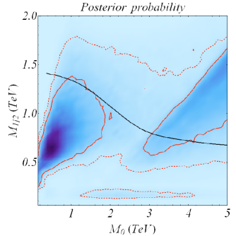
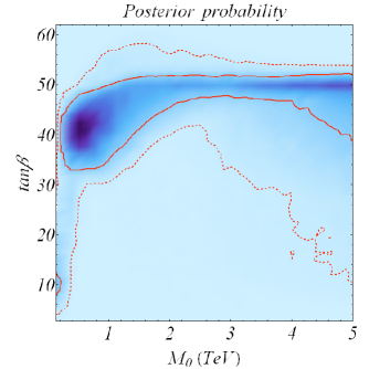
Figure 1: Posterior probabilities marginalized to pairs of NmSuGra input parameters. The higher probability regions are darker. Solid (dotted) red lines indicate 68 (95) percent confidence level contours. On the left frame the black curve shows the estimated reach of the LHC for 100 fb^-1 luminosity Baer:2003wx .

The top right frame of Figure 1 shows the distribution of the posterior probability in the $M_{0}$ vs. $\tan\beta$ frame. This makes it clear that most of the probable points are carried by Higgs resonant corridors toward higher $\tan\beta$, and the sfermion co-annihilation, due to its narrowness in $M_{0}$, falls only in the 95 % confidence, but is outside the 68 % region. The exception is a minute corner of the parameter space at very low $M_{0}$, $M_{1/2}$, and $\tan\beta\sim 10$ where all theoretical results conspire to match experiment, raising the sfermion co-annihilation region into the 68 % confidence region. At the opposite, high $M_{0}$ and $\tan\beta$ corner multiple Higgs resonances combined with neutralino-chargino co-annihilation in the focus point lead to substantial contribution to the total probability. A similar plot shows that positive values of $A_{0}$ are preferred over negative ones, because Higgs resonance annihilation occurs overwhelmingly at low to moderately positive values of $A_{0}$, and that $\lambda$ has little impact on the posterior.

0.5 Experimental detection of NmSuGra

We examine prospects of NmSuGra being detected at the LHC by plotting the posterior probability marginalized to the masses of relevant sparticles in Figure 2. Here we see that part of the NmSuGra parameter space, specifically the focus point, is out of the reach of the LHC, as shown by the posterior probability distribution of the gluino mass. In the mSuGra model the LHC is able to reach about 3 TeV gluinos with 100 fb^-1 luminosity, provided the model has low $M_{0}$ Baer:2003wx . In the focus point this reach is reduced to about 1.75 TeV.

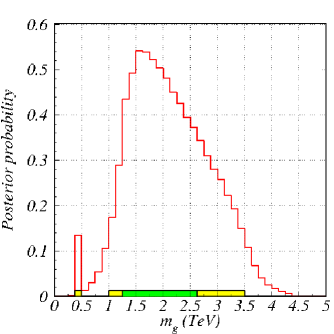
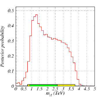
Figure 2: Posterior probability densities marginalized to gluino and stop masses.

In the lower left frame of Figure 2 shows that the lighter stop is also expected to be heavier than the likelihood alone would suggest. Even the sharp peak at low values in the stop likelihood function is overwhelmed due to the minute volume of the parameter space it occupies.

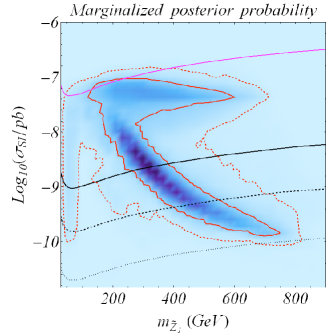
Figure 3: Posterior probability density marginalized to the spin-independent neutralino-nucleon elastic recoil cross section and the lightest neutralino mass. Confidence level contours are shown for 68 (solid red) and 95 (dashed red) %. The present (solid magenta) and projected reach of the upgraded CDMS experiment is shown for a 25 (solid black), 100 (dashed black), and a 1000 (dotted black) kg detector.

While the LHC will not be able to cover the full viable NmSuGra parameter space, fortunately a large part of the remaining region will be accessible to direct detection, measuring the spin-independent neutralino-nucleon elastic recoil cross section, $\sigma_{SI}$. From several of these experiments, we single out CDMS as the most illustrative example. Figure 3 shows the posterior probability density marginalized to the plane of $\sigma_{SI}$ and the lightest neutralino mass.

This plot clearly shows that direct detection experiments can play a pivotal role in discovering or ruling out simple constrained supersymmetric scenarios. Even a 25 kg CDMS will reach a substantial part of the focus point region, complementing the LHC.

In the possession of the above results, we can quantify the chances for the discovery of NmSuGra at the LHC by calculating the ratio of posterior probabilities inside and outside the reach of the LHC:

$$\frac{\int_{\rm within~{}LHC~{}reach}\mathcal{P}(p_{i}|D;H)dp_{i}}{\int_{\rm outside~{}LHC~{}reach}\mathcal{P}(p_{i}|D;H)dp_{i}}=0.57.$$ (5)

According to this the odds of finding NmSuGra at the LHC are 4:3 (assuming, of course, that the model is chosen by Nature). If we then include the reach of a ton equivalent of CDMS (CDMS1T), the NmSuGra model lies within the combined reach of the LHC and CDMS1T at 99 percent confidence level. This result strongly underlines the complementarity of collider and direct dark matter searches.

0.6 Conclusions

The next-to-minimal supergravity motivated model is one of the more compelling models for physics beyond the standard model due to its naturalness and simplicity. In this work we applied a thorough statistical analysis to NmSuGra based on numerical comparisons with present experimental data. Using Bayesian inference we find that the LHC and future CDMS limits cover the viable NmSuGra parameter region at 99 % confidence level, underlining the complementarity of these approaches to discovering new physics at the TeV scale. Thanks to the similarity between our model and the CMSSM, we expect these conclusions to be broadly valid in that model as well. However, this poses a challenge to the LHC experimentalists to disentangle these models.

The Multiple Point Principle: Characterization of the Possible Phases for the SMG D. L. Bennettdlbennett99@gmail.com

0.7 Introduction

The Multiple Point Principle (MPP) abel ; nonabel states that Nature takes on intensive parameter values (coupling constant values) that correspond to a maximally degenerate vacuum where these degenerate vacua all have essentially vanishing cosmological constants. The MPP was originally applied in the context of lattice gauge theory for the purpose of predicting the values of the three gauge coupling constants for the Standard Model Group (SMG). This pursuit entailed among other things a way in which to characterize the possible phases of of a non-simple gauge group such as the SMG. Having such a phase classification scheme, it was subsequently necessary to parameterize the action in such a way that these various phases could be provoked. In such an action parameter space our claim is that Nature takes on parameter values corresponding to the the point (or surface) — the multiple point — at which a maximum number phases come together.

The presentation at the 12th International Workshop “What Comes Beyond the Standard Model” in Bled (2009) was an attempt at a somewhat comprehensive review of the original implementation of the MPP. I was very happy that my talks were interrupted by so many questions. Many of these were about the formal way that different possible phases of the SMG are distinguished. So rather than a review of MPP I shall in this proceedings contribution address the questions posed. These were centered around the way in which the various possible phases for a non-simple gauge group such as the SMG are characterized in terms of subgroups $K\subseteq SMG$ and invariant subgroups $H\triangleleft K$. It will be seen that the subgroups $K$ and $H$ are defined according to the way that they transform under gauge transformations $\Lambda_{Const}$ and $\Lambda_{Linear}$ having respectively constant and linear gauge functions. The quantum fluctuation patterns characteristic of a given phase are defined in terms of $K\subseteq SMG$ and $H\triangleleft K$. We are working with a lattice formulation of a gauge theory. The different phases in such a theory are generally regarded as lattice artefacts. However we assume that a lattice is just one implementation of a fundamental really existing Planck scale regulator. In light of this assumption “lattice artefact” phases become ontological. That transitions between such phases are most often first order plays an important role in the finetunning mechanism inherent to MPP.

0.8 Distinguishing the possible phases of a non-simple group

Using a lattice formulation of a gauge theory with gauge group $G$, let the dynamics of the system be described by a Lagrangian ${\cal L}(A^{\mu},\phi)$ that is invariant under (local) gauge transformations $\Lambda$ of the gauge potential $A^{\mu}(x)$ and the (complex) scalar field $\phi(x)$. In the continuum, the fields $A^{\mu}(x)$ and $\phi(x)$ transform under gauge transformations as

$$gA^{\mu}(x)\rightarrow\Lambda^{-1}(x)gA^{\mu}(x)\Lambda(x)-i\Lambda^{-1}(x)\partial^{\mu}\Lambda(x)\;\;\;(\mbox{$g=$ coupling constant})$$ (6)

$$\phi(x)\rightarrow\Lambda(x)\phi(x)$$ (7)

In the lattice formulation, each of the four components of the $A^{\mu}$ field corresponds to a group-valued variable $U(\;\mbox{\begin{picture}(4.15,10.0)\put(0.0,3.0){\circle*{2.0}} \put(0.0,2.75){\line(1,0){7.0}} \put(7.3,3.0){\circle*{2.0}}\mbox{ } \end{picture} }^{\!\!\!\!\!\!\!x\;\;x+a\delta_{\nu}})$ defined on links of the lattice. The index $\nu$ specifies the direction of the link connecting sites with coordinates $x^{\rho}$ and $x^{\rho}+a\delta^{\rho}_{\nu}$; often such coordinates are written more briefly as $x$ and $x+a\delta_{\nu}$. Under a local gauge transformation, the $U(\;\mbox{\begin{picture}(4.15,10.0)\put(0.0,3.0){\circle*{2.0}} \put(0.0,2.75){\line(1,0){7.0}} \put(7.3,3.0){\circle*{2.0}}\mbox{ } \end{picture} }^{\!\!\!\!\!\!\!x\;\;x+a\delta_{\nu}})$ transform as

$$U(\;\mbox{\begin{picture}(4.15,10.0)\put(0.0,3.0){\circle*{2.0}} \put(0.0,2.75){\line(1,0){7.0}} \put(7.3,3.0){\circle*{2.0}}\mbox{ } \end{picture} }^{\!\!\!\!\!\!\!x\;\;x+a\delta_{\nu}})\rightarrow \Lambda^{-1}(x)U(\;\mbox{\begin{picture}(4.15,10.0)\put(0.0,3.0){\circle*{2.0}} \put(0.0,2.75){\line(1,0){7.0}} \put(7.3,3.0){\circle*{2.0}}\mbox{ } \end{picture} }^{\!\!\!\!\!\!\!x\;\;x+a\delta_{\nu}})\Lambda(x+a\delta_{\nu})\approx$$

$$\approx\Lambda^{-1}(x)U(\;\mbox{\begin{picture}(4.15,10.0)\put(0.0,3.0){\circle*{2.0}} \put(0.0,2.75){\line(1,0){7.0}} \put(7.3,3.0){\circle*{2.0}}\mbox{ } \end{picture} }^{\!\!\!\!\!\!\!x\;\;x+a\delta_{\nu}})(\Lambda(x)+\partial^{\rho}\Lambda(x)a\delta^{\rho}_{\nu})$$ (8)

$$=\Lambda^{-1}(x)U(\;\mbox{\begin{picture}(4.15,10.0)\put(0.0,3.0){\circle*{2.0}} \put(0.0,2.75){\line(1,0){7.0}} \put(7.3,3.0){\circle*{2.0}}\mbox{ } \end{picture} }^{\!\!\!\!\!\!\!x\;\;x+a\delta_{\nu}})\Lambda(x)(1+\partial^{\rho}(\log\Lambda(x))a\delta^{\rho}_{\nu})\approx$$

$$\approx\Lambda^{-1}(x)U(\;\mbox{\begin{picture}(4.15,10.0)\put(0.0,3.0){\circle*{2.0}} \put(0.0,2.75){\line(1,0){7.0}} \put(7.3,3.0){\circle*{2.0}}\mbox{ } \end{picture} }^{\!\!\!\!\!\!\!x^{\mu}\;\;y^{\mu}})\Lambda(x)\exp(\partial^{\rho}(\log\Lambda(x))a\delta^{\rho}_{\nu})$$

That this corresponds to the transformation (6) for the continuum fields $A^{\rho}$ is readily verified: write $U(\;\mbox{\begin{picture}(4.15,10.0)\put(0.0,3.0){\circle*{2.0}} \put(0.0,2.75){\line(1,0){7.0}} \put(7.3,3.0){\circle*{2.0}}\mbox{ } \end{picture} }^{\!\!\!\!\!\!\!x\;\;x+a\delta_{\nu}})=\exp(igA^{\rho}(x)a\delta_{\rho}^{\nu})\approx 1+igA^{\rho}(x)a\delta_{\rho}^{\nu}$ in which case the gauge transformation above is

$$\Lambda^{-1}(x)(1+igA^{\rho}(x)a\delta^{\nu}_{\rho})\Lambda(x)(1+\partial^{\rho}(\log\Lambda(x))a\delta^{\nu}_{\rho})\approx$$

$$\approx 1+\Lambda^{-1}(x)(igA^{\rho}(x)a\delta^{\nu}_{\rho})\Lambda(x)+\partial^{\rho}(\log\Lambda(x))a\delta^{\nu}_{\rho}=$$

$$=1+\Lambda^{-1}(x)(igA^{\rho}(x)a\delta^{\nu}_{\rho})\Lambda(x)+\Lambda^{-1}(x)\Lambda(x)\frac{1}{\Lambda(x)}\partial^{\rho}(\Lambda(x))a\delta^{\nu}_{\rho}$$

$$=1+i[\Lambda^{-1}(x)gA^{\rho}(x)\Lambda(x)-i\Lambda^{-1}(x)\partial^{\rho}(\Lambda(x))]a\delta^{\nu}_{\rho}$$

which corresponds to the transformation rule (6). On the lattice, the group-valued field $\phi$ is defined on lattice sites; the transformation rule is as in (7) above.

0.8.1 “Phase” classification according to symmetry properties of vacuum

We are interested in the case in which the gauge field $U(\;\mbox{\begin{picture}(4.15,10.0)\put(0.0,3.0){\circle*{2.0}} \put(0.0,2.75){\line(1,0){7.0}} \put(7.3,3.0){\circle*{2.0}}\mbox{ } \end{picture} }^{\!\!\!\!\!\!\!x\;\;x+a\delta_{\nu}})$ takes values in a non-simple gauge group such as $G=SMG$. The gauge field for the SMG has 12 degrees of freedom: if we allow a slight simplification one can say that 8 of these are associated with $SU(3)$ degrees of freedom, 3 with $SU(2)$ degrees of freedom   and one with the $U(1)$ degree of freedom.  It is possible for these degrees of freedom to take values in various structures all of which are determined for each choice $(K,H)$ such that $K\subseteq SMG$ and $H\triangleleft K$. The various structures are the subgroup $K$, the invariant subgroup $H$, the homogeneous space $SMG/K$ and the factor group $K/H$. For gauge field degrees of freedom there is a correspondence between distributions that characterize qualitatively different physical behaviors (e.g., quantum fluctuation patterns) and which structures the gauge field degrees of freedom take values in (e.g., elements of $K\subseteq G$ and $H\triangleleft K$ and cosets of $G/K$ and $K/H$. As already hinted, there is a one-to-one correspondence between the possible phases for the gauge field theory and the possible combinations $(K,H)$ with $K\subseteq G$ and $H\triangleleft K$. Discrete subgroups must be included among the possible subgroups. The choice of the pair $(K,H)$ specifies which degrees of freedom are in a Higgsed phase and also whether the un-Higgsed degrees of freedom are in a confined or Coulomb-like phase. Now I need to reveal how $K\subseteq G$ and $H\triangleleft K$ are defined.

The subgroups $K\subseteq G$ and $H\triangleleft K$ are defined by the transformation properties of the vacuum according to whether or not there is spontaneous breakdown of gauge symmetry under gauge transformations corresponding to the sets of gauge functions $\Lambda_{Const}$ and $\Lambda_{Linear}$ that are respectively constant and linear in the spacetime coordinatesfrogniel ; nonabel :

$$\Lambda_{Const}\in\{\Lambda:\mbox{\bf{R}}^{4}\rightarrow G|\exists\alpha[\forall x\in\mbox{\bf{R}}^{4}[\Lambda(x)=e^{i\alpha}]]\}$$ (9)

and

$$\Lambda_{Linear}\in\{\Lambda:\mbox{\bf{R}}^{4}\rightarrow G|\exists\alpha_{\mu}[\forall x\in\mbox{\bf{R}}^{4}[\Lambda(x)=e^{i\alpha_{\mu}x^{\mu}}]]\}.$$ (10)

Here $\alpha=\alpha^{a}t^{a}$ and $\alpha_{\mu}=\alpha^{a}_{\mu}t^{a}$ where $a$ labels the Lie algebra generators in the case of non-Abelian subgroups. The $t^{a}$ denote a basis of the Lie algebra satisfying the commutation relations $[t^{a},t^{b}]=c^{ab}_{c}t^{c}$ where the $c^{ab}_{c}$ are the structure constants.

Spontaneous symmetry breakdown is manifested as non-vanishing values for gauge variant quantities. However, according to Elitzur’s theorem, such quantities cannot survive under the full gauge symmetry. Hence a partial fixing of the gauge is necessary before it makes sense to talk about the spontaneous breaking of symmetry. We choose the Lorentz gauge for the reason that this still allows the freedom of making gauge transformations of the types $\Lambda_{Const}$ and $\Lambda_{Linear}$ to be used in classifying the lattice artifact “phases” of the vacuum. On the lattice, the choice of the Lorentz gauge amounts to the condition $\prod_{\;\;\mbox{\begin{picture}(4.15,10.0)\put(0.0,3.0){\circle*{2.0}} \put(0.0,2.75){\line(1,0){7.0}} \put(7.3,3.0){\circle*{2.0}}\mbox{ } \end{picture} }^{\!\!\!\!\!\!\!x^{\mu}\;\;}\;\tiny\mbox{emanating from }\mbox{\begin{picture}(4.15,4.0)\put(2.0,2.0){\circle*{2.0}} \end{picture} }^{\!\!\!x^{\mu}}}U(\mbox{\begin{picture}(4.15,10.0)\put(0.0,3.0){\circle*{2.0}} \put(0.0,2.75){\line(1,0){7.0}} \put(7.3,3.0){\circle*{2.0}}\mbox{ } \end{picture} })=1$ for all sites $\mbox{\begin{picture}(4.15,4.0)\put(2.0,2.0){\circle*{2.0}} \end{picture} }^{\!\!\!x}$.

By definition the degrees of freedom belonging to the subgroup $K$ exhaust the un-Higgsed degrees of freedom if, after fixing the gauge in accord with say the Lorentz condition, $K\subseteq G$ is the maximal subgroup of gauge transformations belonging to the set $\Lambda_{Const}$ that leaves the vacuum invariant For the vacuum of field variables defined on sites (denoted by $\langle\phi(\mbox{\begin{picture}(4.15,4.0)\put(2.0,2.0){\circle*{2.0}} \end{picture} }^{\!\!\!x^{\mu}})\rangle$), invariance under transformations $\Lambda_{Const.}$ is possible only if $\langle\phi(\mbox{\begin{picture}(4.15,4.0)\put(2.0,2.0){\circle*{2.0}} \end{picture} }^{\!\!\!x^{\mu}})\rangle=0$. For the vacuum of field variables defined on links (denoted by $\langle U(\;\mbox{\begin{picture}(4.15,10.0)\put(0.0,3.0){\circle*{2.0}} \put(0.0,2.75){\line(1,0){7.0}} \put(7.3,3.0){\circle*{2.0}}\mbox{ } \end{picture} }^{\!\!\!\!\!\!\!x\;\;x+a\delta_{\nu}})\rangle$, invariance under transformations $\Lambda_{Const}$ requires that $\langle U(\;\mbox{\begin{picture}(4.15,10.0)\put(0.0,3.0){\circle*{2.0}} \put(0.0,2.75){\line(1,0){7.0}} \put(7.3,3.0){\circle*{2.0}}\mbox{ } \end{picture} }^{\!\!\!\!\!\!\!x\;\;x+a\delta_{\nu}})\rangle$ takes values in the centre of the subgroup $K$. Conventionally, the idea of Higgsed degrees of freedom pertains to field variables defined on sites. With the above criterion using $\Lambda_{Const}$, the notion of Higgsed degrees of freedom is generalised to also include link variables.

If $K\subseteq G$ is the maximal subgroup for which the transformations $\Lambda_{Const}$ leave the vacuum invariant, the gauge field variables taking values in the homogeneous space $G/K$ (see for example dubrovin ; nakahara ) are by definition Higgsed in the vacuum. For these degrees of freedom, gauge symmetry is spontaneously broken in the vacuum under gauge transformations $\Lambda_{Const}$ (i.e., global gauge transformations).

In the vacuum, the un-Higgsed degrees of freedom - taking values in the subgroup $K$ - can be in a confining phase or a Coulomb-like phase according to the way these degrees of freedom transform under gauge transformations $\Lambda_{Linear}$ having linear gauge functions.

Degrees of freedom taking values in the invariant subgroup $H\triangleleft K$ are by definition confined in the vacuum if $H$ is the maximal invariant subgroup of gauge transformations $\Lambda_{Linear}$ that leaves the vacuum invariant; i.e., $h$ consists of the set of elements $h=\exp\{i\alpha^{1}_{a}t_{a}\}$ such that the gauge transformations with linear gauge function $\Lambda_{Linear}$ exemplified by$\Lambda_{Linear}\stackrel{{\scriptstyle def.}}{{=}}h^{x^{1}/a}$ leave the vacuum invariant.

If $H\triangleleft K$ is the maximal invariant subgroup of degrees of freedom that are confined in the vacuum, degrees of freedom taking as values the cosets belonging to the factor group $K/H$ are by definition in a Coulomb phase (again, in the Lorentz gauge). For degrees of freedom corresponding to this set of cosets, there is invariance of the vacuum expectation value under coset representatives of the type $\Lambda_{Const}$ while gauge symmetry is spontaneously broken in the vacuum under coset representatives of the type $\Lambda_{Linear}$.

Having now formal criteria for distinguishing the different phases of the vacuum, it would be useful to elaborate a bit further on what is meant by having a phase associated with a subgroup - invariant subgroup pair $(K_{i}\subseteq G,H_{j}\lhd K_{i})$. A phase is a characteristic region of action parameter space. Where does an action parameter space come from and what makes a region of it characteristic of a given phase $(K_{i}\subseteq G,H_{j}\lhd K_{i})$? An action parameter space comes about by choosing a functional form of the plaquette action. This will normally be a sum of terms each of which is a product of an action parameter (action parameters are related to coupling constants) multiplied by a sum over lattice plaquettes each term of which is the trace of group-valued plaquette variable in one of the desired representations (e.g., the fundamental representation, the adjoint representation, etc.).

Having an action allows the calculation of the partition function and subsequently the free energy. As each phase $(K_{i}\subseteq G,H_{j}\lhd K_{i})$ corresponds to different micro physical patterns of fluctuations along various group structures and homogeneous spaces as described above, the partition function and hence the free energy is a different function of the plaquette action parameters for each phase $(K_{i}\subseteq G,H_{j}\lhd K_{i})$. Have in mind that transitions between these “lattice artefact” phase are first order. A region of plaquette action parameter space is in a given phase $(K_{i}\subseteq G,H_{j}\lhd K_{i})$ if the free energy $-\log Z_{K_{i}\subseteq G,H_{j}\triangleleft K_{i}}$ associated with this phase has the largest value of all free energy functions. One should imagine that at any given point in the action parameter space all free energy funcions (one for each possible phase $(K,H)$) are defined (and have values). The realized phase at the point in question is determined by which of these free energy functions is the largest.

In seeking the multiple point, we seek the point or surface in parameter space where “all” (or a maximum number of) phases $(K_{i}\subseteq G,H_{j}\lhd K_{i})$ “touch” one another. MPP claims that action parameter values (which are simply related to coupling constants) at the multiple point are those realized in Nature.

0.9 The Higgsed phase

On a lattice consisting of sites $(\mbox{\begin{picture}(4.15,4.0)\put(2.0,2.0){\circle*{2.0}} \end{picture} }^{\!\!\!x^{\mu}})$ and site-connecting links $(\;\mbox{\begin{picture}(4.15,10.0)\put(0.0,3.0){\circle*{2.0}} \put(0.0,2.75){\line(1,0){7.0}} \put(7.3,3.0){\circle*{2.0}}\mbox{ } \end{picture} }^{\!\!\!\!\!\!\!x^{\mu}\;\;y^{\mu}})$ denote by $\phi(\mbox{\begin{picture}(4.15,4.0)\put(2.0,2.0){\circle*{2.0}} \end{picture} }^{\!\!\!x^{\mu}})$ a scaler field variable defined on lattice sites. We want to describe the conditions to be fulfilled if the field variable $\phi(\mbox{\begin{picture}(4.15,4.0)\put(2.0,2.0){\circle*{2.0}} \end{picture} }^{\!\!\!x^{\mu}})$ is a Higgsed degree of freedom. The appropriate mathematical structure is that of a homogeneous space. If $K\subseteq SMG$ ($K$ not an invariant subgroup of SMG) is the subgroup of not-Higgsed gauge degrees of freedom, the Higgsed degrees of freedom $\phi(\mbox{\begin{picture}(4.15,4.0)\put(2.0,2.0){\circle*{2.0}} \end{picture} }^{\!\!\!x^{\mu}})$ take values in the homogeneous space $SMG/K$

It might be be useful with a reminder about the mathematical structure of a homogeneous space. For the purpose of exposition it is expedient to use the example of the group $G=SO(3)$ instead of the $G=SMG$ and the subgroup $SO(2)\subset SO(3)$ (instead of the unspecified $K\subseteq SMG$). So we consider the homogeneous space $SO(3)/SO(2)$. In this case the cosets (i.e. elements) of $SO(3)/SO(2)$ are in one-to-one correspondence with the points on a $S_{2}$ sphere: for an arbitrary coset $h\in SO(3)/SO(2)$, the orbit of the action of $SO(3)$ on $h$ is just $S_{2}$. The homogeneous space $SO(3)/SO(2)$ is mapped onto itself under the action of $SO(3)$:

$$h_{2}\stackrel{{\scriptstyle g\in SO(3)}}{{\longrightarrow}}h_{1}\;\;\;(h_{1},h_{2}\in SO(3)/SO(2);$$

Note that there is no multiplication (i.e., composition) rule for the cosets (i.e., elements) of a homogeneous space. For example, $h_{1}\cdot h_{2}$ for $h_{1},h_{2}\in SO(3)/SO(2)$ is not meaningful. It can be shown that the action the group $G$ on the homogeneous space $G/K$ is transitive which means that for any two cosets $h_{1},h_{2}\in G/K$ there exists at least one element $g\in G$ such that $h_{1}=gh_{2}$. In the example with $G=SO(3)$ and $G/K=SO(3)/SO(2)$ this means that for any two points $h_{1}$ and $h_{2}$ on $S_{2}\cong SO(3)/SO(2)$ there is at least one element $g\in SO(3)$ such that $h_{1}=gh_{2}$. The set of such elements $g$:

$$\{g\in SO(3)|gh_{2}=h_{1}\}$$

is the coset of $SO(3)/SO(2)$ associated with $h_{1}$ (here $h_{2}$ can be thought of as a (arbitrarily chosen) basis coset from which all other cosets of $SO(3)/SO(2)$ can be obtained by the appropriate action of $SO(3)$).

Any element $g^{\prime}$ belonging to the coset $\{g\in SO(3)|gh_{2}=h_{1}\}$ is a representative of this coset associated with $h_{1}$. Other representatives of this same coset are obtained by letting $g^{\prime}$ act on the $SO(2)\subset SO(3)$ that leaves the basis coset $h_{2}$ invariant (denote the latter by $SO(2)_{h_{2}\,inv}$). In fact all of the representatives of the coset $\{g\in SO(3)|gh_{2}=h_{1}\}$ are given by $g^{\prime}\cdot SO(2)_{h_{2}\,inv}$. So when $g^{\prime}$ is a representative of the coset associated with $h_{1}$, so is $g^{\prime}\cdot k$ when $k\in SO(2)_{h_{2}\,inv}$. It goes without saying that a representative of a coset always belongs to the coset that it represents.

To get a feeling for it means to have a Higgsed phase, think of having an $S_{2}$ situated at each site $\mbox{\begin{picture}(4.15,4.0)\put(2.0,2.0){\circle*{2.0}} \end{picture} }^{\!\!\!x^{\mu}}$ of the (space-time) lattice. In this picture, the variable $\phi(\mbox{\begin{picture}(4.15,4.0)\put(2.0,2.0){\circle*{2.0}} \end{picture} }^{\!\!\!x^{\mu}})$ at each site $\mbox{\begin{picture}(4.15,4.0)\put(2.0,2.0){\circle*{2.0}} \end{picture} }^{\!\!\!x^{\mu}}$ corresponds to a point on the $S_{2}$ at this site. A priori there is no special point in this homogeneous space $SO(3)/SO(2)\stackrel{{\scriptstyle-}}{{\simeq}}S_{2}$ which implies $\langle\phi(\mbox{\begin{picture}(4.15,4.0)\put(2.0,2.0){\circle*{2.0}} \end{picture} })\rangle=0$. The Higgs mechanism comes into play when, for all sites on the lattice, the vacuum value of $\phi(\mbox{\begin{picture}(4.15,4.0)\put(2.0,2.0){\circle*{2.0}} \end{picture} })$ - modulo parallel transport between sites by link variables - is (in a classical approximation) the same coset of $SO(3)/SO(2)$ or in other words the same point on all the (site situated) $S_{2}$’s (modulo parallel transport) inasmuch as $SO(3)/SO(2)\cong S_{2}$. With one point of $S_{2}$ singled out globally - call it $h_{2}$ - it is obvious that $\langle\phi(\mbox{\begin{picture}(4.15,4.0)\put(2.0,2.0){\circle*{2.0}} \end{picture} })\rangle\neq 0$. The symmetry of the homogeneous space $SO(3)/SO(2)$ is broken globally down to the $SO(2)\subset SO(3)$ that leaves the point $h_{2}\in S_{2}$ invariant. This is just the isotropy group of $h_{2}\in S_{2}$ which we can - using a notation defined above - denote as $SO(2)_{h_{2}\>inv.}$. After a Higgsning corresponding to singling out $h_{2}\in S_{2}$ we can think of $h_{2}$ as the axis about which the symmetry remaining after this Higgsning are just the rotations $SO(2)_{h_{2}\>inv.}$.

In a quantum field theoretic description of a Higgsed phase corresponding to $h_{2}\in S_{2}$ where we allow for quantum fluctuations, we expect a clustering of the values of $\phi(\mbox{\begin{picture}(4.15,4.0)\put(2.0,2.0){\circle*{2.0}} \end{picture} })$ about the coset $h_{2}\in S_{2}$ for all sites of the lattice (modulo parallel transport). This brings us to a technical problemhbnpriv : the average value of such quantum fluctuations is expected to be $h_{2}$: $\langle\phi(\mbox{\begin{picture}(4.15,4.0)\put(2.0,2.0){\circle*{2.0}} \end{picture} })\rangle=h_{2}$. But the average value of for example two cosets of in the neighborhood of the coset corresponding $h_{2}$ does not lie in $S_{2}\cong SO(3)/SO(2)$ but rather in the interior of $S_{2}$ (the convex closure). In order to have such average values in our target space we need the convex closure of $S_{2}$.

The Higgs mechanism outlined above can be provoked if there is a term in the action of the form

$$\kappa dist^{2}(\phi(\mbox{\begin{picture}(4.15,4.0)\put(2.0,2.0){\circle*{2.0}} \end{picture} }^{\!\!\!x}),U(\;\mbox{\begin{picture}(4.15,10.0)\put(0.0,3.0){\circle*{2.0}} \put(0.0,2.75){\line(1,0){7.0}} \put(7.3,3.0){\circle*{2.0}}\mbox{ } \end{picture} }^{\!\!\!\!\!\!\!x\;\;y})\phi(\mbox{\begin{picture}(4.15,4.0)\put(2.0,2.0){\circle*{2.0}} \end{picture} }^{\!\!\!\!\!y}))$$ (11)

where $\kappa$ is a parameter and $dist^{2}(\phi(\mbox{\begin{picture}(4.15,4.0)\put(2.0,2.0){\circle*{2.0}} \end{picture} }^{\!\!\!x}),U(\;\mbox{\begin{picture}(4.15,10.0)\put(0.0,3.0){\circle*{2.0}} \put(0.0,2.75){\line(1,0){7.0}} \put(7.3,3.0){\circle*{2.0}}\mbox{ } \end{picture} }^{\!\!\!\!\!\!\!x\;\;y})\phi(\mbox{\begin{picture}(4.15,4.0)\put(2.0,2.0){\circle*{2.0}} \end{picture} }^{\!\!\!\!\!y}))$ is the suitably defined squared distance on the $S_{2}$ at the site $\mbox{\begin{picture}(4.15,4.0)\put(2.0,2.0){\circle*{2.0}} \end{picture} }^{\!\!\!x}$ between the point $\phi(\mbox{\begin{picture}(4.15,4.0)\put(2.0,2.0){\circle*{2.0}} \end{picture} }^{\!\!\!x})$ and the point $\phi(\mbox{\begin{picture}(4.15,4.0)\put(2.0,2.0){\circle*{2.0}} \end{picture} }^{\!\!\!\!\!y})$ after the latter is “parallel transported” to $\mbox{\begin{picture}(4.15,4.0)\put(2.0,2.0){\circle*{2.0}} \end{picture} }^{\!\!\!x}$ using the link variable $U(\;\mbox{\begin{picture}(4.15,10.0)\put(0.0,3.0){\circle*{2.0}} \put(0.0,2.75){\line(1,0){7.0}} \put(7.3,3.0){\circle*{2.0}}\mbox{ } \end{picture} }^{\!\!\!\!\!\!\!x\;\;y})\in G$. This is the so-called Manton actionmanton .

In terms of of elements $g\in SO(3)$,

$$dist^{2}(\phi(\mbox{\begin{picture}(4.15,4.0)\put(2.0,2.0){\circle*{2.0}} \end{picture} }^{\!\!\!x}),U(\;\mbox{\begin{picture}(4.15,10.0)\put(0.0,3.0){\circle*{2.0}} \put(0.0,2.75){\line(1,0){7.0}} \put(7.3,3.0){\circle*{2.0}}\mbox{ } \end{picture} }^{\!\!\!\!\!\!\!x\;\;y})\phi(\mbox{\begin{picture}(4.15,4.0)\put(2.0,2.0){\circle*{2.0}} \end{picture} }^{\!\!\!\!\!y}))\stackrel{{\scriptstyle def}}{{=}}$$ (12)

$$inf\{dist^{2}(g_{x}\cdot SO(2),U(\;\mbox{\begin{picture}(4.15,10.0)\put(0.0,3.0){\circle*{2.0}} \put(0.0,2.75){\line(1,0){7.0}} \put(7.3,3.0){\circle*{2.0}}\mbox{ } \end{picture} }^{\!\!\!\!\!\!\!x\;\;y})g_{y}\cdot SO(2)|$$

$$\mbox{ $g_{x}$ \& $g_{y}$ \footnotesize are reps. of respectively the cosets $\phi(\mbox{\begin{picture}(4.15,4.0)\put(2.0,2.0){\circle*{2.0}} \end{picture} }^{\!\!\!x})$ \& $\phi(\mbox{\begin{picture}(4.15,4.0)\put(2.0,2.0){\circle*{2.0}} \end{picture} }^{\!\!\!\!\!y})$}\}$$

In order to provoke the Higgs mechanism, not only must the parameter $\kappa$ be sufficiently large to ensure that it doesn’t pay not to have clustered values of the variables $\phi(\cdot)$. It is also necessary that “parallel transport” be well defined so that it makes sense to talk about the values of $\phi(\mbox{\begin{picture}(4.15,4.0)\put(2.0,2.0){\circle*{2.0}} \end{picture} })$ being organised (i.e., clustered) at some coset of $SO(3)/SO(2)$. This would obviously not be the case if the theory were confined. In confinement, $\langle U(\;\mbox{\begin{picture}(4.15,10.0)\put(0.0,3.0){\circle*{2.0}} \put(0.0,2.75){\line(1,0){7.0}} \put(7.3,3.0){\circle*{2.0}}\mbox{ } \end{picture} }^{\!\!\!\!\!\!\!x\;\;y})\rangle=0$ and parallel transport is meaningless. In the continuum theory, this would correspond to having large curvature (i.e., large $F_{\mu\nu}$) which in turn would make parallel transport very path dependent

0.10 The un-Higgsed Phases

The un-Higgsed gauge field degrees of freedom (i.e., link variables) take values that correspond to the Lie algebra of the subgroup $K\subseteq G$. The confined degrees of freedom take as values the elements of the invariant subgroup $H\triangleleft K$. The Coulomb-like degrees of freedom take as values the cosets of the factor group $K/H$.

0.10.1 Confined degrees of freedom

The confined phase is characterized by large quantum fluctuations in the group-valued link variables so that at least crudely speaking the whole confined subgroup $H$ is accessed. So roughly speaking all elements $h\in H$ are visited with nearly the same probability. In other words the distribution of quantum fluctuations for confined link variables is not strongly clustered in a small part of the group space (e.g. at the group identity or in the center of the group). Since the distribution of confined degrees of freedom is essentially flat (i.e., without much characteristic structure) the effect of gauge transformations is not noticeable. The subgroup $H$ is therefore essentially invariant under all classes of gauge transformations including the for us interesting types of gauge transformation $\Lambda_{Const}$ and $\Lambda_{Linear}$.

0.10.2 The Coulomb-like phase

The claim above is that Coulomb-like link variable degrees of freedom take as values the cosets of the factor group $K/H$. Recall that by definition of a factor group all of the elements of $H$ are identified (i.e., not distinguishable from one another) and the (invariant) subgroup $H$ becomes the identity element in the coset space. That elements of $H$ are not distinguished from one another is consistent with the intuitive properties of having confinement along the subgroup $H$ as sketched above: a consequence of having large quantum fluctuations along $H$ is that all elements of $H$ enter into the fluctuation pattern (which is a manifestation of the underlying physics) with essentially the same weight (as opposed to e.g., a Coulomb-like phase in which the fluctuation pattern is more or less tightly clustered around the group identity).

The transformation properties of the vacuum that are appropriate for having a Coulomb-like phase are suggested by examining the requirementsfrogniel for getting a massless gauge particle as the Nambu-Goldstone boson accompanying the spontaneous breakdown of gauge symmetry. To this end we need to examine the Goldstone Theorem

As already pointed out, a gauge choice must be made in order that spontaneous breakdown of gauge symmetry is at all possible. Otherwise Elitzur’s Theorem insures that all gauge variant quantities vanish identically. Once a gauge choice is made - the Lorenz gauge is strongly suggested inasmuch as we want, in order to classify phases, to retain the freedom to make gauge transformations of the types $\Lambda_{Const}$ and $\Lambda_{Linear}$ - the symmetry under the remaining gauge symmetry must somehow be broken in order to get a Nambu-Goldstone boson that, according to the Nambu-Goldstone Theorem, is present for each generator of a spontaneously broken continuous gauge symmetry.

Recalling from (8) that a link variable $U(\;\mbox{\begin{picture}(4.15,10.0)\put(0.0,3.0){\circle*{2.0}} \put(0.0,2.75){\line(1,0){7.0}} \put(7.3,3.0){\circle*{2.0}}\mbox{ } \end{picture} }^{\!\!\!\!\!\!\!x^{\mu}\;\;y^{\mu}})$ transforms under gauge transformations as

$$U(\;\mbox{\begin{picture}(4.15,10.0)\put(0.0,3.0){\circle*{2.0}} \put(0.0,2.75){\line(1,0){7.0}} \put(7.3,3.0){\circle*{2.0}}\mbox{ } \end{picture} }^{\!\!\!\!\!\!\!x\;\;x+a\delta_{\nu}})\rightarrow\Lambda^{-1}(x)U(\;\mbox{\begin{picture}(4.15,10.0)\put(0.0,3.0){\circle*{2.0}} \put(0.0,2.75){\line(1,0){7.0}} \put(7.3,3.0){\circle*{2.0}}\mbox{ } \end{picture} }^{\!\!\!\!\!\!\!x\;\;x+a\delta_{\nu}})\Lambda(x)\cdot\underbrace{\exp(\partial^{\rho}(\log\Lambda(x))\cdot a\delta^{\nu}_{\rho}}_{\mbox{\footnotesize gradient part of transf.}},$$ (13)

it is seen that, for the special case of an Abelian gauge group, a gauge function that is linear in the coordinates (or higher order in the coordinates) is required for spontaneous breakdown because the only possibility for spontaneously breaking the symmetry comes from the “gradient” part of the transformation (13). So the needed spontaneous breakdown of gauge symmetry is garanteed if gauge symmetry for gauge transformations of the type $\Lambda_{Linear}$ is spontaneously broken (i.e., the vacuum is not invariant under this class of gauge transformations). Let $Q_{\nu}$ denote the generator of such gauge transformations.

However the proof of the Nambu-Goldstone Theorem also requires the assumption of translational invariance. This amounts to the requirement that the vacuum be invariant under gauge transformations generated by the commutator of the momentum operator with the generator of the spontaneously broken symmetry which is just $Q_{\nu}$ as defined above. Then the requirement of translational symmetry is equivalent to requiring that the vacuum $\langle U(\;\mbox{\begin{picture}(4.15,10.0)\put(0.0,3.0){\circle*{2.0}} \put(0.0,2.75){\line(1,0){7.0}} \put(7.3,3.0){\circle*{2.0}}\mbox{ } \end{picture} }^{\!\!\!\!\!\!\!x\;\;x+a\delta_{\nu}})\rangle$ is annihilated by the commutator $[P_{\mu},Q_{\nu}]=ig_{\mu\nu}Q$ where $Q$ denotes the generator of gauge transformations with constant gauge functions. So the condition for having translational invariance translates into the requirement that the vacuum $\langle U(\;\mbox{\begin{picture}(4.15,10.0)\put(0.0,3.0){\circle*{2.0}} \put(0.0,2.75){\line(1,0){7.0}} \put(7.3,3.0){\circle*{2.0}}\mbox{ } \end{picture} }^{\!\!\!\!\!\!\!x\;\;x+a\delta_{\nu}})\rangle$ be invariant under gauge transformations with constant gauge functions. An examination of (13) verifies that this is always true for Abelian gauge groups and also for non-Abelian groups if the vacuum expectation value $\langle U(\;\mbox{\begin{picture}(4.15,10.0)\put(0.0,3.0){\circle*{2.0}} \put(0.0,2.75){\line(1,0){7.0}} \put(7.3,3.0){\circle*{2.0}}\mbox{ } \end{picture} }^{\!\!\!\!\!\!\!x\;\;x+a\delta_{\nu}})\rangle$ lies in the centre of the group (which just means that the vacuum is not “Higgsed”).

0.11 Summary and Concluding Remarks

We have presented a formalism that can be used to define the various possible phases for a non-simple gauge group in the context of lattice gauge theory (LGT). Specifically we are interested in the non-simple $SMG$. These phases are normally said to be artefacts of the unphysical lattice regulator. As we assume that a lattice is one way to implement what we take to be a fundamental ontological (roughly Planck scale) regulator, the “artefact” phases take on a physical meaning.

The various phases are realized by adjusting intensive parameters (which are closely related to the couplings) in the action. These span the so-called action parameter space which is the space in which the boundaries separating the various possible phases can be constructed in a way analogous to the way that temperature and pressure span the space in which the boundaries separating the solid, liquid and gaseous phases of $H_{2}O$ can be drawn. In LGT a typical term in the action is the product of such an intensive parameter with the trace in some representation of a gauge group element defined on a lattice plaquette. In each action term these traces are summed over the plaquettes of the lattice

In this contribution we have developed the formalism for distinguishing the possible phases of a non-simple gauge group $G$ each of which corresponds to a pair of subgroups $(K,H)$ such that $K\subseteq G$ and $H\triangleleft K$.

For each phase $(K,H)$ the free energy $-\log Z_{K_{i}\subseteq G,H_{j}\triangleleft K_{i}}$ is defined for the entire action parameter space. At any point in this space, the phase realized is that for the free enery function has the largest value.

The point in the action parameter space at which the maximum number of different phases come together - the multiple point - corresponds according to the MPP to the parameter values (couplings) realized in Nature. At this point the free energy functions for all the phases that come together at the multiple point are of course all equal.

The degrees of freedom belonging to the subgroup $K$ are the un-Higgsed degrees of freedom if, after fixing the gauge in accord with say the Lorentz condition, $K\subseteq G$ is the maximal subgroup of gauge transformations belonging to the set $\Lambda_{Const}$ that leaves the vacuum invariant. The field variables taking values in the homogeneous space $G/K$ are by definition Higgsed in the vacuum. For these degrees of freedom, gauge symmetry is spontaneously broken in the vacuum under global gauge transformations $\Lambda_{Const}$.

Degrees of freedom taking values in the invariant subgroup $H\triangleleft K$ are by definition confined in the vacuum if $H$ is the maximal invariant subgroup of gauge transformations $\Lambda_{Linear}$ that leaves the vacuum invariant.

The degrees of freedom in a Coulomb-like phase take as values the cosets of the factor group $K/H$. The symmetry properties of the vacuum for a Coulomb-like phase are dictated by the requirements of the Goldstone Theorem. The conditions to be fulfilled in order that the Nambu-Goldstone boson accompanying a spontaneous breakdown of gauge symmetry can be identified with a massless gauge particle (the existence of which is the characteristic feature of a Coulomb-like phase) suggests that the Coulomb phase vacuum is invariant under gauge transformations having a constant gauge function but spontaneously broken under gauge transformations having linear gauge functions.

Summarizing one can say that each phase corresponds to a partitioning of the degrees of freedom (these latter can be labelled by a Lie algebra basis) - some that are Higgsed, others that are un-Higgsed; of the latter, some degrees of freedom can be confining, others Coulomb-like. It is useful to think of a group element $U$ of the gauge group as being parameterized in terms of three sets of coordinates corresponding to three different structures that are appropriate to the symmetry properties used to define a given phase $(K,H)$ of the vacuum. These three sets of coordinates, which are definable in terms of the gauge group $G$, the subgroup $K$, and the invariant subgroup $H\triangleleft K$, are the homogeneous space $G/K$, the factor group $K/H$, and $H$ itself:

$$U=U(g,k,h)\;\;\mbox{with }\;g\in G/K,k\in K/H,h\in H.$$ (14)

The coordinates $g\in G/K$ will be seen to correspond to Higgsed degrees of freedom, the coordinates $k\in K/H$ to un-Higgsed, Coulomb-like degrees of freedom and the coordinates $h\in H$ to un-Higgsed, confined degrees of freedom.

Does Dark Matter Consist of Baryons of New Stable Family Quarks? G. Bregar and N.S. Mankoč Borštnik

0.12 Introduction

Although the origin of the dark matter is unknown, its gravitational interaction with the known matter and other cosmological observations require from the candidate for the dark matter constituent that: i. The scattering amplitude of a cluster of constituents with the ordinary matter and among the dark matter clusters themselves must be small enough, so that no effect of such scattering has been observed, except possibly in the DAMA/NaI gbsnmbrita0708 and not (yet?) in the CDMS and other experiments gbsnmbcdms . ii. Its density distribution (obviously different from the ordinary matter density distribution) causes that all the stars within a galaxy rotate approximately with the same velocity (suggesting that the density is approximately spherically symmetrically distributed, descending with the second power of the distance from the center, it is extended also far out of the galaxy, manifesting the gravitational lensing by galaxy clusters). iii. The dark matter constituents must be stable in comparison with the age of our universe, having obviously for many orders of magnitude different time scale for forming (if at all) solid matter than the ordinary matter. iv. The dark matter constituents had to be formed during the evolution of our universe so that they contribute today the main part of the matter ((5-7) times as much as the ordinary matter).

There are several candidates for the massive dark matter constituents in the literature, like, for example, WIMPs (weakly interacting massive particles), the references can be found in gbsnmbdodelson ; gbsnmbrita0708 . In this paper we discuss the possibility that the dark matter constituents are clusters of a stable (from the point of view of the age of the universe) family of quarks and leptons. Such a family is predicted by the approach unifying spin and charges gbsnmbpn06 ; gbsnmbn92 ; gbsnmbgmdn07 , proposed by one of the authors of this paper: N.S.M.B. This approach is showing a new way beyond the standard model of the electroweak and colour interactions by answering the open questions of this model like: Where do the families originate?, Why do only the left handed quarks and leptons carry the weak charge, while the right handed ones do not? Why do particles carry the observed $SU(2),U(1)$ and $SU(3)$ charges? Where does the Higgs field originate from?, and others.

There are several attempts in the literature trying to understand the origin of families. All of them, however, in one or another way (for example through choices of appropriate groups) simply postulate that there are at least three families, as does the standard model of the electroweak and colour interactions. Proposing the (right) mechanism for generating families is to our understanding the most promising guide to physics beyond the standard model.

The approach unifying spin and charges is offering the mechanism for the appearance of families. It introduces the second kind gbsnmbpn06 ; gbsnmbn92 ; gbsnmbn93 ; gbsnmbhn02hn03 of the Clifford algebra objects, which generates families as the equivalent representations to the Dirac spinor representation. The references gbsnmbn93 ; gbsnmbhn02hn03 show that there are two, only two, kinds of the Clifford algebra objects, one used by Dirac to describe the spin of fermions. The second kind forms the equivalent representations with respect to the Lorentz group for spinors gbsnmbpn06 and the families do form the equivalent representations with respect to the Lorentz group. The approach, in which fermions carry two kinds of spins (no charges), predicts from the simple starting action more than the observed three families. It predicts two times four families with masses several orders of magnitude bellow the unification scale of the three observed charges.

Since due to the approach (after assuming a particular, but to our opinion trustable, way of a nonperturbative breaking of the starting symmetry) the fifth family decouples in the Yukawa couplings from the lower four families (whose the fourth family quark’s mass is predicted to be at around $250$ GeV or above gbsnmbpn06 ; gbsnmbgmdn07 ), the fifth family quarks and leptons are stable as required by the condition iii.. Since the masses of all the members of the fifth family lie, due to the approach, much above the known three and the predicted fourth family masses, the baryons made out of the fifth family form small enough clusters (as we shall see in section 0.13) so that their scattering amplitude among themselves and with the ordinary matter is small enough and also the number of clusters (as we shall see in section 0.14) is low enough to fulfil the conditions i. and iii.. Our study of the behaviour of the fifth family quarks in the cosmological evolution (section 0.14) shows that also the condition iv. is fulfilled, if the fifth family masses are large enough.

Let us add that there are several assessments about masses of a possible (non stable) fourth family of quarks and leptons, which follow from the analyses of the existing experimental data and the cosmological observations. Although most of physicists have doubts about the existence of any more than the three observed families, the analyses clearly show that neither the experimental electroweak data gbsnmbokun ; gbsnmbpdg , nor the cosmological observations gbsnmbpdg forbid the existence of more than three families, as long as the masses of the fourth family quarks are higher than a few hundred GeV and the masses of the fourth family leptons above one hundred GeV ($\nu_{4}$ could be above $50$ GeV). We studied in the ¨references gbsnmbpn06 ; gbsnmbgmdn07 ; gbsnmbn09 possible (non perturbative) breaks of the symmetries of the simple starting Lagrangean which, by predicting the Yukawa couplings, leads at low energies first to twice four families with no Yukawa couplings between these two groups of families. One group obtains at the last break masses of several hundred TeV or higher, while the lower four families stay massless and mass protected gbsnmbn09 . For one choice of the next break gbsnmbgmdn07 the fourth family members ($u_{4},d_{4},\nu_{4},e_{4}$) obtain the masses at ($224$ GeV (285 GeV), $285$ GeV (224 GeV), $84$ GeV, $170$ GeV), respectively. For the other choice of the next break we could not determine the fourth family masses, but when assuming the values for these masses we predicted mixing matrices in dependence on the masses. All these studies were done on the tree level. We are studying now symmetries of the Yukawa couplings if we go beyond the tree level. Let us add that the last experimental data gbsnmbmoscow09 from the HERA experiments require that there is no $d_{4}$ quark with the mass lower than $250$ GeV.

Our stable fifth family baryons, which might form the dark matter, also do not contradict the so far observed experimental data—as it is the measured (first family) baryon number and its ratio to the photon energy density, as long as the fifth family quarks are heavy enough ($>1$ TeV). (This would be true for any stable heavy family.) Namely, all the measurements, which connect the baryon and the photon energy density, relate to the moment(s) in the history of the universe, when baryons of the first family where formed ($k_{b}T$ bellow the binding energy of the three first family quarks dressed into constituent mass of $m_{q_{1}}c^{2}\approx 300$ MeV, that is bellow $10$ MeV) and the electrons and nuclei formed atoms ($k_{b}\,T\approx 1$ eV). The chargeless (with respect to the colour and electromagnetic charges) clusters of the fifth family were formed long before (at $k_{b}T\approx E_{c_{5}}$ (see Table 1)), contributing the equal amount of the fifth family baryons and anti-baryons to the dark matter, provided that there is no fifth family baryon—anti-baryon asymmetry (if the asymmetry is nonzero the colourless baryons or anti-baryons are formed also at the early stage of the colour phase transition at around $1$ GeV). They manifest after decoupling from the plasma (with their small number density and small cross section) (almost) only their gravitational interaction.

In this paper we estimate the properties of the fifth family members ($u_{5}$, $d_{5}$, $\nu_{5}$, $e_{5}$), as well as of the clusters of these members, in particular the fifth family neutrons, under the assumptions that:
I. Neutron is the lightest fifth family baryon.
II. There is no fifth family baryon—anti-baryon asymmetry.
The assumptions are made since we are not yet able to derive the properties of the family from the starting Lagrange density of the approach. The results of the present paper’s study are helpful to better understand steps needed to come from the approach’s starting Lagrange density to the low energy effective one.

From the approach unifying spin and charges we learn:
i. The stable fifth family members have masses higher than $\approx 1$ TeV and smaller than $\approx 10^{6}$ TeV.
ii. The stable fifth family members have the properties of the lower four families; that is the same family members with the same (electromagnetic, weak and colour) charges and interacting correspondingly with the same gauge fields.

We estimate the masses of the fifth family quarks by studying their behaviour in the evolution of the universe, their formation of chargeless (with respect to the electromagnetic and colour interaction) clusters and the properties of these clusters when scattering on the ordinary (made mostly of the first family members) matter and among themselves. We use a simple (the hydrogen-like) model gbsnmbgnBled07 to estimate the size and the binding energy of the fifth family baryons, assuming that the fifth family quarks are heavy enough to interact mostly by exchanging one gluon. We solve the Boltzmann equations for the fifth family quarks (and anti-quarks) forming the colourless clusters in the expanding universe, starting in the energy region when the fifth family members are ultrarelativistic, up to $\approx 1$ GeV when the colour phase transition starts. In this energy interval the one gluon exchange is the dominant interaction among quarks and the plasma. We conclude that the quarks and anti-quarks, which succeed to form neutral (colourless and electromagnetic chargeless) clusters, have the properties of the dark matter constituents if their masses are within the interval of a few TeV $<m_{q_{5}}c^{2}<$ a few hundred TeV, while the rest of the coloured fifth family objects annihilate within the colour phase transition period with their anti-particles for the zero fifth family baryon number asymmetry.

We estimate also the behaviour of our fifth family clusters if hitting the DAMA/NaI—DAMA-LIBRA gbsnmbrita0708 and CDMS gbsnmbcdms experiments presenting the limitations the DAMA/NaI experiments put on our fifth family quarks when recognizing that CDMS has not found any event (yet).

The fifth family baryons are not the objects (WIMPS), which would interact with only the weak interaction, since their decoupling from the rest of the plasma in the expanding universe is determined by the colour force and their interaction with the ordinary matter is determined with the fifth family ”nuclear force” (this is the force among clusters of the fifth family quarks, manifesting much smaller cross section than does the ordinary, mostly first family, ”nuclear force”) as long as their mass is not higher than $10^{4}$ TeV, when the weak interaction starts to dominate as commented in the last paragraph of section 0.15.

0.13 Properties of clusters of the heavy family

Let us study the properties of the fifth family of quarks and leptons as predicted by the approach unifying spin and charges, with masses several orders of magnitude greater than those of the known three families, decoupled in the Yukawa couplings from the lower mass families and with the charges and their couplings to the gauge fields of the known families (which all seems, due to our estimate predictions of the approach, reasonable assumptions). Families distinguish among themselves (besides in masses) in the family index (in the quantum number, which in the approach is determined by the second kind of the Clifford algebra objects’ operators gbsnmbpn06 ; gbsnmbn92 ; gbsnmbn93 $\tilde{S}^{ab}=\frac{i}{4}(\tilde{\gamma}^{a}\tilde{\gamma}^{b}-\tilde{\gamma}^{b}\tilde{\gamma}^{a})$, anti-commuting with the Dirac $\gamma^{a}$’s), and (due to the Yukawa couplings) in their masses.

For a heavy enough family the properties of baryons (protons $p_{5}$ $(u_{5}u_{5}d_{5})$, neutrons $n_{5}$ $(u_{5}d_{5}d_{5})$, $\Delta_{5}^{-}$, $\Delta_{5}^{++}$) made out of quarks $u_{5}$ and $d_{5}$ can be estimated by using the non relativistic Bohr-like model with the $\frac{1}{r}$ dependence of the potential between a pair of quarks $V=-\frac{2}{3}\frac{\hbar c\,\alpha_{c}}{r}$, where $\alpha_{c}$ is in this case the colour coupling constant. Equivalently goes for anti-quarks. This is a meaningful approximation as long as the one gluon exchange is the dominant contribution to the interaction among quarks, that is as long as excitations of a cluster are not influenced by the linearly rising part of the potential . The electromagnetic and weak interaction contributions are of the order of $10^{-2}$ times smaller. Which one of $p_{5}$, $n_{5}$, or maybe $\Delta_{5}^{-}$ or $\Delta_{5}^{++}$, is a stable fifth family baryon, depends on the ratio of the bare masses $m_{u_{5}}$ and $m_{d_{5}}$, as well as on the weak and the electromagnetic interactions among quarks. If $m_{d_{5}}$ is appropriately smaller than $m_{u_{5}}$ so that the weak and electromagnetic interactions favor the neutron $n_{5}$, then $n_{5}$ is a colour singlet electromagnetic chargeless stable cluster of quarks, with the weak charge $-1/2$. If $m_{d_{5}}$ is larger (enough, due to the stronger electromagnetic repulsion among the two $u_{5}$ than among the two $d_{5}$) than $m_{u_{5}}$, the proton $p_{5}$ which is a colour singlet stable nucleon with the weak charge $1/2$, needs the electron $e_{5}$ or $e_{1}$ or $\bar{p}_{1}$ to form a stable electromagnetic chargeless cluster (in the last case it could also be the weak singlet and would accordingly manifest the ordinary nuclear force only). An atom made out of only fifth family members might be lighter or not than $n_{5}$, depending on the masses of the fifth family members.

Neutral (with respect to the electromagnetic and colour charge) fifth family particles that constitute the dark matter can be $n_{5},\nu_{5}$ or charged baryons like $p_{5},\Delta^{++}_{5}$, $\Delta^{-}_{5}$, forming neutral atoms with $e^{-}_{5}$ or $\bar{e}^{+}_{5}$, correspondingly, or (as said above) $p_{5}\bar{p}_{1}$ . We treat the case that $n_{5}$ as well as $\bar{n}_{5}$ form the major part of the dark matter, assuming that $n_{5}$ (and $\bar{n}_{5}$) are stable baryons (anti-baryons). Taking $m_{\nu_{5}}<m_{e_{5}}$ also $\nu_{5}$ contributes to the dark matter. We shall comment this in section 0.16.

In the Bohr-like model we obtain if neglecting more than one gluon exchange contribution

$$E_{c_{5}}\approx-3\;\frac{1}{2}\;\left(\frac{2}{3}\,\alpha_{c}\right)^{2}\;\frac{m_{q_{5}}}{2}c^{2},\quad r_{c_{5}}\approx\frac{\hbar c}{\frac{2}{3}\;\alpha_{c}\frac{m_{q_{5}}}{2}c^{2}}.$$ (15)

The mass of the cluster is approximately $m_{c_{5}}\,c^{2}\approx 3m_{q_{5}}\,c^{2}(1-(\frac{1}{3}\,\alpha_{c})^{2})$. We use the factor of $\frac{2}{3}$ for a two quark pair potential and of $\frac{4}{3}$ for a quark and an anti-quark pair potential. If treating correctly the three quarks’ (or anti-quarks’) center of mass motion in the hydrogen-like model, allowing the hydrogen-like functions to adapt the width as presented in Appendix, the factor $-3\;\frac{1}{2}\;(\frac{2}{3})^{2}\;\frac{1}{2}$ in Eq. 15 is replaced by $0.66$, and the mass of the cluster is accordingly $3m_{q_{5}}c^{2}(1-0.22\,\alpha_{c}^{2})$, while the average radius takes the values as presented in Table 1.

Assuming that the coupling constant of the colour charge $\alpha_{c}$ runs with the kinetic energy $-E_{c_{5}}/3$ and taking into account the number of families which contribute to the running coupling constant in dependence on the kinetic energy (and correspondingly on the mass of the fifth family quarks) we estimate the properties of a baryon as presented on Table 1 (the table is calculated from the hydrogen-like model presented in Appendix),

$\frac{m_{q_{5}}c^{2}}{{\rm TeV}}$	$\alpha_{c}$	$\frac{E_{c_{5}}}{m_{q_{5}}c^{2}}$	$\frac{r_{c_{5}}}{10^{-6}{\rm fm}}$	$\frac{\Delta m_{ud}c^{2}}{{\rm GeV}}$
$1$	0.16	-0.016	$3.2\,\cdot 10^{3}$	0.05
$10$	0.12	-0.009	$4.2\,\cdot 10^{2}$	0.5
$10^{2}$	0.10	-0.006	$52$	5
$10^{3}$	0.08	-0.004	$6.0$	50
$10^{4}$	0.07	-0.003	$0.7$	$5\cdot 10^{2}$
$10^{5}$	0.06	-0.003	$0.08$	$5\cdot 10^{3}$

Table 1: The properties of a cluster of the fifth family quarks within the extended Bohr-like (hydrogen-like) model from Appendix. $m_{q_{5}}$ in TeV/c² is the assumed fifth family quark mass, $\alpha_{c}$ is the coupling constant of the colour interaction at $E\approx(-E_{c_{5}}/3)\;$ (Eq.15) which is the kinetic energy of quarks in the baryon, $r_{c_{5}}$ is the corresponding average radius. Then $\sigma_{c_{5}}=\pi r_{c_{5}}^{2}$ is the corresponding scattering cross section.

The binding energy is approximately $\frac{1}{100}$ of the mass of the cluster (it is $\approx\frac{\alpha_{c}^{2}}{3}$). The baryon $n_{5}$ ($u_{5}d_{5}d_{5}$) is lighter than the baryon $p_{5}$, ($u_{q_{5}}d_{q_{5}}d_{q_{5}}$) if $\Delta m_{ud}=(m_{u_{5}}-m_{d_{5}})$ is smaller than $\approx(0.05,0.5,5,50,500,5000)$ GeV for the six values of the $m_{q_{5}}c^{2}$ on Table 1, respectively. We see from Table 1 that the ”nucleon-nucleon” force among the fifth family baryons leads to many orders of magnitude smaller cross section than in the case of the first family nucleons ($\sigma_{c_{5}}=\pi r_{c_{5}}^{2}$ is from $10^{-5}\,{\rm fm}^{2}$ for $m_{q_{5}}c^{2}=1$ TeV to $10^{-14}\,{\rm fm}^{2}$ for $m_{q_{5}}c^{2}=10^{5}$ TeV). Accordingly is the scattering cross section between two fifth family baryons determined by the weak interaction as soon as the mass exceeds several GeV.

If a cluster of the heavy (fifth family) quarks and leptons and of the ordinary (the lightest) family is made, then, since ordinary family dictates the radius and the excitation energies of a cluster, its properties are not far from the properties of the ordinary hadrons and atoms, except that such a cluster has the mass dictated by the heavy family members.

0.14 Evolution of the abundance of the fifth family members in the universe

We assume that there is no fifth family baryon—anti-baryon asymmetry and that the neutron is the lightest baryon made out of the fifth family quarks. Under these assumptions and with the knowledge from our rough estimations gbsnmbgmdn07 that the fifth family masses are within the interval from $1$ TeV to $10^{6}$ TeV we study the behaviour of our fifth family quarks and anti-quarks in the expanding (and accordingly cooling down gbsnmbdodelson ) universe in the plasma of all other fields (fermionic and bosonic) from the period, when the fifth family members carrying all the three charges (the colour, weak and electromagnetic) are ultra relativistic and is their number (as there are the numbers of all the other fermions and bosons in the ultra relativistic regime) determined by the temperature. We follow the fifth family quarks and anti-quarks first through the freezing out period, when the fifth family quarks and anti-quarks start to have too large mass to be formed out of the plasma (due to the plasma’s too low temperature), then through the period when first the clusters of di-quarks and di-anti-quarks and then the colourless neutrons and anti-neutrons ($n_{5}$ and $\bar{n}_{5}$) are formed. The fifth family neutrons being tightly bound into the colourless objects do not feel the colour phase transition when it starts bellow $k_{b}T\approx 1$ GeV ($k_{b}$ is the Boltzmann constant) and decouple accordingly from the rest of quarks and anti-quarks and gluons and manifest today as the dark matter constituents. We take the quark mass as a free parameter in the interval from $1$ TeV to $10^{6}$ TeV and determine the mass from the observed dark matter density.

At the colour phase transition, however, the coloured fifth family quarks and anti-quarks annihilate to the today’s unmeasurable density: Heaving much larger mass (of the order of $10^{5}$ times larger), and correspondingly much larger momentum (of the order of $10^{3}$ times larger) as well as much larger binding energy (of the order of $10^{5}$ times larger) than the first family quarks when they are ”dressed” into constituent mass, the coloured fifth family quarks succeed in the colour phase transition region to annihilate with the corresponding anti-quarks to the non measurable extend, if it is no fifth family baryon asymmetry.

In the freezing out period almost up to the colour phase transition the kinetic energy of quarks is high enough so that the one gluon exchange dominates in the colour interaction of quarks with the plasma, while the (hundred times) weaker weak and electromagnetic interaction can be neglected.

The quarks and anti-quarks start to freeze out when the temperature of the plasma falls close to $m_{q_{5}}\,c^{2}/k_{b}$. They are forming clusters (bound states) when the temperature falls close to the binding energy (which is due to Table 1 $\approx\frac{1}{100}m_{q_{5}}c^{2}$). When the three quarks (or three anti-quarks) of the fifth family form a colourless baryon (or anti-baryon), they decouple from the rest of plasma due to small scattering cross section manifested by the average radius presented in Table 1.

Recognizing that at the temperatures ($10^{6}$ TeV $>k_{b}T>1$ GeV) the one gluon exchange gives the dominant contribution to the interaction among quarks of any family, it is not difficult to estimate the thermally averaged scattering cross sections (as the function of the temperature) for the fifth family quarks and anti-quarks to scatter:
     i. into all the relativistic quarks and anti-quarks of lower mass families ($<\sigma v>_{q\bar{q}}$),
    ii. into gluons ($<\sigma v>_{gg}$),
   iii. into (annihilating) bound states of a fifth family quark and an anti-quark mesons     ($<\sigma v>_{(q\bar{q})_{b}}$),
   iv. into bound states of two fifth family quarks and into the fifth family baryons ($<\sigma v>_{c_{5}}$) (and equivalently into two anti-quarks and into anti-baryons).

The one gluon exchange scattering cross sections are namely (up to the strength of the coupling constants and up to the numbers of the order one determined by the corresponding groups) equivalent to the corresponding cross sections for the one photon exchange scattering cross sections, and we use correspondingly also the expression for scattering of an electron and a proton into the bound state of a hydrogen when treating the scattering of two quarks into the bound states. We take the roughness of such estimations into account by two parameters: The parameter $\eta_{c_{5}}$ takes care of scattering of two quarks (anti-quarks) into three colourless quarks (or anti-quarks), which are the fifth family baryons (anti-baryons) and about the uncertainty with which this cross section is estimated. $\eta_{(q\bar{q})_{b}}$ takes care of the roughness of the used formula for $<\sigma v>_{(q\bar{q})_{b}}$.

The following expressions for the thermally averaged cross sections are used

$$<\sigma v>_{q\bar{q}} = \frac{16\,\pi}{9}\;\left(\frac{\alpha_{c}\hbar c}{m_{q_{5}}\,c^{2}}\right)^{2}\,c,$$

$$<\sigma v>_{gg} = \frac{37\,\pi}{108}\;\left(\frac{\alpha_{c}\hbar c}{m_{q_{5}}\,c^{2}}\right)^{2}\,c,$$

$$<\sigma v>_{c_{5}} = \eta_{c_{5}}\;10\;\left(\frac{\alpha_{c}\hbar c}{m_{q_{5}}\,c^{2}}\right)^{2}\,c\;\sqrt{\frac{E_{c_{5}}}{k_{b}T}}\ln{\frac{E_{c_{5}}}{k_{b}T}},$$

$$<\sigma v>_{(q\bar{q})_{b}} = \eta_{(q\bar{q})_{b}}\;10\;\left(\frac{\alpha_{c}\hbar c}{m_{q_{5}}\,c^{2}}\right)^{2}\,c\;\sqrt{\frac{E_{c_{5}}}{k_{b}T}}\ln{\frac{E_{c_{5}}}{k_{b}T}},$$

$$\sigma_{T} = \frac{8\pi}{3}\left(\frac{\alpha_{c}\hbar c}{m_{q_{5}}\,c^{2}}\right)^{2},$$ (16)

where $v$ is the relative velocity between the fifth family quark and its anti-quark, or between two quarks and $E_{c_{5}}$ is the binding energy for a cluster (Eq. 15). $\sigma_{T}$ is the Thompson-like scattering cross section of gluons on quarks (or anti-quarks).

To see how many fifth family quarks and anti-quarks of a chosen mass form the fifth family baryons and anti-baryons today we solve the coupled systems of Boltzmann equations presented bellow as a function of time (or temperature). The value of the fifth family quark mass which predicts the today observed dark matter is the mass we are looking for. Due to the inaccuracy of the estimated scattering cross sections entering into the Boltzmann equations we tell the interval within which the mass lies. We follow in our derivation of the Boltzmann equations (as much as possible) the ref. gbsnmbdodelson , chapter 3.

Let $T_{0}$ be the today’s black body radiation temperature, $T(t)$ the actual (studied) temperature, $a^{2}(T^{0})=1$ and $a^{2}(T)=a^{2}(T(t))$ is the metric tensor component in the expanding flat universe—the Friedmann-Robertson-Walker metric: ${\rm diag}\,g_{\mu\nu}=(1,-a(t)^{2},-a(t)^{2},-a(t)^{2}),\;$ $(\frac{\dot{a}}{a})^{2}=\frac{8\pi G}{3}\rho$, with $\rho=\frac{\pi^{2}}{15}\,g^{*}\,T^{4}$, $\,T=T(t)$, $g^{*}$ measures the number of degrees of freedom of those of the four family members (f) and gauge bosons (b), which are at the treated temperature $T$ ultra-relativistic ($g^{*}=\sum_{i\in{\rm b}}\,g_{i}+\frac{7}{8}\sum_{i\in{\rm f}}\,g_{i}$). $H_{0}\,\approx 1.5\,\cdot 10^{-42}\,\frac{{\rm GeV}c}{\hbar c}$ is the present Hubble constant and $G=\frac{\hbar c}{(m_{pl}^{2})}$, $m_{pl}c^{2}=1.2\cdot 10^{19}$ GeV.

Let us write down the Boltzmann equation, which treats in the expanding universe the number density of all the fifth family quarks as a function of time $t$. The fifth family quarks scatter with anti-quarks into all the other relativistic quarks (with the number density $n_{q}$) and anti-quarks ($n_{\bar{q}}$ ($<\sigma v>_{q\bar{q}}$) and into gluons ($<\sigma v>_{gg}$). At the beginning, when the quarks are becoming non-relativistic and start to freeze out, the formation of bound states is negligible. One finds gbsnmbdodelson the Boltzmann equation for the fifth family quarks $n_{q_{5}}$ (and equivalently for anti-quarks $n_{\bar{q}_{5}}$)

$$a^{-3}\frac{d(a^{3}n_{q_{5}})}{dt} = <\sigma v>_{q\bar{q}}\;n^{(0)}_{q_{5}}n^{(0)}_{\bar{q}_{5}}\,\left(-\frac{n_{q_{5}}n_{\bar{q}_{5}}}{n^{(0)}_{q_{5}}n^{(0)}_{\bar{q}_{5}}}+\frac{n_{q}n_{\bar{q}}}{n^{(0)}_{q}n^{(0)}_{\bar{q}}}\right)+$$ (17)

$$<\sigma v>_{gg}\;n^{(0)}_{q_{5}}n^{(0)}_{\bar{q}_{5}}\,\left(-\frac{n_{q_{5}}n_{\bar{q}_{5}}}{n^{(0)}_{q_{5}}n^{(0)}_{\bar{q}_{5}}}+\frac{n_{g}n_{g}}{n^{(0)}_{g}n^{(0)}_{g}}\right).$$

Let us tell that $n^{(0)}_{i}=g_{i}\,(\frac{m_{i}c^{2}k_{b}T}{(\hbar c)^{2}})^{\frac{3}{2}}e^{-\frac{m_{i}c^{2}}{k_{b}T}}$ for $m_{i}c^{2}>>k_{b}T$ and $\frac{g_{i}}{\pi^{2}}\,(\frac{k_{b}T}{\hbar c})^{3}$ for $m_{i}c^{2}<<k_{b}T$. Since the ultra-relativistic quarks and anti-quarks of the lower families are in the thermal equilibrium with the plasma and so are gluons, it follows $\frac{n_{q}n_{\bar{q}}}{n^{(0)}_{q}n^{(0)}_{\bar{q}}}=1=\frac{n_{g}n_{g}}{n^{(0)}_{g}n^{(0)}_{g}}$. Taking into account that $(a\,T)^{3}\,g^{*}(T)$ is a constant it is appropriate gbsnmbdodelson to introduce a new parameter $x=\frac{m_{q_{5}}c^{2}}{k_{b}T}$ and the quantity $Y_{q_{5}}=n_{q_{5}}\,(\frac{\hbar c}{k_{b}T})^{3}$, $Y^{(0)}_{q_{5}}=n^{(0)}_{q_{5}}\,(\frac{\hbar c}{k_{b}T})^{3}$. When taking into account that the number of quarks is the same as the number of anti-quarks, and that $\frac{dx}{dt}=\frac{h_{m}\,m_{q_{5}}c^{2}}{x}$, with $h_{m}=\sqrt{\frac{4\pi^{3}g^{*}}{45}}\,\frac{c}{\hbar c\,m_{pl}c^{2}}$, Eq. 17 transforms into $\frac{dY_{q_{5}}}{dx}=\frac{\lambda_{q_{5}}}{x^{2}}\,(Y^{(0)2}_{q_{5}}-Y^{2}_{q_{5}}),$ with $\lambda_{q_{5}}=\frac{(<\sigma v>_{q\bar{q}}+<\sigma v>_{gg})\,m_{q_{5}}c^{2}}{h_{m}\,(\hbar c)^{3}}$. It is this equation which we are solving (up to the region of $x$ when the clusters of quarks and anti-quarks start to be formed) to see the behaviour of the fifth family quarks as a function of the temperature.

When the temperature of the expanding universe falls close enough to the binding energy of the cluster of the fifth family quarks (and anti-quarks), the bound states of quarks (and anti-quarks) and the clusters of fifth family baryons (in our case neutrons $n_{5}$) (and anti-baryons $\bar{n}_{5}$—anti-neutrons) start to form. To a fifth family di-quark ($q_{5}+q_{5}\rightarrow$ di-quark + gluon) a third quark clusters (di-quark $+q_{5}\rightarrow c_{5}+$ gluon) to form the colourless fifth family neutron (anti-neutron), in an excited state (contributing gluons back into the plasma in the thermal bath when going into the ground state), all in thermal equilibrium. Similarly goes with the anti-quarks clusters. We take into account both processes approximately within the same equation of motion by correcting the averaged amplitude $<\sigma v>_{c_{5}}$ for quarks to scatter into a bound state of di-quarks with the parameter $\eta_{c_{5}}$, as explained above. The corresponding Boltzmann equation for the number of baryons $n_{c_{5}}$ then reads

$$a^{-3}\frac{d(a^{3}n_{c_{5}})}{dt} = <\sigma v>_{c_{5}}\;n^{(0)^{2}}_{q_{5}}\,\left(\left(\frac{n_{q_{5}}}{n^{(0)}_{q_{5}}}\right)^{2}-\frac{n_{c_{5}}}{n^{(0)}_{c_{5}}}\right).$$ (18)

Introducing again $Y_{c_{5}}=n_{c_{5}}\,(\frac{\hbar c}{k_{b}T})^{3}$, $Y^{(0)}_{c_{5}}=n^{(0)}_{c_{5}}\,(\frac{\hbar c}{k_{b}T})^{3}$ and $\lambda_{c_{5}}=\frac{<\sigma v>_{c_{5}}\,m_{q_{5}}c^{2}}{h_{m}\,(\hbar c)^{3}}$, with the same $x$ and $h_{m}$ as above, we obtain the equation $\frac{dY_{c_{5}}}{dx}=\frac{\lambda_{c_{5}}}{x^{2}}\,(Y^{2}_{q_{5}}-Y_{c_{5}}\,Y^{(0)}_{q_{5}}\,\frac{Y^{(0)}_{q_{5}}}{Y^{(0)}_{c_{5}}})$.

The number density of the fifth family quarks $n_{q_{5}}$ (and correspondingly $Y_{q_{5}}$), which has above the temperature of the binding energy of the clusters of the fifth family quarks (almost) reached the decoupled value, starts to decrease again due to the formation of the clusters of the fifth family quarks (and anti-quarks) as well as due to forming the bound state of the fifth family quark with an anti-quark, which annihilates into gluons. It follows

$$a^{-3}\frac{d(a^{3}n_{q_{5}})}{dt} = <\sigma v>_{c_{5}}\;n^{(0)}_{q_{5}}\,n^{(0)}_{q_{5}}\left[-\left(\frac{n_{q_{5}}}{n^{(0)}_{q_{5}}}\right)^{2}+\frac{n_{c_{5}}}{n^{(0)}_{c_{5}}}-\frac{\eta_{(q\bar{q})_{b}}}{\eta_{c_{5}}}\;\left(\frac{n_{q_{5}}}{n^{(0)}_{q_{5}}}\right)^{2}\right]+$$ (19)

$$<\sigma v>_{q\bar{q}}\;n^{(0)}_{q_{5}}n^{(0)}_{\bar{q}_{5}}\,\left(-\frac{n_{q_{5}}n_{\bar{q}_{5}}}{n^{(0)}_{q_{5}}n^{(0)}_{\bar{q}_{5}}}+\frac{n_{q}n_{\bar{q}}}{n^{(0)}_{q}n^{(0)}_{\bar{q}}}\right)+$$

$$<\sigma v>_{gg}\;n^{(0)}_{q_{5}}n^{(0)}_{\bar{q}_{5}}\,\left(-\frac{n_{q_{5}}n_{\bar{q}_{5}}}{n^{(0)}_{q_{5}}n^{(0)}_{\bar{q}_{5}}}+\frac{n_{g}n_{g}}{n^{(0)}_{g}n^{(0)}_{g}}\right),$$

with $\eta_{(q\bar{q})_{b}}$ and $\eta_{c_{5}}$ defined in Eq. 0.14. Introducing the above defined $Y_{q_{5}}$ and $Y_{c_{5}}$ the Eq. 19 transforms into $\frac{dY_{q_{5}}}{dx}=\frac{\lambda_{c_{5}}}{x^{2}}\,(-Y^{2}_{q_{5}}+Y_{c_{5}}\,Y^{(0)}_{q_{5}}\,\frac{Y^{(0)}_{q_{5}}}{Y^{(0)}_{c_{5}}})+\frac{\lambda_{(q\bar{q})_{b}}}{x^{2}}\,(-Y^{2}_{q_{5}})+\frac{\lambda_{q_{5}}}{x^{2}}\,(Y^{(0)2}_{q_{5}}-Y^{2}_{q_{5}})$, with $\lambda_{(q\bar{q})_{b}}=\frac{<\sigma v>_{(q\bar{q})_{b}}\,m_{q_{5}}c^{2}}{h_{m}\,(\hbar c)^{3}}$ (and with the same $x$ and $h_{m}$ as well as $\lambda_{c_{5}}$ and $\lambda_{q_{5}}$ as defined above). We solve this equation together with the above equation for $Y_{c_{5}}$.

Solving the Boltzmann equations (Eqs. 17, 18, 19) we obtain the number density of the fifth family quarks $n_{q_{5}}$ (and anti-quarks) and the number density of the fifth family baryons $n_{c_{5}}$ (and anti-baryons) as a function of the parameter $x=\frac{m_{q_{5}}c^{2}}{k_{b}T}$ and the two parameters $\eta_{c_{5}}$ and $\eta_{(q\bar{q})_{b}}$. The evaluations are made, as we explained above, with the approximate expressions for the thermally averaged cross sections from Eq.( 0.14), corrected by the parameters $\eta_{c_{5}}$ and $\eta_{(q\bar{q})_{b}}$ (Eq. 0.14). We made a rough estimation of the two intervals, within which the parameters $\eta_{c_{5}}$ and $\eta_{(q\bar{q})_{b}}$ (Eq. 0.14) seem to be acceptable. More accurate evaluations of the cross sections are under consideration. In fig. 4 both number densities (multiplied by $(\frac{\hbar\,c}{k_{b}T})^{3}$, which is $Y_{q_{5}}$ and $Y_{c_{5}}$, respectively for the quarks and the clusters of quarks) as a function of $\frac{m_{q_{5}}\,c^{2}}{k_{b}T}$ for $\eta_{(q\bar{q})_{3}}=1$ and $\eta_{c_{5}}=\frac{1}{50}$ are presented. The particular choice of the parameters $\eta_{(q\bar{q})_{3}}$ and $\eta_{c_{5}}$ in fig. 4 is made as a typical example. The calculation is performed up to $k_{b}T=1$ GeV (when the colour phase transition starts and the one gluon exchange stops to be the acceptable approximation).

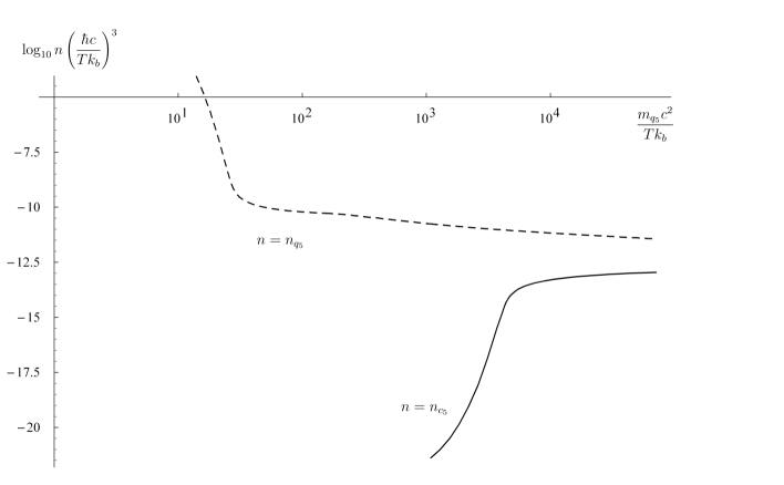
Figure 4: The dependence of the two number densities $n_{q_{5}}$ (of the fifth family quarks) and $n_{c_{5}}$ (of the fifth family clusters) as function of $\frac{m_{q_{5}}\,c^{2}}{k_{b}\,T}$ is presented for the special values $m_{q_{5}}c^{2}=71\,{\rm TeV}$, $\eta_{c_{5}}=\frac{1}{50}$ and $\eta_{(q\bar{q})_{b}}=1$. We take $g^{*}=91.5$. In the treated energy (temperature $k_{b}T$) interval the one gluon exchange gives the main contribution to the scattering cross sections of Eq.(0.14) entering into the Boltzmann equations for $n_{q_{5}}$ and $n_{c_{5}}$. In the figure we make a choice of the parameters within the estimated intervals.

Let us repeat how the $n_{5}$ and $\bar{n}_{5}$ evolve in the evolution of our universe. The quarks and anti-quarks are at high temperature ($\frac{m_{q_{5}}c^{2}}{k_{b}T}<<1$) in thermal equilibrium with the plasma (as are also all the other families and bosons of lower masses). As the temperature of the plasma (due to the expansion of the universe) drops close to the mass of the fifth family quarks, quarks and anti-quarks scatter into all the other (ultra) relativistic fermions and bosons, but can not be created any longer from the plasma (in the average). At the temperature close to the binding energy of the quarks in a cluster, the clusters of the fifth family ($n_{c_{5}},n_{\bar{c}_{5}}$) baryons start to be formed. We evaluated the number density $n_{q_{5}}(T)\,(\frac{\hbar c}{k_{b}T})^{3}=Y_{q_{5}}$ of the fifth family quarks (and anti-quarks) and the number density of the fifth family baryons $n_{c_{5}}(T)\,(\frac{\hbar c}{k_{b}T})^{3}=Y_{c_{5}}$ for several choices of $m_{q_{5}},\eta_{c_{5}}$ and $\eta_{(q\bar{q})_{b}}$ up to $k_{b}T_{lim}=1$ GeV $=\frac{m_{q_{5}}c^{2}}{x_{lim}}$.

From the calculated decoupled number density of baryons and anti-baryons of the fifth family quarks (and anti-quarks) $n_{c_{5}}(T_{1})$ at temperature $k_{b}T_{1}=1$ GeV, where we stopped our calculations as a function of the quark mass and of the two parameters $\eta_{c_{5}}$ and $\eta_{(q\bar{q})_{b}}$, the today’s mass density of the dark matter follows (after taking into account that when once the $n_{5}$ and $\bar{n}_{5}$ decouple, their number stays unchanged but due to the expansion of the universe their density decreases according to $a^{3}_{1}n_{c_{5}}(T_{1})=a^{3}_{2}n_{c_{5}}(T_{2})$, with the today’s $a_{0}=1$ and the temperature $T_{0}=2.725^{0}$ K) leading to gbsnmbdodelson

$$\rho_{dm} = \Omega_{dm}\rho_{cr}=2\,m_{c_{5}}\,n_{c_{5}}(T_{1})\,\left(\frac{T_{0}}{T_{1}}\right)^{3}\frac{g^{*}(T_{1})}{g^{*}(T_{0})},$$ (20)

where we take into account that $g^{*}(T_{1})(a_{1}T_{1})^{3}=g^{*}(T_{0})(a_{0}T_{0})^{3}$, with $T_{0}=2.5\,\cdot 10^{-4}\,\frac{{\rm eV}}{k_{b}}$, $g^{*}(T_{0})=2+\frac{7}{8}\,\cdot 3\,\cdot\,(\frac{4}{11})^{4/3}$, $g^{*}(T_{1})=2+2\,\cdot 8+\frac{7}{8}\,(5\cdot 3\cdot 2\cdot 2+6\cdot 2\cdot 2)$ and $\rho_{cr}\,c^{2}\,\approx\frac{3\,H^{2}_{0}\,c^{2}}{8\pi G}\approx 5.7\,\cdot 10^{3}\frac{{\rm eV}}{{\rm cm}^{3}}$, factor $2$ counts baryons and anti-baryons.

The intervals for the acceptable parameters $\eta_{c_{5}}$ and $\eta_{(q\bar{q})_{b}}$ (determining the inaccuracy, with which the scattering cross sections were evaluated) influence the value of $n_{c_{5}}$ and determine the interval, within which one expects the fifth family mass.

$\frac{m_{q_{5}}c^{2}}{{\rm TeV}}$	$\eta_{(q\bar{q})_{b}}=\frac{1}{10}$	$\eta_{(q\bar{q})_{b}}=\frac{1}{3}$	$\eta_{(q\bar{q})_{b}}=1$	$\eta_{(q\bar{q})_{b}}=3$	$\eta_{(q\bar{q})_{b}}=10$
$\eta_{c_{5}}=\frac{1}{50}$	21	36	71	159	417
$\eta_{c_{5}}=\frac{1}{10}$	12	20	39	84	215
$\eta_{c_{5}}=\frac{1}{3}$	9	14	25	54	134
$\eta_{c_{5}}=1$	8	11	19	37	88
$\eta_{c_{5}}=3$	7	10	15	27	60
$\eta_{c_{5}}=10$	7*	8*	13	22	43

Table 2: The fifth family quark mass is presented (Eq.(20)), calculated for different choices of $\eta_{c_{5}}$ (which takes care of the inaccuracy with which a colourless cluster of three quarks (anti-quarks) cross section was estimated and of $\eta_{(q\bar{q})_{b}}$ (which takes care of the inaccuracy with which the cross section for the annihilation of a bound state of quark—anti-quark was taken into account) from Eqs. (20, 18, 17). * denotes non stable calculations.

We read from Table 2 the mass interval for the fifth family quarks’ mass, which fits Eqs. (20, 18, 17):

$$10\;\;{\rm TeV}<m_{q_{5}}\,c^{2}<{\rm a\,few}\cdot 10^{2}{\rm TeV}.$$ (21)

From this mass interval we estimate from Table 1 the cross section for the fifth family neutrons $\pi(r_{c_{5}})^{2}$:

$$10^{-8}{\rm fm}^{2}\,<\sigma_{c_{5}}<\,10^{-6}{\rm fm}^{2}.$$ (22)

(It is at least $10^{-6}$ smaller than the cross section for the first family neutrons.)

Let us comment on the fifth family quark—anti-quark annihilation at the colour phase transition, which starts at approximately $1$ GeV. When the colour phase transition starts, the quarks start to ”dress” into constituent mass, which brings to them $\approx 300$ MeV/$c^{2}$, since to the force many gluon exchanges start to contribute. The scattering cross sections, which were up to the phase transition dominated by one gluon exchange, rise now to the value of a few ${\rm fm}^{2}$ and more, say $(50{\rm fm})^{2}$. Although the colour phase transition is not yet well understood even for the first family quarks, the evaluation of what happens to the fifth family quarks and anti-quarks and coloured clusters of the fifth family quarks or anti-quarks can still be done as follows. At the interval, when the temperature $k_{b}T$ is considerably above the binding energy of the ”dressed” first family quarks and anti-quarks into mesons or of the binding energy of the three first family quarks or anti-quarks into the first family baryons or anti-baryons, which is $\approx$ a few MeV (one must be more careful with the mesons), the first family quarks and anti-quarks move in the plasma like being free. (Let us remind the reader that the nuclear interaction can be derived as the interaction among the clusters of quarks gbsnmbbmmn .) 25 years ago there were several proposals to treat nuclei as clusters of dressed quarks instead of as clusters of baryons. Although this idea was not very fruitful (since even models with nuclei as bound states of $\alpha$ particles work many a time reasonably) it also was not far from the reality. Accordingly it is meaningful to accept the description of plasma at temperatures above a few $10$ MeV/$k_{b}$ as the plasma of less or more ”dressed” quarks with the very large scattering amplitude (of $\approx(50{\rm fm})^{2}$). The fifth family quarks and anti-quarks, heaving much higher mass (several ten thousands GeV/$c^{2}$ to be compared with $\approx 300$ MeV/$c^{2}$) than the first family quarks and accordingly much higher momentum, ”see” the first family quarks as a ”medium” in which they (the fifth family quarks) scatter among themselves. The fifth family quarks and anti-quarks, having much higher binding energy when forming a meson among themselves than when forming mesons with the first family quarks and anti-quarks (few thousand GeV to be compared with few MeV or few $10$ MeV) and correspondingly very high annihilation probability and also pretty low velocities ($\approx 10^{-3}c$), have during the scattering enough time to annihilate with their anti-particles. The ratio of the scattering time between two coloured quarks (of any kind) and the Hubble time is of the order of $\approx 10^{-18}$ and therefore although the number of the fifth family quarks and anti-quarks is of the order of $10^{-13}$ smaller than the number of the quarks and anti-quarks of the first family (as show the solutions of the Boltzmann equations presented in fig. 4), the fifth family quarks and anti-quarks have in the first period of the colour phase transition (from $\approx$ GeV to $\approx 10$ MeV) enough opportunity to scatter often enough among themselves to deplete (their annihilation time is for several orders of magnitude smaller than the time needed to pass by). More detailed calculations, which are certainly needed, are under considerations. Let us still do rough estimation about the number of the coloured fifth family quarks (and anti-quarks). Using the expression for the thermally averaged cross section for scattering of a quark and an anti-quark and annihilating ($<\sigma v>_{(q\bar{q})_{b}}$ from Eq.(0.14)) and correcting the part which determines the scattering cross section by replacing it with $\eta\,(50{\rm fm})^{2}c\;$ (which takes into account the scattering in the plasma during the colour phase transition in the expanding universe) we obtain the expression $<\sigma v>_{(q\bar{q})_{b}}=\eta_{(q\bar{q})_{b}}\,\eta\,(50{\rm fm})^{2}c\;\sqrt{\frac{E_{c_{5}}}{k_{b}T}}\ln{\frac{E_{c_{5}}}{k_{b}T}}$, which is almost independent of the velocity of the fifth family quarks (which slow down when the temperature lowers). We shall assume that the temperature is lowering as it would be no phase transition and correct this fact with the parameter $\eta$, which could for a few orders of magnitude (say $10^{2}$) enlarge the depleting probability. Using this expression for $<\sigma v>_{(q\bar{q})_{b}}$ in the expression for $\lambda=\frac{<\sigma v>_{(q\bar{q})_{b}}\;m_{q_{5}}c^{2}}{h_{m}(\hbar c)^{3}}$, we obtain for a factor up to $10^{19}$ larger $\lambda$ than it was the one dictating the freeze out procedure of $q_{5}$ and $\bar{q}_{5}$ before the phase transition. Using then the equation $\frac{dY_{q_{5}}}{dx}=\frac{\lambda_{c_{5}}}{x^{2}}\,(-Y^{2}_{q_{5}})$ and integrating it from $Y_{1}$ which is the value from the fig. 4 at $1$ GeV up to the value when $k_{b}T\approx 20$ MeV, when the first family quarks start to bindd into baryons, we obtain in the approximation that $\lambda$ is independent of $x$ (which is not really the case) that $\frac{1}{Y(20{\rm MeV})}=10^{32}\frac{1}{2\cdot 10^{5}}$ or $Y(20{\rm MeV})=10^{-27}$ and correspondingly $n_{q_{5}}(T_{0})=\eta^{-1}10^{-24}cm^{-3}$. Some of these fifth family quarks can form the mesons or baryons and anti-baryons with the first family quarks $q_{1}$ when they start to form baryons and mesons. They would form the anomalous hydrogen in the ratio: $\frac{n_{ah}}{n_{h}}\approx\eta^{-1}\cdot 10^{-12}$, where $n_{ah}$ determines the number of the anomalous (heavy) hydrogen atoms and ${n_{h}}$ the number of the hydrogen atoms, with $\eta$ which might be bellow $10^{2}$. The best measurements in the context of such baryons with the masses of a few hundred TeV/${\rm c}^{2}$ which we were able to find were done $25$ years ago gbsnmbsuperheavy . The authors declare that their measurements manifest that such a ratio should be $\frac{n_{ah}}{n_{h}}<10^{-14}$ for the mass interval between $10$ TeV/$c^{2}$ to $10^{4}$ TeV/$c^{2}$. Our evaluation presented above is very rough and more careful treating the problem might easily lead to lower values than required. On the other side we can not say how trustable is the value for the above ratio for the masses of a few hundreds TeV. Our evaluations are very approximate and if $\eta=10^{2}$ we conclude that the evaluation agrees with measurements.

0.15 Dynamics of a heavy family baryons in our galaxy

There are experiments gbsnmbrita0708 ; gbsnmbcdms which are trying to directly measure the dark matter clusters. Let us make a short introduction into these measurements, treating our fifth family clusters in particular. The density of the dark matter $\rho_{dm}$ in the Milky way can be evaluated from the measured rotation velocity of stars and gas in our galaxy, which appears to be approximately independent of the distance $r$ from the center of our galaxy. For our Sun this velocity is $v_{S}\approx(170-270)$ km/s. $\rho_{dm}$ is approximately spherically symmetric distributed and proportional to $\frac{1}{r^{2}}$. Locally (at the position of our Sun) $\rho_{dm}$ is known within a factor of 10 to be $\rho_{0}\approx 0.3\,{\rm GeV}/(c^{2}\,{\rm cm}^{3})$, we put $\rho_{dm}=\rho_{0}\,\varepsilon_{\rho},$ with $\frac{1}{3}<\varepsilon_{\rho}<3$. The local velocity distribution of the dark matter cluster $\mathchoice{\mbox{\boldmath$\displaystyle v$}}{\mbox{\boldmath$\textstyle v$}}{\mbox{\boldmath$\scriptstyle v$}}{\mbox{\boldmath$\scriptscriptstyle v$}}_{dm\,i}$, in the velocity class $i$ of clusters, can only be estimated, results depend strongly on the model. Let us illustrate this dependence. In a simple model that all the clusters at any radius $r$ from the center of our galaxy travel in all possible circles around the center so that the paths are spherically symmetrically distributed, the velocity of a cluster at the position of the Earth is equal to $v_{S}$, the velocity of our Sun in the absolute value, but has all possible orientations perpendicular to the radius $r$ with equal probability. In the model that the clusters only oscillate through the center of the galaxy, the velocities of the dark matter clusters at the Earth position have values from zero to the escape velocity, each one weighted so that all the contributions give $\rho_{dm}$. Many other possibilities are presented in the references cited in gbsnmbrita0708 .

The velocity of the Earth around the center of the galaxy is equal to: $\mathchoice{\mbox{\boldmath$\displaystyle v$}}{\mbox{\boldmath$\textstyle v$}}{\mbox{\boldmath$\scriptstyle v$}}{\mbox{\boldmath$\scriptscriptstyle v$}}_{E}=\mathchoice{\mbox{\boldmath$\displaystyle v$}}{\mbox{\boldmath$\textstyle v$}}{\mbox{\boldmath$\scriptstyle v$}}{\mbox{\boldmath$\scriptscriptstyle v$}}_{S}+\mathchoice{\mbox{\boldmath$\displaystyle v$}}{\mbox{\boldmath$\textstyle v$}}{\mbox{\boldmath$\scriptstyle v$}}{\mbox{\boldmath$\scriptscriptstyle v$}}_{ES}$, with $v_{ES}=30$ km/s and $\frac{\mathchoice{\mbox{\boldmath$\displaystyle v$}}{\mbox{\boldmath$\textstyle v$}}{\mbox{\boldmath$\scriptstyle v$}}{\mbox{\boldmath$\scriptscriptstyle v$}}_{S}\cdot\mathchoice{\mbox{\boldmath$\displaystyle v$}}{\mbox{\boldmath$\textstyle v$}}{\mbox{\boldmath$\scriptstyle v$}}{\mbox{\boldmath$\scriptscriptstyle v$}}_{ES}}{v_{S}v_{ES}}\approx\cos\theta\,\sin\omega t,\theta=60^{0}$. Then the velocity with which the dark matter cluster of the $i$- th velocity class hits the Earth is equal to: $\mathchoice{\mbox{\boldmath$\displaystyle v$}}{\mbox{\boldmath$\textstyle v$}}{\mbox{\boldmath$\scriptstyle v$}}{\mbox{\boldmath$\scriptscriptstyle v$}}_{dmE\,i}=\mathchoice{\mbox{\boldmath$\displaystyle v$}}{\mbox{\boldmath$\textstyle v$}}{\mbox{\boldmath$\scriptstyle v$}}{\mbox{\boldmath$\scriptscriptstyle v$}}_{dm\,i}-\mathchoice{\mbox{\boldmath$\displaystyle v$}}{\mbox{\boldmath$\textstyle v$}}{\mbox{\boldmath$\scriptstyle v$}}{\mbox{\boldmath$\scriptscriptstyle v$}}_{E}$. $\omega$ determines the rotation of our Earth around the Sun.

One finds for the flux of the dark matter clusters hitting the Earth: $\Phi_{dm}=\sum_{i}\,\frac{\rho_{dm\,i}}{m_{c_{5}}}\,|\mathchoice{\mbox{\boldmath$\displaystyle v$}}{\mbox{\boldmath$\textstyle v$}}{\mbox{\boldmath$\scriptstyle v$}}{\mbox{\boldmath$\scriptscriptstyle v$}}_{dm\,i}-\mathchoice{\mbox{\boldmath$\displaystyle v$}}{\mbox{\boldmath$\textstyle v$}}{\mbox{\boldmath$\scriptstyle v$}}{\mbox{\boldmath$\scriptscriptstyle v$}}_{E}|$ to be approximately (as long as $\frac{v_{ES}}{|\mathchoice{\mbox{\boldmath$\displaystyle v$}}{\mbox{\boldmath$\textstyle v$}}{\mbox{\boldmath$\scriptstyle v$}}{\mbox{\boldmath$\scriptscriptstyle v$}}_{dm\,i}-\mathchoice{\mbox{\boldmath$\displaystyle v$}}{\mbox{\boldmath$\textstyle v$}}{\mbox{\boldmath$\scriptstyle v$}}{\mbox{\boldmath$\scriptscriptstyle v$}}_{S}|}$ is small) equal to

$$\Phi_{dm}\approx\sum_{i}\,\frac{\rho_{dm\,i}}{m_{c_{5}}}\,\{|\mathchoice{\mbox{\boldmath$\displaystyle v$}}{\mbox{\boldmath$\textstyle v$}}{\mbox{\boldmath$\scriptstyle v$}}{\mbox{\boldmath$\scriptscriptstyle v$}}_{dm\,i}-\mathchoice{\mbox{\boldmath$\displaystyle v$}}{\mbox{\boldmath$\textstyle v$}}{\mbox{\boldmath$\scriptstyle v$}}{\mbox{\boldmath$\scriptscriptstyle v$}}_{S}|-\mathchoice{\mbox{\boldmath$\displaystyle v$}}{\mbox{\boldmath$\textstyle v$}}{\mbox{\boldmath$\scriptstyle v$}}{\mbox{\boldmath$\scriptscriptstyle v$}}_{ES}\cdot\frac{\mathchoice{\mbox{\boldmath$\displaystyle v$}}{\mbox{\boldmath$\textstyle v$}}{\mbox{\boldmath$\scriptstyle v$}}{\mbox{\boldmath$\scriptscriptstyle v$}}_{dm\,i}-\mathchoice{\mbox{\boldmath$\displaystyle v$}}{\mbox{\boldmath$\textstyle v$}}{\mbox{\boldmath$\scriptstyle v$}}{\mbox{\boldmath$\scriptscriptstyle v$}}_{S}}{|\mathchoice{\mbox{\boldmath$\displaystyle v$}}{\mbox{\boldmath$\textstyle v$}}{\mbox{\boldmath$\scriptstyle v$}}{\mbox{\boldmath$\scriptscriptstyle v$}}_{dm\,i}-\mathchoice{\mbox{\boldmath$\displaystyle v$}}{\mbox{\boldmath$\textstyle v$}}{\mbox{\boldmath$\scriptstyle v$}}{\mbox{\boldmath$\scriptscriptstyle v$}}_{S}|}\}.$$ (23)

Further terms are neglected. We shall approximately take that

$$\sum_{i}\,|\mathchoice{\mbox{\boldmath$\displaystyle v_{dm\,i}$}}{\mbox{\boldmath$\textstyle v_{dm\,i}$}}{\mbox{\boldmath$\scriptstyle v_{dm\,i}$}}{\mbox{\boldmath$\scriptscriptstyle v_{dm\,i}$}}-\mathchoice{\mbox{\boldmath$\displaystyle v_{S}$}}{\mbox{\boldmath$\textstyle v_{S}$}}{\mbox{\boldmath$\scriptstyle v_{S}$}}{\mbox{\boldmath$\scriptscriptstyle v_{S}$}}|\,\rho_{dm\,i}\approx\varepsilon_{v_{dmS}}\,\varepsilon_{\rho}\,v_{S}\,\rho_{0},$$

and correspondingly $\sum_{i}\,\mathchoice{\mbox{\boldmath$\displaystyle v$}}{\mbox{\boldmath$\textstyle v$}}{\mbox{\boldmath$\scriptstyle v$}}{\mbox{\boldmath$\scriptscriptstyle v$}}_{ES}\cdot\frac{\mathchoice{\mbox{\boldmath$\displaystyle v$}}{\mbox{\boldmath$\textstyle v$}}{\mbox{\boldmath$\scriptstyle v$}}{\mbox{\boldmath$\scriptscriptstyle v$}}_{dm\,i}-\mathchoice{\mbox{\boldmath$\displaystyle v$}}{\mbox{\boldmath$\textstyle v$}}{\mbox{\boldmath$\scriptstyle v$}}{\mbox{\boldmath$\scriptscriptstyle v$}}_{S}}{|\mathchoice{\mbox{\boldmath$\displaystyle v$}}{\mbox{\boldmath$\textstyle v$}}{\mbox{\boldmath$\scriptstyle v$}}{\mbox{\boldmath$\scriptscriptstyle v$}}_{dm\,i}-\mathchoice{\mbox{\boldmath$\displaystyle v$}}{\mbox{\boldmath$\textstyle v$}}{\mbox{\boldmath$\scriptstyle v$}}{\mbox{\boldmath$\scriptscriptstyle v$}}_{S}|}\approx v_{ES}\varepsilon_{v_{dmS}}\cos\theta\,\sin\omega t$, (determining the annual modulations observed by DAMA gbsnmbrita0708 ). Here $\frac{1}{3}<\varepsilon_{v_{dmS}}<3$ and $\frac{1}{3}<\frac{\varepsilon_{v_{dmES}}}{\varepsilon_{v_{dmS}}}<3$ are estimated with respect to experimental and (our) theoretical evaluations.

Let us evaluate the cross section for our heavy dark matter baryon to elastically (the excited states of nuclei, which we shall treat, I and Ge, are at $\approx 50$ keV or higher and are very narrow, while the average recoil energy of Iodine is expected to be $30$ keV) scatter on an ordinary nucleus with $A$ nucleons $\sigma_{A}=\frac{1}{\pi\hbar^{2}}<|M_{c_{5}A}|>^{2}\,m_{A}^{2}$. For our heavy dark matter cluster is $m_{A}$ approximately the mass of the ordinary nucleus . In the case of a coherent scattering (if recognizing that $\lambda=\frac{h}{p_{A}}$ is for a nucleus large enough to make scattering coherent when the mass of the cluster is $1$ TeV or more and its velocity $\approx v_{S}$), the cross section is almost independent of the recoil velocity of the nucleus. For the case that the ”nuclear force” as manifesting in the cross section $\pi\,(r_{c_{5}})^{2}$ in Eq.(15) brings the main contribution  the cross section is proportional to $(3A)^{2}$ (due to the square of the matrix element) times $(A)^{2}$ (due to the mass of the nuclei $m_{A}\approx 3A\,m_{q_{1}}$, with $m_{q_{1}}\,c^{2}\approx\frac{1{\rm GeV}}{3}$). When $m_{q_{5}}$ is heavier than $10^{4}\,{\rm TeV}/c^{2}$ (Table 1), the weak interaction dominates and $\sigma_{A}$ is proportional to $(A-Z)^{2}\,A^{2}$, since to $Z^{0}$ boson exchange only neutron gives an appreciable contribution. Accordingly we have, when the ”nuclear force” dominates, $\sigma_{A}\approx\sigma_{0}\,A^{4}\,\varepsilon_{\sigma}$, with $\sigma_{0}\,\varepsilon_{\sigma}$, which is $\pi r_{c_{5}}^{2}\,\varepsilon_{\sigma_{nucl}}$ and with $\frac{1}{30}<\varepsilon_{\sigma_{nucl}}<30$. $\varepsilon_{\sigma_{nucl}}$ takes into account the roughness with which we treat our heavy baryon’s properties and the scattering procedure. When the weak interaction dominates, $\varepsilon_{\sigma}$ is smaller and we have $\sigma_{0}\,\varepsilon_{\sigma}=(\frac{m_{n_{1}}G_{F}}{\sqrt{2\pi}}\frac{A-Z}{A})^{2}\,\varepsilon_{\sigma_{weak}}$ ($=(10^{-6}\,\frac{A-Z}{A}\,{\rm fm})^{2}\,\varepsilon_{\sigma_{weak}}$), $\frac{1}{10}\,<\,\varepsilon_{\sigma_{weak}}\,<1$. The weak force is pretty accurately evaluated, but the way how we are averaging is not.

0.16 Direct measurements of the fifth family baryons as dark matter constituents

We are making very rough estimations of what the DAMA gbsnmbrita0708 and CDMS gbsnmbcdms experiments are measuring, provided that the dark matter clusters are made out of our (any) heavy family quarks as discussed above. We are looking for limitations these two experiments might put on properties of our heavy family members. We discussed about our estimations and their relations to the measurements with R. Bernabei gbsnmbprivatecommRBJF and J. Filippini gbsnmbprivatecommRBJF . Both pointed out (R.B. in particular) that the two experiments can hardly be compared, and that our very approximate estimations may be right only within the orders of magnitude. We are completely aware of how rough our estimation is, yet we conclude that, since the number of measured events is proportional to $(m_{c_{5}})^{-3}$ for masses $\approx 10^{4}$ TeV or smaller (while for higher masses, when the weak interaction dominates, it is proportional to $(m_{c_{5}})^{-1}$) that even such rough estimations may in the case of our heavy baryons say whether both experiments do at all measure our (any) heavy family clusters, if one experiment clearly sees the dark matter signals and the other does not (yet?) and we accordingly estimate the mass of our cluster.

Let $N_{A}$ be the number of nuclei of a type $A$ in the apparatus (of either DAMA gbsnmbrita0708 , which has $4\cdot 10^{24}$ nuclei per kg of $I$, with $A_{I}=127$, and $Na$, with $A_{Na}=23$ (we shall neglect $Na$), or of CDMS gbsnmbcdms , which has $8.3\cdot 10^{24}$ of $Ge$ nuclei per kg, with $A_{Ge}\approx 73$). At velocities of a dark matter cluster $v_{dmE}$ $\approx$ $200$ km/s are the $3A$ scatterers strongly bound in the nucleus, so that the whole nucleus with $A$ nucleons elastically scatters on a heavy dark matter cluster. Then the number of events per second ($R_{A}$) taking place in $N_{A}$ nuclei is due to the flux $\Phi_{dm}$ and the recognition that the cross section is at these energies almost independent of the velocity equal to

$$R_{A}=\,N_{A}\,\frac{\rho_{0}}{m_{c_{5}}}\;\sigma(A)\,v_{S}\,\varepsilon_{v_{dmS}}\,\varepsilon_{\rho}\,(1+\frac{\varepsilon_{v_{dmES}}}{\varepsilon_{v_{dmS}}}\,\frac{v_{ES}}{v_{S}}\,\cos\theta\,\sin\omega t).$$ (24)

Let $\Delta R_{A}$ mean the amplitude of the annual modulation of $R_{A}$

$$\Delta R_{A} = R_{A}(\omega t=\frac{\pi}{2})-R_{A}(\omega t=0)=N_{A}\,R_{0}\,A^{4}\,\frac{\varepsilon_{v_{dmES}}}{\varepsilon_{v_{dmS}}}\,\frac{v_{ES}}{v_{S}}\,\cos\theta,$$ (25)

where $R_{0}=\sigma_{0}\,\frac{\rho_{0}}{m_{c_{5}}}\,v_{S}\,\varepsilon$, $R_{0}$ is for the case that the ”nuclear force” dominates $R_{0}\approx\pi\,(\frac{3\,\hbar\,c}{\alpha_{c}\,m_{q_{5}}\,c^{2}})^{2}\,\frac{\rho_{0}}{m_{q_{5}}}\,v_{S}\,\varepsilon$, with $\varepsilon=\varepsilon_{\rho}\,\varepsilon_{v_{dmES}}\varepsilon_{\sigma_{nucl}}$. $R_{0}$ is therefore proportional to $m_{q_{5}}^{-3}$. We estimated $10^{-4}<\varepsilon<10$, which demonstrates both, the uncertainties in the knowledge about the dark matter dynamics in our galaxy and our approximate treating of the dark matter properties. (When for $m_{q_{5}}\,c^{2}>10^{4}$ TeV the weak interaction determines the cross section $R_{0}$ is in this case proportional to $m_{q_{5}}^{-1}$.) We estimate that an experiment with $N_{A}$ scatterers should measure the amplitude $R_{A}\varepsilon_{cut\,A}$, with $\varepsilon_{cut\,A}$ determining the efficiency of a particular experiment to detect a dark matter cluster collision. For small enough $\frac{\varepsilon_{v_{dmES}}}{\varepsilon_{v_{dmS}}}\,\frac{v_{ES}}{v_{S}}\,\cos\theta$ we have

$$R_{A}\,\varepsilon_{cut\,A}\approx N_{A}\,R_{0}\,A^{4}\,\varepsilon_{cut\,A}=\Delta R_{A}\varepsilon_{cut\,A}\,\frac{\varepsilon_{v_{dmS}}}{\varepsilon_{v_{dmES}}}\,\frac{v_{S}}{v_{ES}\,\cos\theta}.$$ (26)

If DAMA gbsnmbrita0708 is measuring our heavy family baryons scattering mostly on $I$ (we neglect the same number of $Na$, with $A=23$), then the average $R_{I}$ is

$$R_{I}\varepsilon_{cut\,dama}\approx\Delta R_{dama}\frac{\varepsilon_{v_{dmS}}}{\varepsilon_{v_{dmES}}}\,\frac{v_{S}}{v_{ES}\,\cos 60^{0}},$$ (27)

with $\Delta R_{dama}\approx\Delta R_{I}\,\varepsilon_{cut\,dama}$, this is what we read from their papers gbsnmbrita0708 . In this rough estimation most of unknowns about the dark matter properties, except the local velocity of our Sun, the cut off procedure ($\varepsilon_{cut\,dama}$) and $\frac{\varepsilon_{v_{dmS}}}{\varepsilon_{v_{dmES}}}$, (estimated to be $\frac{1}{3}<\frac{\varepsilon_{v_{dmS}}}{\varepsilon_{v_{dmES}}}<3$), are hidden in $\Delta R_{dama}$. If we assume that the Sun’s velocity is $v_{S}=100,170,220,270$ km/s, we find $\frac{v_{S}}{v_{ES}\cos\theta}=7,10,14,18,$ respectively. (The recoil energy of the nucleus $A=I$ changes correspondingly with the square of $v_{S}$.) DAMA/NaI, DAMA/LIBRA gbsnmbrita0708 publishes $\Delta R_{dama}=0.052$ counts per day and per kg of NaI. Correspondingly is $R_{I}\,\varepsilon_{cut\,dama}=0,052\,\frac{\varepsilon_{v_{dmS}}}{\varepsilon_{v_{dmES}}}\,\frac{v_{S}}{v_{SE}\cos\theta}$ counts per day and per kg. CDMS should then in $121$ days with 1 kg of Ge ($A=73$) detect $R_{Ge}\,\varepsilon_{cut\,cdms}$ $\approx\frac{8.3}{4.0}\,(\frac{73}{127})^{4}\;\frac{\varepsilon_{cut\,cdms}}{\varepsilon_{cut\,dama}}\,\frac{\varepsilon_{v_{dmS}}}{\varepsilon_{v_{dmES}}}\;\frac{v_{S}}{v_{SE}\cos\theta}\;0.052\cdot 121\;$ events, which is for the above measured velocities equal to $(10,16,21,25)\,\frac{\varepsilon_{cut\,cdms}}{\varepsilon_{cut\,dama}}\;\frac{\varepsilon_{v_{dmS}}}{\varepsilon_{v_{dmES}}}$. CDMS gbsnmbcdms has found no event.

The approximations we made might cause that the expected numbers ($10$, $16$, $21$, $25$) multiplied by $\frac{\varepsilon_{cut\,Ge}}{\varepsilon_{cut\,I}}\;\frac{\varepsilon_{v_{dmS}}}{\varepsilon_{v_{dmES}}}$ are too high (or too low!!) for a factor let us say $4$ or $10$. If in the near future CDMS (or some other experiment) will measure the above predicted events, then there might be heavy family clusters which form the dark matter. In this case the DAMA experiment puts the limit on our heavy family masses (Eq.(26)).

Taking into account all the uncertainties mentioned above, with the uncertainty with the ”nuclear force” cross section included (we evaluate these uncertainties to be $10^{-4}<\,\varepsilon^{"}\,<3\cdot 10^{3}$), we can estimate the mass range of the fifth family quarks from the DAMA experiments:

$$(m_{q_{5}}\,c^{2})^{3}=\frac{1}{\Delta R_{dama}}N_{I}\,A^{4}\,\pi\,(\frac{3\,\hbar c}{\alpha_{c}})^{2}\,\rho_{0}\,c^{2}\,v_{ES}\,\cos\theta\,\varepsilon^{"}=(0.3\,\cdot 10^{7})^{3}\,\varepsilon^{"}(\frac{0.1}{\alpha_{c}})^{2}\textrm{GeV}.$$

The lower mass limit, which follows from the DAMA experiment, is accordingly $m_{q_{5}}\,c^{2}>200$ TeV. Observing that for $m_{q_{5}}\,c^{2}>10^{4}$ TeV the weak force starts to dominate, we estimate the upper limit $m_{q_{5}}\,c^{2}<10^{5}$ TeV. Then $200{\rm\;TeV}<m_{q_{5}}\,c^{2}<10^{5}$ TeV.

Let us at the end evaluate the total number of our fifth family neutrons ($n_{5}$) which in $\delta t=121$ days strike $1$ kg of Ge and which CDMS experiment could detect, that is $R_{Ge}\delta t\varepsilon_{cut_{Ge}}=N_{Ge}\sigma_{0}\frac{\rho_{0}}{m_{c_{5}}}\,v_{S}\,A^{4}_{Ge}\,\varepsilon\varepsilon_{cut+{Ge}}$ (Eq. 26), with $N_{Ge}=8.3\cdot 10^{24}$/kg, with the cross section from Table 1, with $A_{Ge}=73$ and $1$ kg of Ge, while $10^{-5}<\varepsilon\varepsilon_{cut_{Ge}}<5\cdot 10$. The coefficient $\varepsilon\varepsilon_{cut_{Ge}}$ determines all the uncertainties: about the scattering amplitudes of the fifth family neutrons on the Ge nuclei (about the scattering amplitude of one $n_{5}$ on the first family quark, about the degree of coherence when scattering on the nuclei, about the local density of the dark matter, about the local velocity of the dark matter and about the efficiency of the experiment). Quite a part of these uncertainties were hidden in the number of events the DAMA/LIBRA experiments measure, when we compare both experiments. If we assume that the fifth family quark mass ($m_{q_{5}}$) is several hundreds TeV, as evaluated (as the upper bound (Eq. 21)) when considering the cosmological history of our fifth family neutrons, we get for the number of events the CDMS experiment should measure: $\varepsilon\varepsilon_{cut_{Ge}}\cdot 10^{4}$. If we take $\varepsilon\varepsilon_{cut_{Ge}}=10^{-5}$, the CDMS experiment should continue to measure 10 times as long as they did.

Let us see how many events CDMS should measure if the dark matter clusters would interact weakly with the Ge nuclei and if the weak interaction would determine also their freezing out procedure, that is if any kind of WIMP would form the dark matter. One easily sees from the Boltzmann equations for the freezing out procedure for $q_{5}$ that since the weak massless boson exchange is approximately hundred times weaker than the one gluon exchange which determines the freeze out procedure of the fifth family quarks, the mass of such an object should be hundred times smaller, which means a few TeV. Taking into account the expression for the weak interaction of such an object with Ge nuclei, which leads to $10^{-2}$ smaller cross section for scattering of one such weakly interacting particle on one proton (see derivations in the previous section), we end up with the number of events which the CDMS experiment should measure: $\varepsilon\varepsilon_{cut_{Ge}}5\cdot 10^{3}$. Since the weak interaction with the matter is much better known that the (”fifth family nuclear force”) interaction of the colourless clusters of $q_{5}$ ($n_{5}$), the $\varepsilon$ is smaller. Let us say $\varepsilon$ is $5\cdot 10^{-4}$. Accordingly, even in the case of weakly interacting dark matter particles the CDMS should continue to measure to see some events.

0.17 Concluding remarks

We estimated in this paper the possibility that a new stable family, predicted by the approach unifying spin and charges gbsnmbpn06 ; gbsnmbn92 ; gbsnmbgmdn07 to have the same charges and the same couplings to the corresponding gauge fields as the known families, forms baryons which are the dark matter constituents. The approach (proposed by S.N.M.B.) is to our knowledge the only proposal in the literature so far which offers the mechanism for generating families, if we do not count those which in one or another way just assume more than three families. Not being able so far to derive from the approach precisely enough the fifth family masses and also not (yet) the baryon asymmetry, we assume that the neutron is the lightest fifth family baryon and that there is no baryon—anti-baryon asymmetry. We comment what changes if the asymmetry exists. We evaluated under these assumptions the properties of the fifth family members in the expanding universe, their clustering into the fifth family neutrons, the scattering of these neutrons on ordinary matter and find the limit on the properties of the stable fifth family quarks due to the cosmological observations and the direct experiments provided that these neutrons constitute the dark matter.

We use the simple hydrogen-like model to evaluate the properties of these heavy baryons and their interaction among themselves and with the ordinary nuclei. We take into account that for masses of the order of $1$ TeV/$c^{2}$ or larger the one gluon exchange determines the force among the constituents of the fifth family baryons. Studying the interaction of these baryons with the ordinary matter we find out that for massive enough fifth family quarks ($m_{q_{5}}>10^{4}$ TeV) the weak interaction starts to dominate over the ”nuclear interaction” which the fifth family neutron manifests. The non relativistic fifth family baryons interact among themselves with the weak force only.

We study the freeze out procedure of the fifth family quarks and anti-quarks and the formation of baryons and anti-baryons up to the temperature $k_{b}T=1$ GeV, when the colour phase transition starts which to our estimations depletes almost all the fifth family quarks and anti-quarks while the colourless fifth family neutrons with very small scattering cross section decouples long before (at $k_{b}T=100$ GeV).

The cosmological evolution suggests for the mass limits the range $10$ TeV $<m_{q_{5}}\,c^{2}<{\rm a\,few}\cdot 10^{2}$ TeV and for the scattering cross sections $10^{-8}\,{\rm fm}^{2}\,<\sigma_{c_{5}}\,<10^{-6}\,{\rm fm}^{2}$. The measured density of the dark matter does not put much limitation on the properties of heavy enough clusters.

The DAMA experiments gbsnmbrita0708 limit (provided that they measure our heavy fifth family clusters) the quark mass to: $200\,{\rm TeV}<m_{q_{5}}c^{2}<10^{5}\,{\rm TeV}$. The estimated cross section for the dark matter cluster to (elastically, coherently and nonrelativisically) scatter on the (first family) nucleus is in this case determined on the lower mass limit by the ”fifth family nuclear force” of the fifth family clusters ($(3\cdot 10^{-5}\,A^{2}\,{\rm fm})^{2}$) and on the higher mass limit by the weak force ($(A(A-Z)\,10^{-6}\,{\rm fm})^{2}$). Accordingly we conclude that if the DAMA experiments are measuring our fifth family neutrons, the mass of the fifth family quarks is a few hundred TeV $/c^{2}$.

Taking into account all the uncertainties in connection with the dark matter clusters (the local density of the dark matter and its local velocity) including the scattering cross sections of our fifth family neutrons on the ordinary nuclei as well as the experimental errors, we do expect that CDMS will in a few years measure our fifth family baryons.

Let us point out that the stable fifth family neutrons are not the WIMPS, which would interact with the weak force only: the cosmological behaviour (the freezing out procedure) of these clusters are dictated by the colour force, while their interaction with the ordinary matter is determined by the ”fifth family nuclear force” if they have masses smaller than $10^{4}$ TeV/$c^{2}$.

In the ref. gbsnmbmbb   the authors study the limits on a scattering cross section of a heavy dark matter cluster of particles and anti-particles (both of approximately the same amount) with the ordinary matter, estimating the energy flux produced by the annihilation of such pairs of clusters. They treat the conditions under which would the heat flow following from the annihilation of dark matter particles and anti-particles in the Earth core start to be noticeable. Using their limits we conclude that our fifth family baryons of the mass of a few hundreds TeV/${c^{2}}$ have for a factor more than $100$ too small scattering amplitude with the ordinary matter to cause a measurable heat flux on the Earth’s surface. On the other hand could the measurements gbsnmbsuperheavy tell whether the fifth family members do deplete at the colour phase transition of our universe enough to be in agreement with them. Our very rough estimation show that the fifth family members are on the allowed limit, but they are too rough to be taken as a real limit.

Our estimations predict that, if the DAMA experiments observe the events due to our (any) heavy family members, (or any heavy enough family clusters with small enough cross section), the CDMS experiments gbsnmbcdms will in the near future observe a few events as well. If CDMS will not confirm the heavy family events, then we must conclude, trusting the DAMA experiments, that either our fifth family clusters have much higher cross section due to the possibility that $u_{5}$ is lighter than $d_{5}$ so that their velocity slows down when scattering on nuclei of the earth above the measuring apparatus bellow the threshold of the CDMS experiment (and that there must be in this case the fifth family quarks—anti-quarks asymmetry) gbsnmbmaxim ) while the DAMA experiment still observes them, or the fifth family clusters (any heavy stable family clusters) are not what forms the dark matter.

Let us comment again the question whether it is at all possible (due to electroweak experimental data) that there exist more than three up to now observed families, that is, whether the approach unifying spin and charges by predicting the fourth and the stable fifth family (with neutrinos included) contradict the observations. In the ref. gbsnmbmdnbled06 the properties of all the members of the fourth family were studied (for one particular choice of breaking the starting symmetry). The predicted fourth family neutrino mass is at around $100$ GeV/$c^{2}$ or higher, therefore it does not due to the detailed analyses of the electroweak data done by the Russian group gbsnmbokun contradict any experimental data. The stable fifth family neutrino has due to our calculations considerably higher mass. Accordingly none of these two neutrinos contradict the electroweak data. They also do not contradict the nucleosynthesis, since to the nucleosynthesis only the neutrinos with masses bellow the electron mass contribute. The fact that the fifth family baryons might form the dark matter does not contradict the measured (first family) baryon number and its ratio to the photon energy density as well, as long as the fifth family quarks are heavy enough ($>$1 TeV). All the measurements, which connect the baryon and the photon energy density, relate to the moment(s) in the history of the universe, when the baryons (of the first family) where formed ($m_{1}c^{2}\approx k_{b}T=1$ GeV and lower) and the electrons and nuclei were forming atoms ($k_{b}\,T\approx 1$ eV). The chargeless (with respect to the colour and electromagnetic charges, not with respect to the weak charge) clusters of the fifth family were formed long before (at $k_{b}T\approx E_{c_{5}}$ (Table 1)). They manifest after decoupling from the plasma (with their small number density and small cross section) (almost) only their gravitational interaction.

Let the reader recognize that the fifth family baryons are not the objects—WIMPS—which would interact with only the weak interaction, since their decoupling from the rest of the plasma in the expanding universe is determined by the colour force and their interaction with the ordinary matter is determined with the fifth family ”nuclear force” (the force among the fifth family nucleons, manifesting much smaller cross section than does the ordinary ”nuclear force”) as long as their mass is not higher than $10^{4}$ TeV, when the weak interaction starts to dominate as commented in section 0.15.

Let us conclude this paper with the recognition: If the approach unifying spin and charges is the right way beyond the standard model of the electroweak and colour interaction, then more than three families of quarks and leptons do exist, and the stable (with respect to the age of the universe) fifth family of quarks and leptons is the candidate to form the dark matter. The assumptions we made (i. The fifth family neutron is the lightest fifth family baryon, ii. There is no fifth family baryon asymmetry), could be derived from the approach unifying spins and charges and we are working on these problems. The fifth family baryon anti-baryon asymmetry does not very much change the conclusions of this paper as long as the fifth family quarks’s mass is a few hundreds TeV or higher.

0.18 Appendix: Three fifth family quarks’ bound states

We look for the ground state solution of the Hamilton equation $H\,|\psi\rangle=E_{c_{5}}\,|\psi\rangle$ for a cluster of three heavy quarks with

$$H=\sum_{i=1}^{3}\,\frac{p_{i}^{2}}{2\,m_{q_{5}}}-\frac{2}{3}\,\,\sum_{i<j=1}^{3}\frac{\hbar c\;\alpha_{c}}{|\mathchoice{\mbox{\boldmath$\displaystyle x$}}{\mbox{\boldmath$\textstyle x$}}{\mbox{\boldmath$\scriptstyle x$}}{\mbox{\boldmath$\scriptscriptstyle x$}}_{i}-\mathchoice{\mbox{\boldmath$\displaystyle x$}}{\mbox{\boldmath$\textstyle x$}}{\mbox{\boldmath$\scriptstyle x$}}{\mbox{\boldmath$\scriptscriptstyle x$}}_{j}|},$$ (28)

in the center of mass motion

$$\mathchoice{\mbox{\boldmath$\displaystyle x$}}{\mbox{\boldmath$\textstyle x$}}{\mbox{\boldmath$\scriptstyle x$}}{\mbox{\boldmath$\scriptscriptstyle x$}}=\mathchoice{\mbox{\boldmath$\displaystyle x$}}{\mbox{\boldmath$\textstyle x$}}{\mbox{\boldmath$\scriptstyle x$}}{\mbox{\boldmath$\scriptscriptstyle x$}}_{2}-\mathchoice{\mbox{\boldmath$\displaystyle x$}}{\mbox{\boldmath$\textstyle x$}}{\mbox{\boldmath$\scriptstyle x$}}{\mbox{\boldmath$\scriptscriptstyle x$}}_{1},\quad\mathchoice{\mbox{\boldmath$\displaystyle y$}}{\mbox{\boldmath$\textstyle y$}}{\mbox{\boldmath$\scriptstyle y$}}{\mbox{\boldmath$\scriptscriptstyle y$}}=\mathchoice{\mbox{\boldmath$\displaystyle x$}}{\mbox{\boldmath$\textstyle x$}}{\mbox{\boldmath$\scriptstyle x$}}{\mbox{\boldmath$\scriptscriptstyle x$}}_{3}-\frac{\mathchoice{\mbox{\boldmath$\displaystyle x$}}{\mbox{\boldmath$\textstyle x$}}{\mbox{\boldmath$\scriptstyle x$}}{\mbox{\boldmath$\scriptscriptstyle x$}}_{1}+\mathchoice{\mbox{\boldmath$\displaystyle x$}}{\mbox{\boldmath$\textstyle x$}}{\mbox{\boldmath$\scriptstyle x$}}{\mbox{\boldmath$\scriptscriptstyle x$}}_{2}}{2},\quad\mathchoice{\mbox{\boldmath$\displaystyle R$}}{\mbox{\boldmath$\textstyle R$}}{\mbox{\boldmath$\scriptstyle R$}}{\mbox{\boldmath$\scriptscriptstyle R$}}=\frac{\mathchoice{\mbox{\boldmath$\displaystyle x$}}{\mbox{\boldmath$\textstyle x$}}{\mbox{\boldmath$\scriptstyle x$}}{\mbox{\boldmath$\scriptscriptstyle x$}}_{1}+\mathchoice{\mbox{\boldmath$\displaystyle x$}}{\mbox{\boldmath$\textstyle x$}}{\mbox{\boldmath$\scriptstyle x$}}{\mbox{\boldmath$\scriptscriptstyle x$}}_{2}+\mathchoice{\mbox{\boldmath$\displaystyle x$}}{\mbox{\boldmath$\textstyle x$}}{\mbox{\boldmath$\scriptstyle x$}}{\mbox{\boldmath$\scriptscriptstyle x$}}_{3}}{3},$$ (29)

assuming the anti-symmetric colour part ($|\psi\rangle_{c,\,\cal{A}}$), symmetric spin and weak charge part ($|\psi\rangle_{w\,{\rm spin},\,\cal{S}}$) and symmetric space part ($|\psi\rangle_{{\rm space},\,\cal{S}}$). For the space part we take the hydrogen-like wave functions $\psi_{a}(\mathchoice{\mbox{\boldmath$\displaystyle x$}}{\mbox{\boldmath$\textstyle x$}}{\mbox{\boldmath$\scriptstyle x$}}{\mbox{\boldmath$\scriptscriptstyle x$}})=$$\frac{1}{\sqrt{\pi a^{3}}}\;e^{-|\mathchoice{\mbox{\boldmath$\displaystyle x$}}{\mbox{\boldmath$\textstyle x$}}{\mbox{\boldmath$\scriptstyle x$}}{\mbox{\boldmath$\scriptscriptstyle x$}}|/a}$ and $\psi_{b}(\mathchoice{\mbox{\boldmath$\displaystyle y$}}{\mbox{\boldmath$\textstyle y$}}{\mbox{\boldmath$\scriptstyle y$}}{\mbox{\boldmath$\scriptscriptstyle y$}})=$$\frac{1}{\sqrt{\pi b^{3}}}\;e^{-|\mathchoice{\mbox{\boldmath$\displaystyle y$}}{\mbox{\boldmath$\textstyle y$}}{\mbox{\boldmath$\scriptstyle y$}}{\mbox{\boldmath$\scriptscriptstyle y$}}|/b}$, allowing $a$ and $b$ to adapt variationally. Accordingly

$$\langle\,\mathchoice{\mbox{\boldmath$\displaystyle x$}}{\mbox{\boldmath$\textstyle x$}}{\mbox{\boldmath$\scriptstyle x$}}{\mbox{\boldmath$\scriptscriptstyle x$}}_{1},\mathchoice{\mbox{\boldmath$\displaystyle x$}}{\mbox{\boldmath$\textstyle x$}}{\mbox{\boldmath$\scriptstyle x$}}{\mbox{\boldmath$\scriptscriptstyle x$}}_{2},\mathchoice{\mbox{\boldmath$\displaystyle x$}}{\mbox{\boldmath$\textstyle x$}}{\mbox{\boldmath$\scriptstyle x$}}{\mbox{\boldmath$\scriptscriptstyle x$}}_{3}|\psi\rangle_{{\rm space}\,\cal{S}}=\mathcal{N}\left(\psi_{a}(\mathchoice{\mbox{\boldmath$\displaystyle x$}}{\mbox{\boldmath$\textstyle x$}}{\mbox{\boldmath$\scriptstyle x$}}{\mbox{\boldmath$\scriptscriptstyle x$}})\psi_{b}(\mathchoice{\mbox{\boldmath$\displaystyle y$}}{\mbox{\boldmath$\textstyle y$}}{\mbox{\boldmath$\scriptstyle y$}}{\mbox{\boldmath$\scriptscriptstyle y$}})+\textrm{symmetric permutations}\right).$$

It follows

$$\langle\,\mathchoice{\mbox{\boldmath$\displaystyle x$}}{\mbox{\boldmath$\textstyle x$}}{\mbox{\boldmath$\scriptstyle x$}}{\mbox{\boldmath$\scriptscriptstyle x$}}_{1},\mathchoice{\mbox{\boldmath$\displaystyle x$}}{\mbox{\boldmath$\textstyle x$}}{\mbox{\boldmath$\scriptstyle x$}}{\mbox{\boldmath$\scriptscriptstyle x$}}_{2},\mathchoice{\mbox{\boldmath$\displaystyle x$}}{\mbox{\boldmath$\textstyle x$}}{\mbox{\boldmath$\scriptstyle x$}}{\mbox{\boldmath$\scriptscriptstyle x$}}_{3}|\psi\rangle_{{\rm space}\,\cal{S}}=\\ \mathcal{N}\,\bigl{(}2\psi_{a}(\mathchoice{\mbox{\boldmath$\displaystyle x$}}{\mbox{\boldmath$\textstyle x$}}{\mbox{\boldmath$\scriptstyle x$}}{\mbox{\boldmath$\scriptscriptstyle x$}})\psi_{b}(\mathchoice{\mbox{\boldmath$\displaystyle y$}}{\mbox{\boldmath$\textstyle y$}}{\mbox{\boldmath$\scriptstyle y$}}{\mbox{\boldmath$\scriptscriptstyle y$}})+2\psi_{a}(\mathchoice{\mbox{\boldmath$\displaystyle y$}}{\mbox{\boldmath$\textstyle y$}}{\mbox{\boldmath$\scriptstyle y$}}{\mbox{\boldmath$\scriptscriptstyle y$}}-\frac{\mathchoice{\mbox{\boldmath$\displaystyle x$}}{\mbox{\boldmath$\textstyle x$}}{\mbox{\boldmath$\scriptstyle x$}}{\mbox{\boldmath$\scriptscriptstyle x$}}}{2})\psi_{b}(\frac{\mathchoice{\mbox{\boldmath$\displaystyle y$}}{\mbox{\boldmath$\textstyle y$}}{\mbox{\boldmath$\scriptstyle y$}}{\mbox{\boldmath$\scriptscriptstyle y$}}}{2}+\frac{3\mathchoice{\mbox{\boldmath$\displaystyle x$}}{\mbox{\boldmath$\textstyle x$}}{\mbox{\boldmath$\scriptstyle x$}}{\mbox{\boldmath$\scriptscriptstyle x$}}}{4}))+2\psi_{a}(\mathchoice{\mbox{\boldmath$\displaystyle y$}}{\mbox{\boldmath$\textstyle y$}}{\mbox{\boldmath$\scriptstyle y$}}{\mbox{\boldmath$\scriptscriptstyle y$}}+\frac{\mathchoice{\mbox{\boldmath$\displaystyle x$}}{\mbox{\boldmath$\textstyle x$}}{\mbox{\boldmath$\scriptstyle x$}}{\mbox{\boldmath$\scriptscriptstyle x$}}}{2})\psi_{b}(\frac{\mathchoice{\mbox{\boldmath$\displaystyle y$}}{\mbox{\boldmath$\textstyle y$}}{\mbox{\boldmath$\scriptstyle y$}}{\mbox{\boldmath$\scriptscriptstyle y$}}}{2}-\frac{3\mathchoice{\mbox{\boldmath$\displaystyle x$}}{\mbox{\boldmath$\textstyle x$}}{\mbox{\boldmath$\scriptstyle x$}}{\mbox{\boldmath$\scriptscriptstyle x$}}}{4})\bigr{)}.$$ (30)

The Hamiltonian in the center of mass motion reads $H=\frac{p_{x}^{2}}{2(\frac{m_{q_{5}}}{2})}+\frac{p_{y}^{2}}{2(\frac{2m_{q_{5}}}{3})}+\frac{p_{R}^{2}}{2\cdot 3m_{q_{5}}}-\frac{2}{3}\hbar c\;\alpha_{c}\left(\frac{1}{x}+\frac{1}{|\mathchoice{\mbox{\boldmath$\displaystyle y$}}{\mbox{\boldmath$\textstyle y$}}{\mbox{\boldmath$\scriptstyle y$}}{\mbox{\boldmath$\scriptscriptstyle y$}}+\frac{\mathchoice{\mbox{\boldmath$\displaystyle x$}}{\mbox{\boldmath$\textstyle x$}}{\mbox{\boldmath$\scriptstyle x$}}{\mbox{\boldmath$\scriptscriptstyle x$}}}{2}|}+\frac{1}{|\mathchoice{\mbox{\boldmath$\displaystyle y$}}{\mbox{\boldmath$\textstyle y$}}{\mbox{\boldmath$\scriptstyle y$}}{\mbox{\boldmath$\scriptscriptstyle y$}}-\frac{\mathchoice{\mbox{\boldmath$\displaystyle x$}}{\mbox{\boldmath$\textstyle x$}}{\mbox{\boldmath$\scriptstyle x$}}{\mbox{\boldmath$\scriptscriptstyle x$}}}{2}|}\right).$ Varying the expectation value of the Hamiltonian with respect to $a$ and $b$ it follows: $\frac{a}{b}=1.03,\,\frac{a\,\alpha_{c}\,m_{q_{5}}\,c^{2}}{\hbar c}=1.6$.

Accordingly we get for the binding energy $E_{c_{5}}=0.66\;m_{q_{5}}\,c^{2}\alpha_{c}^{2}$ and for the size of the cluster $\sqrt{\langle|\mathchoice{\mbox{\boldmath$\displaystyle x$}}{\mbox{\boldmath$\textstyle x$}}{\mbox{\boldmath$\scriptstyle x$}}{\mbox{\boldmath$\scriptscriptstyle x$}}_{2}-\mathchoice{\mbox{\boldmath$\displaystyle x$}}{\mbox{\boldmath$\textstyle x$}}{\mbox{\boldmath$\scriptstyle x$}}{\mbox{\boldmath$\scriptscriptstyle x$}}_{1}|^{2}\rangle}=2.5\,\frac{\hbar c}{\alpha_{c}m_{q_{5}\,c^{2}}}$.

To estimate the mass difference between $u_{5}$ and $d_{5}$ for which $u_{5}d_{5}d_{5}$ is stable we treat the electromagnetic ($\alpha_{elm}$) and weak ($\alpha_{w}$) interaction as a small correction to the above calculated binding energy: $H^{\prime}=\alpha_{elm\,w}\;\hbar c\,\left(\frac{1}{x}+\frac{1}{|\mathchoice{\mbox{\boldmath$\displaystyle y$}}{\mbox{\boldmath$\textstyle y$}}{\mbox{\boldmath$\scriptstyle y$}}{\mbox{\boldmath$\scriptscriptstyle y$}}+\frac{\mathchoice{\mbox{\boldmath$\displaystyle x$}}{\mbox{\boldmath$\textstyle x$}}{\mbox{\boldmath$\scriptstyle x$}}{\mbox{\boldmath$\scriptscriptstyle x$}}}{2}|}+\frac{1}{|\mathchoice{\mbox{\boldmath$\displaystyle y$}}{\mbox{\boldmath$\textstyle y$}}{\mbox{\boldmath$\scriptstyle y$}}{\mbox{\boldmath$\scriptscriptstyle y$}}-\frac{\mathchoice{\mbox{\boldmath$\displaystyle x$}}{\mbox{\boldmath$\textstyle x$}}{\mbox{\boldmath$\scriptstyle x$}}{\mbox{\boldmath$\scriptscriptstyle x$}}}{2}|}\right)$. $\alpha_{elm\,w}$ stays for electromagnetic and weak coupling constants. For $m_{q_{5}}=200$ TeV we take $\alpha_{elm\,w}=\frac{1}{100}$, then $|m_{u_{5}}-m_{d_{5}}|<\frac{1}{3}\,E_{c_{5}}\frac{(\frac{3}{2}\alpha_{elm\,w})^{2}}{\alpha_{c}^{2}}=0.5\,\cdot 10^{-4}\;m_{q_{5}}\,c^{2}$.

V.V. Dvoeglazov P, C and T for Truly Neutral ParticlesPresented at the QTRF-5, Växjö. Sweden, June 14-18, 2009 and at the ICSSUR09, Olomouc, Czech Republic, June 22-26, 2009. The extended version is contributed to the 12th International Workshop ’What Comes Beyond the Standard Models’, 14. - 24. July 2009, Bled.

During the 20th century various authors introduced self/anti-self charge-conjugate 4-spinors (including in the momentum representation), see vd1Majorana ; vd1Bilenky ; vd1Ziino ; vd1Ahluwalia . Later, Lounesto, Dvoeglazov, Kirchbach etc studied these spinors, they found dynamical equations, gauge transformations and other specific features of them. Recently, in vd1Kirchbach it was claimed that “for imaginary $C$ parities, the neutrino mass can drop out from the single $\beta$ decay trace and reappear in $0\nu\beta\beta$,… in principle experimentally testable signature for a non-trivial impact of Majorana framework in experiments with polarized sources” (see also Summary of the cited paper). Thus, phase factors can have physical significance in quantum mechanics. So, the aim of my talk is to remind what several researchers presented in the 90s concerning with the neutrino description.

The definitions are:

$$C=e^{i\theta_{c}}\begin{pmatrix}0&0&0&-i\\ 0&0&i&0\\ 0&i&0&0\\ -i&0&0&0\end{pmatrix}{\cal K}=-e^{i\theta_{c}}\gamma^{2}{\cal K}$$ (31)

is the anti-linear operator of charge conjugation. We define the self/anti-self charge-conjugate 4-spinors in the momentum space

$$C\lambda^{S,A}(p^{\mu}) = \pm\lambda^{S,A}(p^{\mu})\,,$$ (32)

$$C\rho^{S,A}(p^{\mu}) = \pm\rho^{S,A}(p^{\mu})\,,$$ (33)

where

$$\lambda^{S,A}(p^{\mu})=\begin{pmatrix}\pm i\Theta\phi^{\ast}_{L}(p^{\mu})\\ \phi_{L}(p^{\mu})\end{pmatrix}$$ (34)

and

$$\rho^{S,A}(p^{\mu})=\begin{pmatrix}\phi_{R}(p^{\mu})\\ \mp i\Theta\phi^{\ast}_{R}(p^{\mu})\end{pmatrix}\,.$$ (35)

The Wigner matrix is

$$\Theta_{[1/2]}=-i\sigma_{2}=\begin{pmatrix}0&-1\\ 1&0\end{pmatrix}\,,$$ (36)

and $\phi_{L}$, $\phi_{R}$ are the Ryder (Weyl) left- and right-handed 2-spinors

$$\phi_{R}(p^{\mu}) = \Lambda_{R}({\bf p}\leftarrow{\bf 0})\phi_{R}({\bf 0})=\exp(+{\mathbf{\sigma}}\cdot{\mathbf{\varphi}}/2)\phi_{R}({\bf 0})\,,$$ (37)

$$\phi_{L}(p^{\mu}) = \Lambda_{L}{\bf p}\leftarrow{\bf 0})\phi_{L}({\bf 0})=\exp(-{\mathbf{\sigma}}\cdot{\mathbf{\varphi}}/2)\phi_{L}({\bf 0})\,,$$ (38)

with ${\mathbf{\varphi}}={\bf n}\varphi$ being the boost parameters:

$$cosh\varphi=\gamma=\frac{1}{\sqrt{1-v^{2}/c^{2}}}\,,\,sinh\varphi=\beta\gamma=\frac{v/c}{\sqrt{1-v^{2}/c^{2}}}\,,\,tanh\varphi=v/c\,.$$ (39)

As we have shown the 4-spinors $\lambda$ and $\rho$ are NOT the eigenspinors of helicity. Moreover, $\lambda$ and $\rho$ are NOT the eigenspinors of the parity $P=\begin{pmatrix}0&1\\ 1&0\end{pmatrix}R$, as opposed to the Dirac case.

Such definitions of 4-spinors differ, of course, from the original Majorana definition in x-representation:

$$\nu(x)=\frac{1}{\sqrt{2}}(\Psi_{D}(x)+\Psi_{D}^{c}(x))\,,$$ (40)

$$\nu(x)=\int\frac{d^{3}{\bf p}}{(2\pi)^{3}2E_{p}}\sum_{\sigma}[u_{\sigma}({\bf p})a_{\sigma}({\bf p})e^{-ip\cdot x}+v_{\sigma}({\bf p})[\lambda a_{\sigma}^{\dagger}({\bf p})]e^{+ip\cdot x}]\,,$$ (41)

$$a_{\sigma}({\bf p})=\frac{1}{\sqrt{2}}(b_{\sigma}({\bf p})+d_{\sigma}^{\dagger}({\bf p}))\,,$$ (42)

$C\nu(x)=\nu(x)$ that represents the positive real $C-$ parity field operator. However, the momentum-space Majorana-like spinors open various possibilities for description of neutral particles (with experimental consequences, see vd1Kirchbach ).

The 4-spinors of the second kind $\lambda^{S,A}_{\uparrow\downarrow}(p^{\mu})$ and $\rho^{S,A}_{\uparrow\downarrow}(p^{\mu})$ are vd1Dvoeglazov2 :

$$\lambda^{S}_{\uparrow}(p^{\mu})=\frac{1}{2\sqrt{E+m}}\begin{pmatrix}ip_{l}\\ i(p^{-}+m)\\ p^{-}+m\\ -p_{r}\end{pmatrix},\lambda^{S}_{\downarrow}(p^{\mu})=\frac{1}{2\sqrt{E+m}}\begin{pmatrix}-i(p^{+}+m)\\ -ip_{r}\\ -p_{l}\\ (p^{+}+m)\end{pmatrix},$$ (43)

$$\lambda^{A}_{\uparrow}(p^{\mu})=\frac{1}{2\sqrt{E+m}}\begin{pmatrix}-ip_{l}\\ -i(p^{-}+m)\\ (p^{-}+m)\\ -p_{r}\end{pmatrix},\lambda^{A}_{\downarrow}(p^{\mu})=\frac{1}{2\sqrt{E+m}}\begin{pmatrix}i(p^{+}+m)\\ ip_{r}\\ -p_{l}\\ (p^{+}+m)\end{pmatrix},$$ (44)

$$\rho^{S}_{\uparrow}(p^{\mu})=\frac{1}{2\sqrt{E+m}}\begin{pmatrix}p^{+}+m\\ p_{r}\\ ip_{l}\\ -i(p^{+}+m)\end{pmatrix},\rho^{S}_{\downarrow}(p^{\mu})=\frac{1}{2\sqrt{E+m}}\begin{pmatrix}p_{l}\\ (p^{-}+m)\\ i(p^{-}+m)\\ -ip_{r}\end{pmatrix},$$ (45)

$$\rho^{A}_{\uparrow}(p^{\mu})=\frac{1}{2\sqrt{E+m}}\begin{pmatrix}p^{+}+m\\ p_{r}\\ -ip_{l}\\ i(p^{+}+m)\end{pmatrix},\rho^{A}_{\downarrow}(p^{\mu})=\frac{1}{2\sqrt{E+m}}\begin{pmatrix}p_{l}\\ (p^{-}+m)\\ -i(p^{-}+m)\\ ip_{r}\end{pmatrix}$$ (46)

with $p_{r}=p_{x}+ip_{y}$, $p_{l}=p_{x}-ip_{y}$, $p^{\pm}=p_{0}\pm p_{z}$. The indices $\uparrow\downarrow$ should be referred to either the chiral helicity quantum number introduced in the 60s, $\eta=-\gamma^{5}h$ or to the $\hat{S}_{3}$ operator quantum numbers. While

$$Pu_{\sigma}({\bf p})=+u_{\sigma}({\bf p})\,,Pv_{\sigma}({\bf p})=-v_{\sigma}({\bf p})\,,$$ (47)

we have

$$P\lambda^{S,A}({\bf p})=\rho^{A,S}({\bf p})\,,P\rho^{S,A}({\bf p})=\lambda^{A,S}({\bf p})\,,$$ (48)

for the Majorana-like momentum-space 4-spinors on the first quantization level. In this basis one has

$$\rho^{S}_{\uparrow}(p^{\mu})\, = \,-i\lambda^{A}_{\downarrow}(p^{\mu})\,,\,\rho^{S}_{\downarrow}(p^{\mu})\,=\,+i\lambda^{A}_{\uparrow}(p^{\mu})\,,$$ (49)

$$\rho^{A}_{\uparrow}(p^{\mu})\, = \,+i\lambda^{S}_{\downarrow}(p^{\mu})\,,\,\rho^{A}_{\downarrow}(p^{\mu})\,=\,-i\lambda^{S}_{\uparrow}(p^{\mu})\,.$$ (50)

The normalization of the spinors $\lambda^{S,A}_{\uparrow\downarrow}(p^{\mu})$ and $\rho^{S,A}_{\uparrow\downarrow}(p^{\mu})$ are the following ones:

$$\overline{\lambda}^{S}_{\uparrow}(p^{\mu})\lambda^{S}_{\downarrow}(p^{\mu})\, = \,-im\,,\,\overline{\lambda}^{S}_{\downarrow}(p^{\mu})\lambda^{S}_{\uparrow}(p^{\mu})\,=\,+im\,,$$ (51)

$$\overline{\lambda}^{A}_{\uparrow}(p^{\mu})\lambda^{A}_{\downarrow}(p^{\mu})\, = \,+im\,,\,\overline{\lambda}^{A}_{\downarrow}(p^{\mu})\lambda^{A}_{\uparrow}(p^{\mu})\,=\,-im\,,$$ (52)

$$\overline{\rho}^{S}_{\uparrow}(p^{\mu})\rho^{S}_{\downarrow}(p^{\mu})\, = \,+im\,,\,\overline{\rho}^{S}_{\downarrow}(p^{\mu})\rho^{S}_{\uparrow}(p^{\mu})\,=\,-im\,,$$ (53)

$$\overline{\rho}^{A}_{\uparrow}(p^{\mu})\rho^{A}_{\downarrow}(p^{\mu})\, = \,-im\,,\,\overline{\rho}^{A}_{\downarrow}(p^{\mu})\rho^{A}_{\uparrow}(p^{\mu})\,=\,+im\,.$$ (54)

All other conditions are equal to zero.

First of all, one must derive dynamical equations for the Majorana-like spinors in order to see what dynamics do the neutral particles have. One can use the generalized form of the Ryder relation for zero-momentum spinors:

$$\left[\phi_{{}_{L}}^{h}({\bf 0})\right]^{*}=(-1)^{1/2-h}\,e^{-i(\vartheta_{1}^{L}+\vartheta_{2}^{L})}\,\Theta_{[1/2]}\,\phi_{{}_{L}}^{-h}({\bf 0})\,,$$ (55)

Relations for zero-momentum right spinors are obtained with the substitution $L\leftrightarrow R$. $h$ is the helicity quantum number for the left- and right 2-spinors. Hence, implying that $\lambda^{S}(p^{\mu})$ (and $\rho^{A}(p^{\mu})$) answer for positive-frequency solutions; $\lambda^{A}(p^{\mu})$ (and $\rho^{S}(p^{\mu})$), for negative-frequency solutions, one can obtain the dynamical coordinate-space equations vd1Dvoeglazov1

$$i\gamma^{\mu}\partial_{\mu}\lambda^{S}(x)-m\rho^{A}(x) = 0\,,$$ (56)

$$i\gamma^{\mu}\partial_{\mu}\rho^{A}(x)-m\lambda^{S}(x) = 0\,,$$ (57)

$$i\gamma^{\mu}\partial_{\mu}\lambda^{A}(x)+m\rho^{S}(x) = 0\,,$$ (58)

$$i\gamma^{\mu}\partial_{\mu}\rho^{S}(x)+m\lambda^{A}(x) = 0\,.$$ (59)

These are NOT the Dirac equations.

They can be written in the 8-component form as follows:

$$\left[i\Gamma^{\mu}\partial_{\mu}-m\right]\Psi_{{}_{(+)}}(x) = 0\,,$$ (60)

$$\left[i\Gamma^{\mu}\partial_{\mu}+m\right]\Psi_{{}_{(-)}}(x) = 0\,,$$ (61)

with

$$\Psi_{(+)}(x)=\begin{pmatrix}\rho^{A}(x)\\ \lambda^{S}(x)\end{pmatrix}\,,\,\Psi_{(-)}(x)=\begin{pmatrix}\rho^{S}(x)\\ \lambda^{A}(x)\end{pmatrix}\,,\mbox{and}\,\,\Gamma^{\mu}=\begin{pmatrix}0&\gamma^{\mu}\\ \gamma^{\mu}&0\end{pmatrix}$$ (62)

One can also re-write the equations into the two-component form. Similar formulations have been presented by M. Markov vd1Markov long ago, and A. Barut and G. Ziino vd1Ziino . The group-theoretical basis for such doubling has been first given in the papers by Gelfand, Tsetlin and Sokolik vd1Gelfand and other authors.

Hence, the Lagrangian is

$${\cal L}=\frac{i}{2}\left[\bar{\lambda}^{S}\gamma^{\mu}\partial_{\mu}\lambda^{S}-(\partial_{\mu}\bar{\lambda}^{S})\gamma^{\mu}\lambda^{S}+\right.$$

$$\left.\bar{\rho}^{A}\gamma^{\mu}\partial_{\mu}\rho^{A}-(\partial_{\mu}\bar{\rho}^{A})\gamma^{\mu}\rho^{A}+\right.$$

$$\left.\bar{\lambda}^{A}\gamma^{\mu}\partial_{\mu}\lambda^{A}-(\partial_{\mu}\bar{\lambda}^{A})\gamma^{\mu}\lambda^{A}+\right.$$

$$\left.\bar{\rho}^{S}\gamma^{\mu}\partial_{\mu}\rho^{S}-(\partial_{\mu}\bar{\rho}^{S})\gamma^{\mu}\rho^{S}-\right.$$

$$\left.-m(\bar{\lambda}^{S}\rho^{A}+\bar{\rho}^{A}\lambda^{S}-\bar{\lambda}^{A}\rho^{S}-\bar{\rho}^{S}\lambda^{A})\right]\,.$$ (63)

The connection with the Dirac spinors has been found. For instance vd1Ahluwalia ; vd1Dvoeglazov1 ,

$$\begin{pmatrix}\lambda^{S}_{\uparrow}(p^{\mu})\\ \lambda^{S}_{\downarrow}(p^{\mu})\\ \lambda^{A}_{\uparrow}(p^{\mu})\\ \lambda^{A}_{\downarrow}(p^{\mu})\end{pmatrix}=\frac{1}{2}\begin{pmatrix}&i&-1&i\\ -i&1&-i&-1\\ 1&-i&-1&-i\\ i&1&i&-1\end{pmatrix}\begin{pmatrix}u_{+1/2}(p^{\mu})\\ u_{-1/2}(p^{\mu})\\ v_{+1/2}(p^{\mu})\\ v_{-1/2}(p^{\mu})\end{pmatrix}\,.$$ (64)

See also ref. vd1Gelfand ; vd1Ziino .

The sets of $\lambda$ spinors and of $\rho$ spinors are claimed to be bi-orthonormal sets each in the mathematical sense, provided that overall phase factors of 2-spinors $\theta_{1}+\theta_{2}=0$ or $\pi$. For instance, on the classical level $\bar{\lambda}^{S}_{\uparrow}\lambda^{S}_{\downarrow}=2iN^{2}\cos(\theta_{1}+\theta_{2})$. Corresponding commutation relations for this type of states have also been earlier proposed.

• The Lagrangian for $\lambda$ and $\rho$-type $j=1/2$ states was given.

• While in the massive case there are four $\lambda$-type spinors, two $\lambda^{S}$ and two $\lambda^{A}$ (the $\rho$ spinors are connected by certain relations with the $\lambda$ spinors for any spin case), in a massless case $\lambda^{S}_{\uparrow}$ and $\lambda^{A}_{\uparrow}$ identically vanish, provided that one takes into account that $\phi_{L}^{\pm 1/2}$ are eigenspinors of ${\mathbf{\sigma}}\cdot\hat{\bf n}$.

• It was noted the possibility of the generalization of the concept of the Fock space, which leads to the “doubling” Fock space vd1Gelfand ; vd1Ziino .

It was shown vd1Dvoeglazov1 that the covariant derivative (and, hence, the interaction) can be introduced in this construct in the following way:

$$\partial_{\mu}\rightarrow\nabla_{\mu}=\partial_{\mu}-ig{\text{\L}}^{5}B_{\mu}\quad,$$ (65)

where ${\text{\L}}^{5}=\mbox{diag}(\gamma^{5}\quad-\gamma^{5})$, the $8\times 8$ matrix. With respect to the transformations

$$\lambda^{\prime}(x)\rightarrow(\cos\alpha-i\gamma^{5}\sin\alpha)\lambda(x)\quad,$$ (66)

$$\overline{\lambda}^{\,\prime}(x)\rightarrow\overline{\lambda}(x)(\cos\alpha-i\gamma^{5}\sin\alpha)\quad,$$ (67)

$$\rho^{\prime}(x)\rightarrow(\cos\alpha+i\gamma^{5}\sin\alpha)\rho(x)\quad,$$ (68)

$$\overline{\rho}^{\,\prime}(x)\rightarrow\overline{\rho}(x)(\cos\alpha+i\gamma^{5}\sin\alpha)\quad$$ (69)

the spinors retain their properties to be self/anti-self charge conjugate spinors and the proposed Lagrangian (vd1Dvoeglazov1, , p.1472) remains to be invariant. This tells us that while self/anti-self charge conjugate states has zero eigenvalues of the ordinary (scalar) charge operator but they can possess the axial charge (cf. with the discussion of vd1Ziino and the old idea of R. E. Marshak and others).

In fact, from this consideration one can recover the Feynman-Gell-Mann equation (and its charge-conjugate equation). They are re-written in the two-component forms:

$$\begin{cases}\left[\pi_{\mu}^{-}\pi^{\mu\,-}-m^{2}-\frac{g}{2}\sigma^{\mu\nu}F_{\mu\nu}\right]\chi(x)=0\,,&\\ \left[\pi_{\mu}^{+}\pi^{\mu\,+}-m^{2}+\frac{g}{2}\widetilde{\sigma}^{\mu\nu}F_{\mu\nu}\right]\phi(x)=0\,,&\end{cases}$$ (70)

where one now has $\pi_{\mu}^{\pm}=i\partial_{\mu}\pm gA_{\mu}$,   $\sigma^{0i}=-\widetilde{\sigma}^{0i}=i\sigma^{i}$, $\sigma^{ij}=\widetilde{\sigma}^{ij}=\epsilon_{ijk}\sigma^{k}$ and $\nu^{{}^{DL}}(x)=\mbox{column}(\chi\quad\phi)$.

Next, because the transformations

$$\lambda_{S}^{\prime}(p^{\mu}) = \begin{pmatrix}\Xi&0\\ 0&\Xi\end{pmatrix}\lambda_{S}(p^{\mu})\equiv\lambda_{A}^{\ast}(p^{\mu})\quad,\quad$$ (71)

$$\lambda_{S}^{\prime\prime}(p^{\mu}) = \begin{pmatrix}i\Xi&0\\ 0&-i\Xi\end{pmatrix}\lambda_{S}(p^{\mu})\equiv-i\lambda_{S}^{\ast}(p^{\mu})\quad,\quad$$ (72)

$$\lambda_{S}^{\prime\prime\prime}(p^{\mu}) = \begin{pmatrix}0&i\Xi\\ i\Xi&0\end{pmatrix}\lambda_{S}(p^{\mu})\equiv i\gamma^{0}\lambda_{A}^{\ast}(p^{\mu})\quad,\quad$$ (73)

$$\lambda_{S}^{IV}(p^{\mu}) = \begin{pmatrix}0&\Xi\\ -\Xi&0\end{pmatrix}\lambda_{S}(p^{\mu})\equiv\gamma^{0}\lambda_{S}^{\ast}(p^{\mu})\quad$$ (74)

with the $2\times 2$ matrix $\Xi$ defined as ($\phi$ is the azimuthal angle related to ${\bf p}\rightarrow{\bf 0}$)

$$\Xi=\begin{pmatrix}e^{i\phi}&0\\ 0&e^{-i\phi}\end{pmatrix}\quad,\quad\Xi\Lambda_{R,L}(0\leftarrow p^{\mu})\Xi^{-1}=\Lambda_{R,L}^{\ast}(0\leftarrow p^{\mu})\,\,\,,$$ (75)

and corresponding transformations for $\lambda^{A}$ do not change the properties of bispinors to be in the self/anti-self charge conjugate spaces, the Majorana-like field operator ($b^{\dagger}\equiv a^{\dagger}$) admits additional phase (and, in general, normalization) $SU(2)$ transformations:

$$\nu^{ML\,\,\prime}(x^{\mu})=\left[c_{0}+i({\bf\tau}\cdot{\bf c})\right]\nu^{ML\,\,\dagger}(x^{\mu})\quad,$$ (76)

where $c_{\alpha}$ are arbitrary parameters. The ${\bf\tau}$ matrices are defined over the field of $2\times 2$ matrices and the Hermitian conjugation operation is assumed to act on the $c$- numbers as the complex conjugation. One can parametrize $c_{0}=\cos\phi$ and ${\bf c}={\bf n}\sin\phi$ and, thus, define the $SU(2)$ group of phase transformations. One can select the Lagrangian which is composed from both field operators (with $\lambda$ spinors and $\rho$ spinors) and which remains to be invariant with respect to this kind of transformations. The conclusion is: a non-Abelian construct is permitted, which is based on the spinors of the Lorentz group only (cf. with the old ideas of T. W. Kibble and R. Utiyama) . This is not surprising because both $SU(2)$ group and $U(1)$ group are the sub-groups of the extended Poincaré group (cf. vd1Ryder ).

The Dirac-like and the Majorana-like field operators can be built from both $\lambda^{S,A}(p^{\mu})$ and $\rho^{S,A}(p^{\mu})$, or their combinations. For instance,

$$\Psi(x^{\mu}) \equiv \int{d^{3}{\bf p}\over(2\pi)^{3}}{1\over 2E_{p}}\sum_{\eta}\left[\lambda^{S}_{\eta}(p^{\mu})\,a_{\eta}({\bf p})\,\exp(-ip\cdot x)+\right.$$ (77)

$$\left.\lambda^{A}_{\eta}(p^{\mu})\,b^{\dagger}_{\eta}({\bf p})\,\exp(+ip\cdot x)\right]\quad.$$

The anticommutation relations are the following ones (due to the bi-orthonormality):

$$[a_{\eta{\prime}}(p^{\prime^{\mu}}),a_{\eta}^{\dagger}(p^{\mu})]_{\pm}=(2\pi)^{3}2E_{p}\delta({\bf p}-{\bf p}^{\prime})\delta_{\eta,-\eta^{\prime}}$$ (78)

and

$$[b_{\eta{\prime}}(p^{\prime^{\mu}}),b_{\eta}^{\dagger}(p^{\mu})]_{\pm}=(2\pi)^{3}2E_{p}\delta({\bf p}-{\bf p}^{\prime})\delta_{\eta,-\eta^{\prime}}$$ (79)

Other (anti)commutators are equal to zero: ($[a_{\eta^{\prime}}(p^{\prime^{\mu}}),b_{\eta}^{\dagger}(p^{\mu})]=0$).

In the Fock space the operations of the charge conjugation and space inversions can be defined through unitary operators such that:

$$U^{c}_{[1/2]}\Psi(x^{\mu})(U^{c}_{[1/2]})^{-1}={\cal C}_{[1/2]}\Psi^{\dagger}_{[1/2]}(x^{\mu}),U^{s}_{[1/2]}\Psi(x^{\mu})(U^{s}_{[1/2]})^{-1}=\gamma^{0}\Psi(x^{\prime^{\,\mu}}),$$ (80)

the time reversal operation, through an antiunitary operator

$$\left[V^{{}^{T}}_{[1/2]}\Psi(x^{\mu})(V^{{}^{T}}_{[1/2]})^{-1}\right]^{\dagger}=S(T)\Psi^{\dagger}(x^{{\prime\prime}^{\mu}})\,,$$ (81)

with $x^{\prime^{\,\mu}}\equiv(x^{0},-{\bf x})$ and $x^{{\prime\prime}^{\,\mu}}=(-x^{0},{\bf x})$. We further assume the vacuum state to be assigned an even $P$- and $C$-eigenvalue and, then, proceed as in ref. vd1Itzykson . As a result we have the following properties of creation (annihilation) operators in the Fock space:

$$U^{s}_{[1/2]}a_{\uparrow}({\bf p})(U^{s}_{[1/2]})^{-1} = -ia_{\downarrow}(-{\bf p})\,,$$ (82)

$$U^{s}_{[1/2]}a_{\downarrow}({\bf p})(U^{s}_{[1/2]})^{-1} = +ia_{\uparrow}(-{\bf p})\,,$$ (83)

$$U^{s}_{[1/2]}b_{\uparrow}^{\dagger}({\bf p})(U^{s}_{[1/2]})^{-1} = +ib_{\downarrow}^{\dagger}(-{\bf p})\,,$$ (84)

$$U^{s}_{[1/2]}b_{\downarrow}^{\dagger}({\bf p})(U^{s}_{[1/2]})^{-1} = -ib_{\uparrow}(-{\bf p})\,,$$ (85)

what signifies that the states created by the operators $a^{\dagger}({\bf p})$ and $b^{\dagger}({\bf p})$ have very different properties with respect to the space inversion operation, comparing with Dirac states (the case was also regarded in vd1Ziino ):

$$U^{s}_{[1/2]}|{\bf p},\uparrow>^{+}=+i|-{\bf p},\downarrow>^{+},U^{s}_{[1/2]}|{\bf p},\uparrow>^{-}=+i|-{\bf p},\downarrow>^{-}$$ (86)

$$U^{s}_{[1/2]}|{\bf p},\downarrow>^{+}=-i|-{\bf p},\uparrow>^{+},U^{s}_{[1/2]}|{\bf p},\downarrow>^{-}=-i|-{\bf p},\uparrow>^{-}$$ (87)

For the charge conjugation operation in the Fock space we have two physically different possibilities. The first one, e.g.,

$$U^{c}_{[1/2]}a_{\uparrow}({\bf p})(U^{c}_{[1/2]})^{-1}=+b_{\uparrow}({\bf p}),U^{c}_{[1/2]}a_{\downarrow}({\bf p})(U^{c}_{[1/2]})^{-1}=+b_{\downarrow}({\bf p}),$$ (88)

$$U^{c}_{[1/2]}b_{\uparrow}^{\dagger}({\bf p})(U^{c}_{[1/2]})^{-1}=-a_{\uparrow}^{\dagger}({\bf p}),U^{c}_{[1/2]}b_{\downarrow}^{\dagger}({\bf p})(U^{c}_{[1/2]})^{-1}=-a_{\downarrow}^{\dagger}({\bf p}),$$ (89)

in fact, has some similarities with the Dirac construct. The action of this operator on the physical states are

$$U^{c}_{[1/2]}|{\bf p},\,\uparrow>^{+} = +\,|{\bf p},\,\uparrow>^{-}\,,\,U^{c}_{[1/2]}|{\bf p},\,\downarrow>^{+}=+\,|{\bf p},\,\downarrow>^{-}\,,$$ (90)

$$U^{c}_{[1/2]}|{\bf p},\,\uparrow>^{-} = -\,|{\bf p},\,\uparrow>^{+}\,,\,U^{c}_{[1/2]}|{\bf p},\,\downarrow>^{-}=-\,|{\bf p},\,\downarrow>^{+}\,.$$ (91)

But, one can also construct the charge conjugation operator in the Fock space which acts, e.g., in the following manner:

$$\widetilde{U}^{c}_{[1/2]}a_{\uparrow}({\bf p})(\widetilde{U}^{c}_{[1/2]})^{-1}=-b_{\downarrow}({\bf p}),\widetilde{U}^{c}_{[1/2]}a_{\downarrow}({\bf p})(\widetilde{U}^{c}_{[1/2]})^{-1}=-b_{\uparrow}({\bf p}),$$ (92)

$$\widetilde{U}^{c}_{[1/2]}b_{\uparrow}^{\dagger}({\bf p})(\widetilde{U}^{c}_{[1/2]})^{-1}=+a_{\downarrow}^{\dagger}({\bf p}),\widetilde{U}^{c}_{[1/2]}b_{\downarrow}^{\dagger}({\bf p})(\widetilde{U}^{c}_{[1/2]})^{-1}=+a_{\uparrow}^{\dagger}({\bf p}),$$ (93)

and, therefore,

$$\widetilde{U}^{c}_{[1/2]}|{\bf p},\,\uparrow>^{+} = -\,|{\bf p},\,\downarrow>^{-}\,,\,\widetilde{U}^{c}_{[1/2]}|{\bf p},\,\downarrow>^{+}=-\,|{\bf p},\,\uparrow>^{-}\,,$$ (94)

$$\widetilde{U}^{c}_{[1/2]}|{\bf p},\,\uparrow>^{-} = +\,|{\bf p},\,\downarrow>^{+}\,,\,\widetilde{U}^{c}_{[1/2]}|{\bf p},\,\downarrow>^{-}=+\,|{\bf p},\,\uparrow>^{+}\,.$$ (95)

This is due to corresponding algebraic structures of self/anti-self charge-conjugate spinors.

Investigations of several important cases, which are different from the above ones, are required a separate paper. Next, it is possible a situation when the operators of the space inversion and charge conjugation commute each other in the Fock space. For instance,

$$U^{c}_{[1/2]}U^{s}_{[1/2]}|{\bf p},\,\uparrow>^{+} = +iU^{c}_{[1/2]}|-{\bf p},\,\downarrow>^{+}=+i|-{\bf p},\,\downarrow>^{-}\,,$$ (96)

$$U^{s}_{[1/2]}U^{c}_{[1/2]}|{\bf p},\,\uparrow>^{+} = +U^{s}_{[1/2]}|{\bf p},\,\uparrow>^{-}=+i|-{\bf p},\,\downarrow>^{-}\,.$$ (97)

The second choice of the charge conjugation operator answers for the case when the $\widetilde{U}^{c}_{[1/2]}$ and $U^{s}_{[1/2]}$ operations anticommute:

$$\widetilde{U}^{c}_{[1/2]}U^{s}_{[1/2]}|{\bf p},\,\uparrow>^{+} = +i\widetilde{U}^{c}_{[1/2]}|-{\bf p},\,\downarrow>^{+}=-i\,|-{\bf p},\,\uparrow>^{-}\,,$$ (98)

$$U^{s}_{[1/2]}\widetilde{U}^{c}_{[1/2]}|{\bf p},\,\uparrow>^{+} = -U^{s}_{[1/2]}|{\bf p},\,\downarrow>^{-}=+i\,|-{\bf p},\,\uparrow>^{-}\,.$$ (99)

Next, one can compose states which would have somewhat similar properties to those which we have become accustomed. The states $|{\bf p},\,\uparrow>^{+}\pm i|{\bf p},\,\downarrow>^{+}$ answer for positive (negative) parity, respectively. But, what is important, the antiparticle states (moving backward in time) have the same properties with respect to the operation of space inversion as the corresponding particle states (as opposed to $j=1/2$ Dirac particles). The states which are eigenstates of the charge conjugation operator in the Fock space are

$$U^{c}_{[1/2]}\left(|{\bf p},\,\uparrow>^{+}\pm i\,|{\bf p},\,\uparrow>^{-}\right)=\mp i\,\left(|{\bf p},\,\uparrow>^{+}\pm i\,|{\bf p},\,\uparrow>^{-}\right)\,.$$ (100)

There is no any simultaneous sets of states which would be “eigenstates” of the operator of the space inversion and of the charge conjugation $U^{c}_{[1/2]}$.

Finally, the time reversal anti-unitary operator in the Fock space should be defined in such a way that the formalism to be compatible with the $CPT$ theorem. If we wish the Dirac states to transform as $V(T)|{\bf p},\pm 1/2>=\pm\,|-{\bf p},\mp 1/2>$ we have to choose (within a phase factor), ref. vd1Itzykson :

$$S(T)=\begin{pmatrix}\Theta_{[1/2]}&0\\ 0&\Theta_{[1/2]}\end{pmatrix}\,.$$ (101)

Thus, in the first relevant case we obtain for the $\Psi(x^{\mu})$ field, Eq. (77):

$$V^{{}^{T}}a^{\dagger}_{\uparrow}({\bf p})(V^{{}^{T}})^{-1} = a^{\dagger}_{\downarrow}(-{\bf p})\,,\,V^{{}^{T}}a^{\dagger}_{\downarrow}({\bf p})(V^{{}^{T}})^{-1}=-a^{\dagger}_{\uparrow}(-{\bf p})\,,$$ (102)

$$V^{{}^{T}}b_{\uparrow}({\bf p})(V^{{}^{T}})^{-1} = b_{\downarrow}(-{\bf p})\,,\,V^{{}^{T}}b_{\downarrow}({\bf p})(V^{{}^{T}})^{-1}=-b_{\uparrow}(-{\bf p})\,.$$ (103)

The analogs of the above equations in the $(1,0)\oplus(0,1)$ representation space are:

$$C_{[1]}=e^{i\theta_{c}}\begin{pmatrix}0&\Theta_{[1]}\\ -\Theta_{[1]}&0\end{pmatrix}\,,\quad\Theta_{[1]}=\begin{pmatrix}0&0&1\\ 0&-1&0\\ 1&0&0\end{pmatrix}\,,$$ (104)

$$P=e^{i\theta_{s}}\begin{pmatrix}1&0\\ 0&1\end{pmatrix}R=e^{i\theta_{s}}\gamma_{00}R\,,$$ (105)

$$\Gamma^{5}=\begin{pmatrix}1&0\\ 0&-1\end{pmatrix}\,.$$ (106)

One can define the $\Gamma^{5}C$ self/anti-self charge conjugate 6-component objects.

$$\Gamma^{5}C_{[1]}\lambda(p^{\mu}) = \pm\lambda(p^{\mu})\,,$$ (107)

$$\Gamma^{5}C_{[1]}\rho(p^{\mu}) = \pm\rho(p^{\mu})\,.$$ (108)

The $C_{[1]}$ matrix is constructed from dynamical equations for charged spin-1 particles. No self/anti-self charge-conjugate states are possible. They are also NOT the eigenstates of the parity operator (except for $\lambda_{\rightarrow}$):

$$P\lambda^{S}_{\uparrow}=+\lambda^{S}_{\downarrow}\,,P\lambda^{S}_{\rightarrow}=-\lambda^{S}_{\rightarrow}\,,P\lambda^{S}_{\downarrow}=+\lambda^{S}_{\uparrow}\,,$$ (109)

$$P\lambda^{A}_{\uparrow}=-\lambda^{A}_{\downarrow}\,,P\lambda^{A}_{\rightarrow}=+\lambda^{A}_{\rightarrow}\,,P\lambda^{A}_{\downarrow}=+\lambda^{A}_{\uparrow}\,.$$ (110)

The dynamical equations are

$$\gamma_{\mu\nu}p^{\mu}p^{\nu}\lambda^{S}_{\uparrow\downarrow}-m^{2}\lambda^{S}_{\downarrow\uparrow} = 0\,,$$ (111)

$$\gamma_{\mu\nu}p^{\mu}p^{\nu}\lambda^{A}_{\uparrow\downarrow}+m^{2}\lambda^{A}_{\downarrow\uparrow} = 0\,,$$ (112)

$$\ \gamma_{\mu\nu}p^{\mu}p^{\nu}\lambda^{S}_{\rightarrow}+m^{2}\lambda^{S}_{\rightarrow} = 0\,,$$ (113)

$$\gamma_{\mu\nu}p^{\mu}p^{\nu}\lambda^{A}_{\rightarrow}-m^{2}\lambda^{A}_{\rightarrow} = 0\,.$$ (114)

Under the appropriate choice of the basis and phase factors we have

$$\rho^{S}_{\uparrow\downarrow}=+\lambda^{S}_{\downarrow\uparrow}\,,\rho^{A}_{\uparrow\downarrow}=-\lambda^{A}_{\downarrow\uparrow}$$ (115)

$$\rho^{S}_{\rightarrow}=-\lambda^{S}_{\rightarrow}\,,\rho^{A}_{\rightarrow}=+\lambda^{S}_{\rightarrow}\,.$$ (116)

On the secondary quantization level we obtained similar results as in the spin-1/2 case.

The conclusions are:

• The momentum-space Majorana -like spinors are considered in the $(j,0)\oplus(0,j)$ representation space.

• They have different properties from the Dirac spinors even on the classical level.

• It is convenient to work in the 8-dimensional space. Then, we can impose the Gelfand-Tsetlin-Sokolik (Bargmann-Wightman-Wigner) prescription of 2-dimensional representation of the inversion group.

• Gauge transformations are different. The axial charge is possible.

• Experimental differencies have been recently discussed (the possibility of observation of the phase factor/eigenvalue of the $C$-parity), see vd1Kirchbach .

• (Anti)commutation relations are assumed to be different from the Dirac case (and the $2(2j+1)$ case) due to the bi-orthonormality of the states (the spinors are self-orthogonal).

• The $(1,0)\oplus(0,1)$ case has also been considered. The $\Gamma^{5}C$-self/anti-self conjugate objects have been introduced. The results are similar to the $(1/2,0)\oplus(0,1/2)$ representation. The 12-dimensional formalism was introduced.

• The field operator can describe both charged and neutral states.

V.V. Dvoeglazov Relativistic Equations for Spin Particles: What Can We Learn From Noncommutativity?Talk given at the XXVIII WGMP09, Białowiez̀a, Poland, June 28-July 4, 2009. The extended version is contributed to the 12th International Workshop ’What Comes Beyond the Standard Models’, 14. - 24. July 2009, Bled.

0.19 Introduction

In the spin-1/2 case the Klein-Gordon equation can be written for the two-component spinor ($c=\hbar=1$)

$$(EI^{(2)}-{\sigma}\cdot{\bf p})(EI^{(2)}+{\sigma}\cdot{\bf p})\Psi^{(2)}=m^{2}\Psi^{(2)}\,,$$ (117)

or, in the 4-component form

$$[i\gamma_{\mu}\partial_{\mu}+m_{1}+m_{2}\gamma^{5}]\Psi^{(4)}=0\,.$$ (118)

There exist various generalizations of the Dirac formalism. For instance, the Barut generalization is based on

$$[i\gamma_{\mu}\partial_{\mu}+a(\partial_{\mu}\partial_{\mu})/m-\kappa]\Psi=0\,,$$ (119)

which can describe states of different masses. If one fixes the parameter $a$ by the requirement that the equation gives the state with the classical anomalous magnetic moment, then $m_{2}=m_{1}(1+\frac{3}{2\alpha})$, i.e., it gives the muon mass. Of course, one can propose a generalized equation:

$$[i\gamma_{\mu}\partial_{\mu}+a+b\partial_{\mu}\partial_{\mu}+\gamma_{5}(c+d\partial_{\mu}\partial_{\mu})]\Psi=0\,,$$ (120)

and, perhaps, even that of higher orders in derivatives.

In the spin-1 case we have

$$(EI^{(3)}-{\bf S}\cdot{\bf p})(EI^{(3)}+{\bf S}\cdot{\bf p}){\Psi}^{(3)}-{\bf p}({\bf p}\cdot{\Psi}^{(3)})=m^{2}\Psi^{(3)}\,,$$ (121)

that lead to (122-125), when $m=0$. We can continue writing down equations for higher spins in a similar fashion.

In Ref. vd2Hua ; vd2Hua1 I derived the Maxwell-like equations with the additional gradient of a scalar field ${\chi}$ from the first principles. Here they are:

$${\nabla}\times{\bf E}=-\frac{1}{c}\frac{\partial{\mathbf{B}}}{\partial t}+{\nabla}{Im}\chi\,,$$ (122)

$${\nabla}\times{\mathbf{B}}=\frac{1}{c}\frac{\partial{\mathbf{E}}}{\partial t}+{\nabla}{Re}\chi\,,$$ (123)

$${\nabla}\cdot{\mathbf{E}}=-\frac{1}{c}\frac{\partial}{\partial t}{Re}\chi\,,$$ (124)

$${\nabla}\cdot{\mathbf{B}}=\frac{1}{c}\frac{\partial}{\partial t}{Im}\chi\,.$$ (125)

The $\chi$ may depend on the ${\mathbf{E}},{\mathbf{B}}$, so we can have the non-linear electrodynamics. Of course, similar equations can be obtained in the massive case $m\neq 0$, i.e., within the Proca-like theory.

On this basis we are ready to generalize the BW formalism vd2bw-hs ; vd2Lurie . Why is that convenient? In Ref. vd2dv-hpa ; vd2wig I presented the mapping between the Weinberg-Tucker-Hammer (WTH) equation, Ref. vd2WTH ; vd2WTH1 , and the equations for antisymmetric tensor (AST) fields. The equation for a 6-component field function is

$$[\gamma_{\alpha\beta}p_{\alpha}p_{\beta}+Ap_{\alpha}p_{\alpha}+Bm^{2}]\Psi^{(6)}=0\,.$$ (126)

Corresponding equations for the AST fields are:

$$\partial_{\alpha}\partial_{\mu}F_{\mu\beta}^{(1)}-\partial_{\beta}\partial_{\mu}F_{\mu\alpha}^{(I1)}+\frac{A-1}{2}\partial_{\mu}\partial_{\mu}F_{\alpha\beta}^{(1)}-\frac{B}{2}m^{2}F_{\alpha\beta}^{(1)}=0\,,$$ (127)

$$\partial_{\alpha}\partial_{\mu}F_{\mu\beta}^{(2)}-\partial_{\beta}\partial_{\mu}F_{\mu\alpha}^{(2)}-\frac{A+1}{2}\partial_{\mu}\partial_{\mu}F_{\alpha\beta}^{(2)}+\frac{B}{2}m^{2}F_{\alpha\beta}^{(2)}=0$$ (128)

depending on the parity properties of $\Psi^{(6)}$ (the first case corresponds to the eigenvalue $P=-1$; the second one, to $P=+1$).

We have noted:

• One can derive equations for the dual tensor $\tilde{F}_{\alpha\beta}$, which are similar to equations (127,128), Ref. vd2dv-cl ; vd2dv-hpa .

• In the Tucker-Hammer case ($A=1$, $B=2$), the first equation gives the Proca theory $\partial_{\alpha}\partial_{\mu}F_{\mu\beta}-\partial_{\beta}\partial_{\mu}F_{\mu\alpha}=m^{2}F_{\alpha\beta}$. In the second case one finds something different, $\partial_{\alpha}\partial_{\mu}F_{\mu\beta}-\partial_{\beta}\partial_{\mu}F_{\mu\alpha}=(\partial_{\mu}\partial_{\mu}-m^{2})F_{\alpha\beta}$.

• If $\Psi^{(6)}$ has no definite parity, e. g., $\Psi^{(6)}=\mbox{column}({\bf E}+i{\bf B}\,\,\,{\bf B}+i{\bf E}\,)$, the equation for the AST field will contain both the tensor and the dual tensor:

  $$\partial_{\alpha}\partial_{\mu}F_{\mu\beta}-\partial_{\beta}\partial_{\mu}F_{\mu\alpha}=\frac{1}{2}\partial^{2}F_{\alpha\beta}+[-\frac{A}{2}\partial^{2}+\frac{B}{2}m^{2}]\tilde{F}_{\alpha\beta}.$$ (129)

• Depending on the relation between $A$ and $B$ and on which parity solution do we consider, the WTH equations may describe different mass states. For instance, when $A=7$ and $B=8$ we have the second mass state $(m^{\prime})^{2}=4m^{2}/3$.

We tried to find relations between the generalized WTH theory and other spin-1 formalisms. Therefore, we Have been forced to modify the Bargmann-Wigner formalism vd2dv-cl ; vd2dv-ps . For instance, we introduced the sign operator in the Dirac equations which are the inputs for the formalism for symmetric 2-rank spinor:

$$\left[i\gamma_{\mu}\partial_{\mu}+\epsilon_{1}m_{1}+\epsilon_{2}m_{2}\gamma_{5}\right]_{\alpha\beta}\Psi_{\beta\gamma} = 0\,,$$ (130)

$$\left[i\gamma_{\mu}\partial_{\mu}+\epsilon_{3}m_{1}+\epsilon_{4}m_{2}\gamma_{5}\right]_{\gamma\beta}\Psi_{\alpha\beta} = 0\,,$$ (131)

In general we have 16 possible combinations, but 4 of them give the same sets of the Proca-like equations. We obtain vd2dv-cl :

$$\partial_{\mu}A_{\lambda}-\partial_{\lambda}A_{\mu}+2m_{1}A_{1}F_{\mu\lambda}+im_{2}A_{2}\epsilon_{\alpha\beta\mu\lambda}F_{\alpha\beta}=0\,,$$ (132)

$$\partial_{\lambda}F_{\mu\lambda}-\frac{m_{1}}{2}A_{1}A_{\mu}-\frac{m_{2}}{2}B_{2}\tilde{A}_{\mu}=0\,,$$ (133)

with $A_{1}=(\epsilon_{1}+\epsilon_{3})/2$, $A_{2}=(\epsilon_{2}+\epsilon_{4})/2$, $B_{1}=(\epsilon_{1}-\epsilon_{3})/2$, and $B_{2}=(\epsilon_{2}-\epsilon_{4})/2$. See the additional constraints in the cited paper vd2dv-cl . So, we have the dual tensor and the pseudovector potential in the Proca-like sets. The pseudovector potential is the same as that which enters in the Duffin-Kemmer set for the spin 0.

Moreover, it appears that the properties of the polarization vectors with respect to parity operation depend on the choice of the spin basis. For instance, in Ref. vd2GR ; vd2dv-cl the momentum-space polarization vectors have been listed in the helicity basis. Berestetskiĭ, Lifshitz and Pitaevskiĭ claimed too, Ref. vd2BLP , that the helicity states cannot be the parity states. If one applies common-used relations between fields and potentials it appears that the ${\bf E}$ and ${\bf B}$ fields have no usual properties with respect to space inversions.

Thus, the conclusions of the previous works are:

• The mapping exists between the WTH formalism for $S=1$ and the AST fields of four kinds (provided that the solutions of the WTH equations are of the definite parity).

• Their massless limits contain additional solutions comparing with the Maxwell equations. This was related to the possible theoretical existence of the Ogievetskiĭ-Polubarinov-Kalb-Ramond notoph, Ref. vd2Og ; vd2Og1 ; vd2Og2 .

• In some particular cases ($A=0,B=1$) massive solutions of different parities are naturally divided into the classes of causal and tachyonic solutions.

• If we want to take into account the solutions of the WTH equations of different parity properties, this induces us to generalize the BW, Proca and Duffin-Kemmer formalisms.

• In the $(1/2,0)\oplus(0,1/2)$, $(1,0)\oplus(0,1)$ etc. representations it is possible to introduce the parity-violating frameworks. The corresponding solutions are the mixing of various polarization states.

• The sum of the Klein-Gordon equation with the $(S,0)\oplus(0,S)$ equations may change the theoretical content even on the free level. For instance, the higher-spin equations may actually describe various spin and mass states.

• The mappings exists between the WTH solutions of undefined parity and the AST fields, which contain both tensor and dual tensor. They are eight.

• The 4-potentials and electromagnetic fields vd2dv-cl ; vd2GR in the helicity basis have different parity properties comparing with the standard basis of the polarization vectors.

• In the previous talk vd2dv-pl I presented a theory in the $(1/2,0)\oplus(0,1/2)$ representation in the helicity basis. Under the space inversion operation, different helicity states transform each other, $Pu_{h}(-{\bf p})=-iu_{-h}({\bf p})$, $Pv_{h}(-{\bf p})=+iv_{-h}({\bf p})$.

0.20 The 4-Vector Field

Next, we show that the equation for the 4-vector field can be presented in a matrix form. Recently, S. I. Kruglov proposed, Refs. vd2krug1 , a general form of the Lagrangian for 4-potential field $B_{\mu}$, which also contains the spin-0 state. Initially, we have

$$\alpha\partial_{\mu}\partial_{\nu}B_{\nu}+\beta\partial_{\nu}^{2}B_{\mu}+\gamma m^{2}B_{\mu}=0\,,$$ (134)

provided that derivatives commute. When $\partial_{\nu}B_{\nu}=0$ (the Lorentz gauge) we obtain spin-1 states only. However, if it is not equal to zero we have a scalar field and an axial-vector potential. We can also verify this statement by consideration of the dispersion relations of the equation (134). One obtains 4+4 states (two of them may differ in mass from others).

Next, one can fix one of the constants $\alpha,\beta,\gamma$ without loosing any physical content. For instance, when $\alpha=-2$ one gets the equation

$$\left[\delta_{\mu\nu}\delta_{\alpha\beta}-\delta_{\mu\alpha}\delta_{\nu\beta}-\delta_{\mu\beta}\delta_{\nu\alpha}\right]\partial_{\alpha}\partial_{\beta}B_{\nu}+A\partial_{\alpha}^{2}\delta_{\mu\nu}B_{\nu}-Bm^{2}B_{\mu}=0\,,$$ (135)

where $\beta=A+1$ and $\gamma=-B$. In the matrix form the equation (135) reads:

$$\left[\gamma_{\alpha\beta}\partial_{\alpha}\partial_{\beta}+A\partial_{\alpha}^{2}-Bm^{2}\right]_{\mu\nu}B_{\nu}=0\,,$$ (136)

with

$$[\gamma_{\alpha\beta}]_{\mu\nu}=\delta_{\mu\nu}\delta_{\alpha\beta}-\delta_{\mu\alpha}\delta_{\nu\beta}-\delta_{\mu\beta}\delta_{\nu\alpha}\,.$$ (137)

They are the analogs of the Barut-Muzinich-Williams (BMW) $\gamma$-matrices for bivector fields. It is easy to prove by the textbook method vd2Itzyk that $\gamma_{44}$ can serve as the parity matrix.

Lagrangian and the equations of motion. Let us try

$${\cal L}=(\partial_{\alpha}B_{\mu}^{\ast})[\gamma_{\alpha\beta}]_{\mu\nu}(\partial_{\beta}B_{\nu})+A(\partial_{\alpha}B_{\mu}^{\ast})(\partial_{\alpha}B_{\mu})+Bm^{2}B_{\mu}^{\ast}B_{\mu}\,.$$ (139)

On using the Lagrange-Euler equation we have

$$[\gamma_{\nu\beta}]_{\kappa\tau}\partial_{\nu}\partial_{\beta}B_{\tau}+A\partial_{\nu}^{2}B_{\kappa}-Bm^{2}B_{\kappa}=0\,.$$ (140)

It may be presented in the form of (134).

Masses. We are convinced that in the case of spin 0, we have $B_{\mu}\rightarrow\partial_{\mu}\chi$; in the case of spin 1 we have $\partial_{\mu}B_{\mu}=0$.

$$(\delta_{\mu\nu}\delta_{\alpha\beta}-\delta_{\mu\alpha}\delta_{\nu\beta}-\delta_{\mu\beta}\delta_{\nu\alpha})\partial_{\alpha}\partial_{\beta}\partial_{\nu}\chi=-\partial^{2}\partial_{\mu}\chi\,.$$ (141)

Hence, from (140) we have

$$[(A-1)\partial^{2}_{\nu}-Bm^{2}]\partial_{\mu}\chi=0\,.$$ (142)

If $A-1=B$ we have the spin-0 particles with masses $\pm m$ with the correct relativistic dispersion.

In another case

$$[\delta_{\mu\nu}\delta_{\alpha\beta}-\delta_{\mu\alpha}\delta_{\nu\beta}-\delta_{\mu\beta}\delta_{\nu\alpha}]\partial_{\alpha}\partial_{\beta}B_{\nu}=\partial^{2}B_{\mu}\,.$$ (143)

Hence,

$$[(A+1)\partial^{2}_{\nu}-Bm^{2}]B_{\mu}=0\,.$$ (144)

If $A+1=B$ we have the spin-1 particles with masses $\pm m$ with the correct relativistic dispersion.

The equation (140) can be transformed in two equations:

$$\left[\gamma_{\alpha\beta}\partial_{\alpha}\partial_{\beta}+(B+1)\partial_{\alpha}^{2}-Bm^{2}\right]_{\mu\nu}B_{\nu} = 0,\,\mbox{spin 0 with}\pm m,$$

$$\left[\gamma_{\alpha\beta}\partial_{\alpha}\partial_{\beta}+(B-1)\partial_{\alpha}^{2}-Bm^{2}\right]_{\mu\nu}B_{\nu} = 0,\,\mbox{spin 1 with}\pm m.$$

The first one has the solution with spin 0 and masses $\pm m$. However, it has also the spin-1 solution with the different masses, $[\partial_{\nu}^{2}+(B+1)\partial^{2}_{\nu}-Bm^{2}]B_{\mu}=0$:

$$\tilde{m}=\pm\sqrt{\frac{B}{B+2}}m\,.$$ (147)

The second one has the solution with spin 1 and masses $\pm m$. But, it also has the spin-0 solution with the different masses, $[-\partial_{\nu}^{2}+(B-1)\partial^{2}_{\nu}-Bm^{2}]\partial_{\mu}\chi=0$. So, $\tilde{m}=\pm\sqrt{\frac{B}{B-2}}m$. One can come to the same conclusion by checking the dispersion relations from $\mbox{Det}[\gamma_{\alpha\beta}p_{\alpha}p_{\beta}-Ap_{\alpha}p_{\alpha}+Bm^{2}]=0$ . When $\tilde{m}^{2}=\frac{4}{3}m^{2}$, we have $B=-8,A=-7$, that is compatible with our consideration of bi-vector fields, Ref. vd2wig . Thus, one can form the Lagrangian with the particles of spines 1, masses $\pm m$, the particle with the mass $\sqrt{\frac{4}{3}}m$, spin 1, for which the particle is equal to the antiparticle, by choosing the appropriate creation/annihilation operators; and the particles with spines 0 with masses $\pm m$ and $\pm\sqrt{\frac{4}{5}}m$ (some of them may be neutral).

Energy-momentum tensor. According to Ref. vd2Lurie , it is defined as

$$T_{\mu\nu}=-\sum_{\alpha}\left[\frac{\partial{\cal L}}{\partial(\partial_{\mu}B_{\alpha})}\partial_{\nu}B_{\alpha}+\partial_{\nu}B_{\alpha}^{\ast}\frac{\partial{\cal L}}{\partial(\partial_{\mu}B_{\alpha}^{\ast})}\right]+{\cal L}\delta_{\mu\nu}$$ (148)

$$P_{\mu}=-i\int T_{4\mu}d^{3}{\bf x}\,.$$ (149)

$$T_{\mu\nu}=-(\partial_{\kappa}B_{\tau}^{\ast})[\gamma_{\kappa\mu}]_{\tau\alpha}(\partial_{\nu}B_{\alpha})-(\partial_{\nu}B_{\alpha}^{\ast})[\gamma_{\mu\kappa}]_{\alpha\tau}(\partial_{\kappa}B_{\tau})-$$ (150)

$$- A[(\partial_{\mu}B_{\alpha}^{\ast})(\partial_{\nu}B_{\alpha})+(\partial_{\nu}B_{\alpha}^{\ast})(\partial_{\mu}B_{\alpha})]+{\cal L}\delta_{\mu\nu}=$$

$$= -(A+1)[(\partial_{\mu}B_{\alpha}^{\ast})(\partial_{\nu}B_{\alpha})+(\partial_{\nu}B_{\alpha}^{\ast})(\partial_{\mu}B_{\alpha})]+\left[(\partial_{\alpha}B_{\mu}^{\ast})(\partial_{\nu}B_{\alpha})+\right.$$

$$+ \left.(\partial_{\nu}B_{\alpha}^{\ast})(\partial_{\alpha}B_{\mu})\right]+[(\partial_{\alpha}B_{\alpha}^{\ast})(\partial_{\nu}B_{\mu})+(\partial_{\nu}B_{\mu}^{\ast})(\partial_{\alpha}B_{\alpha})]+{\cal L}\delta_{\mu\nu}\,.$$

Remember that after substitutions of the explicite forms of the $\gamma$’s, the Lagrangian is

$${\cal L}=(A+1)(\partial_{\alpha}B_{\mu}^{\ast})(\partial_{\alpha}B_{\mu})-(\partial_{\nu}B_{\mu}^{\ast})(\partial_{\mu}B_{\nu})-(\partial_{\mu}B_{\mu}^{\ast})(\partial_{\nu}B_{\nu})$$ (151)

$$+ Bm^{2}B_{\mu}^{\ast}B_{\mu}\,,$$

and the third term cannot be removed by the standard substitution ${\cal L}\rightarrow{\cal L}^{\prime}+\partial_{\mu}\Gamma_{\mu}$ , $\Gamma_{\mu}=B_{\nu}^{\ast}\partial_{\nu}B_{\mu}-B_{\mu}^{\ast}\partial_{\nu}B_{\nu}$ to get the textbook Lagrangian ${\cal L}^{\prime}=(\partial_{\alpha}B_{\mu}^{\ast})(\partial_{\alpha}B_{\mu})+m^{2}B_{\mu}^{\ast}B_{\mu}$ .

The current vector is defined

$$J_{\mu}=-i\sum_{\alpha}[\frac{\partial{\cal L}}{\partial(\partial_{\mu}B_{\alpha})}B_{\alpha}-B_{\alpha}^{\ast}\frac{\partial{\cal L}}{\partial(\partial_{\mu}B_{\alpha}^{\ast})}]\,,$$ (152)

$$Q=-i\int J_{4}d^{3}{\bf x}\,.$$ (153)

$$J_{\lambda}=-i\left\{(\partial_{\alpha}B_{\mu}^{\ast})[\gamma_{\alpha\lambda}]_{\mu\kappa}B_{\kappa}-B_{\kappa}^{\ast}[\gamma_{\lambda\alpha}]_{\kappa\mu}(\partial_{\alpha}B_{\mu})\right.$$

$$\left.+A(\partial_{\lambda}B_{\kappa}^{\ast})B_{\kappa}-AB_{\kappa}^{\ast}(\partial_{\lambda}B_{\kappa})\right\}$$

$$=-i\left\{(A+1)[(\partial_{\lambda}B_{\kappa}^{\ast})B_{\kappa}-B_{\kappa}^{\ast}(\partial_{\lambda}B_{\kappa})]+[B_{\kappa}^{\ast}(\partial_{\kappa}B_{\lambda})-(\partial_{\kappa}B_{\lambda}^{\ast})B_{\kappa}]\right.$$

$$\left.+[B_{\lambda}^{\ast}(\partial_{\kappa}B_{\kappa})-(\partial_{\kappa}B_{\kappa}^{\ast})B_{\lambda}]\right\}\,.$$ (154)

Again, the second term and the last term cannot be removed at the same time by adding the total derivative to the Lagrangian. These terms correspond to the contribution of the scalar (spin-0) portion.

Angular momentum. Finally,

$${\cal M}_{\mu\alpha,\lambda}=x_{\mu}T_{\{\alpha\lambda\}}-x_{\alpha}T_{\{\mu\lambda\}}+{\cal S}_{\mu\alpha,\lambda}=$$ (156)

$$= x_{\mu}T_{\{\alpha\lambda\}}-x_{\alpha}T_{\{\mu\lambda\}}-i\left\{\sum_{\kappa\tau}\frac{\partial{\cal L}}{\partial(\partial_{\lambda}B_{\kappa})}{\cal T}_{\mu\alpha,\kappa\tau}B_{\tau}+\right.$$

$$+ \left.B_{\tau}^{\ast}{\cal T}_{\mu\alpha,\kappa\tau}\frac{\partial{\cal L}}{\partial(\partial_{\lambda}B_{\kappa}^{\ast})}\right\}$$

$${\cal M}_{\mu\nu}=-i\int{\cal M}_{\mu\nu,4}d^{3}{\bf x}\,,$$

where ${\cal T}_{\mu\alpha,\kappa\tau}\sim[\gamma_{5,\mu\alpha}]_{\kappa\tau}$ .

The field operator. Various-type field operators are possible in this representation. Let us remind the textbook procedure to get them. During the calculations below we have to present $1=\theta(k_{0})+\theta(-k_{0})$ in order to get positive- and negative-frequency parts.

$$A_{\mu}(x)=\frac{1}{(2\pi)^{3}}\int d^{4}k\,\delta(k^{2}-m^{2})e^{+ik\cdot x}A_{\mu}(k)=$$

$$= \frac{1}{(2\pi)^{3}}\int\frac{d^{3}{\bf k}}{2E_{k}}\theta(k_{0})[A_{\mu}(k)e^{+ik\cdot x}+A_{\mu}(-k)e^{-ik\cdot x}]$$

$$= \frac{1}{(2\pi)^{3}}\sum_{\lambda}\int\frac{d^{3}{\bf k}}{2E_{k}}[\epsilon_{\mu}(k,\lambda)a_{\lambda}(k)e^{+ik\cdot x}+\epsilon_{\mu}(-k,\lambda)a_{\lambda}(-k)e^{-ik\cdot x}]\,.$$

Moreover, we should transform the second part to $\epsilon_{\mu}^{\ast}(k,\lambda)b_{\lambda}^{\dagger}(k)$ as usual. In such a way we obtain the charge-conjugate states. Of course, one can try to get $P$-conjugates or $CP$-conjugate states too. We set

$$\sum_{\lambda}\epsilon_{\mu}(-k,\lambda)a_{\lambda}(-k)=\sum_{\lambda}\epsilon_{\mu}^{\ast}(k,\lambda)b_{\lambda}^{\dagger}(k)\,,$$ (158)

multiply both parts by $\epsilon_{\nu}[\gamma_{44}]_{\nu\mu}$, and use the normalization conditions for polarization vectors.

In the $(\frac{1}{2},\frac{1}{2})$ representation we can also expand the second term in the different way:

$$\sum_{\lambda}\epsilon_{\mu}(-k,\lambda)a_{\lambda}(-k)=\sum_{\lambda}\epsilon_{\mu}(k,\lambda)a_{\lambda}(k)\,.$$ (159)

From the first definition we obtain (the signs $\mp$ depends on the value of $\sigma$):

$$b_{\sigma}^{\dagger}(k)=\mp\sum_{\mu\nu\lambda}\epsilon_{\nu}(k,\sigma)[\gamma_{44}]_{\nu\mu}\epsilon_{\mu}(-k,\lambda)a_{\lambda}(-k)\,,$$ (160)

The second definition is $\Lambda^{2}_{\sigma\lambda}=\mp\sum_{\nu\mu}\epsilon^{\ast}_{\nu}(k,\sigma)[\gamma_{44}]_{\nu\mu}\epsilon_{\mu}(-k,\lambda)$. The field operator will only destroy particles.

Propagators. From Ref. vd2Itzyk it is known for the real vector field:

$$<0|T(B_{\mu}(x)B_{\nu}(y)|0>=$$ (161)

$$-i\int\frac{d^{4}k}{(2\pi)^{4}}e^{ik(x-y)}(\frac{\delta_{\mu\nu}+k_{\mu}k_{\nu}/\mu^{2}}{k^{2}+\mu^{2}+i\epsilon}-\frac{k_{\mu}k_{\nu}/\mu^{2}}{k^{2}+m^{2}+i\epsilon})\,.$$

If $\mu=m$ (this depends on relations between $A$ and $B$) we have the cancellation of divergent parts. Thus, we can overcome the well-known difficulty of the Proca theory with the massless limit.

If $\mu\neq m$ we can still have a causal theory, but in this case we need more than one equation, and should apply the method proposed in Ref. vd2dv-hpa . The reasons were that the Weinberg equation propagates both causal and tachyonic solutions.

Indefinite metrics. Usually, one considers the hermitian field operator in the pseudo-Euclidean metric for the electromagnetic potential:

$$A_{\mu}=\sum_{\lambda}\int\frac{d^{3}{\bf k}}{(2\pi)^{3}2E_{k}}[\epsilon_{\mu}(k,\lambda)a_{\lambda}({\bf k})+\epsilon_{\mu}^{\ast}(k,\lambda)a_{\lambda}^{\dagger}({\bf k})]$$ (162)

with all four polarizations to be independent ones. Next, one introduces the Lorentz condition in the weak form

$$[a_{0_{t}}({\bf k})-a_{0}({\bf k})]|\phi>=0$$ (163)

and the indefinite metrics in the Fock space, Ref. vd2Bogol : $a_{0_{t}}^{\ast}=-a_{0_{t}}$ and $\eta a_{\lambda}=-a^{\lambda}\eta$, $\eta^{2}=1$, in order to get the correct sign in the energy-momentum vector and to not have the problem with the vacuum average.

We observe: 1) that the indefinite metric problems may appear even on the massive level in the Stueckelberg formalism; 2) The Stueckelberg theory has a good massless limit for propagators, and it reproduces the handling of the indefinite metric in the massless limit (the electromagnetic 4-potential case); 3) we generalized the Stueckelberg formalism (considering, at least, two equations); instead of charge-conjugate solutions we may consider the $P-$ or $CP-$ conjugates. The potential field becomes to be the complex-valued field, that may justify the introduction of the anti-hermitian amplitudes.

0.21 The Spin-2 Case

The general scheme for derivation of higher-spin equations was given in vd2bw-hs . A field of rest mass $m$ and spin $j\geq\frac{1}{2}$ is represented by a completely symmetric multispinor of rank $2j$. The particular cases $j=1$ and $j=\frac{3}{2}$ have been given in the textbooks, e. g., ref. vd2Lurie . The spin-2 case can also be of some interest because it is generally believed that the essential features of the gravitational field are obtained from transverse components of the $(2,0)\oplus(0,2)$ representation of the Lorentz group. Nevertheless, questions of the redandant components of the higher-spin relativistic equations have not yet been understood in detail.

In this section we use the commonly-accepted procedure for the derivation of higher-spin equations. We begin with the equations for the 4-rank symmetric spinor:

$$\left[i\gamma^{\mu}\partial_{\mu}-m\right]_{\alpha\alpha^{\prime}}\Psi_{\alpha^{\prime}\beta\gamma\delta}=0\,,\left[i\gamma^{\mu}\partial_{\mu}-m\right]_{\beta\beta^{\prime}}\Psi_{\alpha\beta^{\prime}\gamma\delta}=0$$ (164)

$$\left[i\gamma^{\mu}\partial_{\mu}-m\right]_{\gamma\gamma^{\prime}}\Psi_{\alpha\beta\gamma^{\prime}\delta}=0\,,\left[i\gamma^{\mu}\partial_{\mu}-m\right]_{\delta\delta^{\prime}}\Psi_{\alpha\beta\gamma\delta^{\prime}}=0.$$ (165)

The massless limit (if one needs) should be taken in the end of all calculations.

We proceed expanding the field function in the set of symmetric matrices (as in the spin-1 case). The total function is

$$\Psi_{\{\alpha\beta\}\{\gamma\delta\}}=(\gamma_{\mu}R)_{\alpha\beta}(\gamma^{\kappa}R)_{\gamma\delta}G_{\kappa}^{\quad\mu}+(\gamma_{\mu}R)_{\alpha\beta}(\sigma^{\kappa\tau}R)_{\gamma\delta}F_{\kappa\tau}^{\quad\mu}+$$ (166)

$$+ (\sigma_{\mu\nu}R)_{\alpha\beta}(\gamma^{\kappa}R)_{\gamma\delta}T_{\kappa}^{\quad\mu\nu}+(\sigma_{\mu\nu}R)_{\alpha\beta}(\sigma^{\kappa\tau}R)_{\gamma\delta}R_{\kappa\tau}^{\quad\mu\nu};$$

and the resulting tensor equations are:

$$\frac{2}{m}\partial_{\mu}T_{\kappa}^{\quad\mu\nu}=-G_{\kappa}^{\quad\nu}\,,\frac{2}{m}\partial_{\mu}R_{\kappa\tau}^{\quad\mu\nu}=-F_{\kappa\tau}^{\quad\nu}\,,$$ (167)

$$T_{\kappa}^{\quad\mu\nu}=\frac{1}{2m}\left[\partial^{\mu}G_{\kappa}^{\quad\nu}-\partial^{\nu}G_{\kappa}^{\quad\mu}\right]\,,$$ (168)

$$R_{\kappa\tau}^{\quad\mu\nu}=\frac{1}{2m}\left[\partial^{\mu}F_{\kappa\tau}^{\quad\nu}-\partial^{\nu}F_{\kappa\tau}^{\quad\mu}\right]\,.$$ (169)

The constraints are re-written to

$$\frac{1}{m}\partial_{\mu}G_{\kappa}^{\quad\mu}=0\,,\quad\frac{1}{m}\partial_{\mu}F_{\kappa\tau}^{\quad\mu}=0\,,$$ (170)

$$\frac{1}{m}\epsilon_{\alpha\beta\nu\mu}\partial^{\alpha}T_{\kappa}^{\quad\beta\nu}=0\,,\quad\frac{1}{m}\epsilon_{\alpha\beta\nu\mu}\partial^{\alpha}R_{\kappa\tau}^{\quad\beta\nu}=0\,.$$ (171)

However, we need to make symmetrization over these two sets of indices $\{\alpha\beta\}$ and $\{\gamma\delta\}$. The total symmetry can be ensured if one contracts the function $\Psi_{\{\alpha\beta\}\{\gamma\delta\}}$ with antisymmetric matrices $R^{-1}_{\beta\gamma}$, $(R^{-1}\gamma^{5})_{\beta\gamma}$ and $(R^{-1}\gamma^{5}\gamma^{\lambda})_{\beta\gamma}$ and equate all these contractions to zero (similar to the $j=3/2$ case considered in ref. (vd2Lurie, , p. 44). We encountered with the known difficulty of the theory for spin-2 particles in the Minkowski space. We explicitly showed that all field functions become to be equal to zero. Such a situation cannot be considered as a satisfactory one (because it does not give us any physical information) and can be corrected in several ways. We modified the formalism vd2dv-ps . The field function is now presented as

$$\Psi_{\{\alpha\beta\}\gamma\delta}=\alpha_{1}(\gamma_{\mu}R)_{\alpha\beta}\Psi^{\mu}_{\gamma\delta}+\alpha_{2}(\sigma_{\mu\nu}R)_{\alpha\beta}\Psi^{\mu\nu}_{\gamma\delta}+\alpha_{3}(\gamma^{5}\sigma_{\mu\nu}R)_{\alpha\beta}\widetilde{\Psi}^{\mu\nu}_{\gamma\delta}\,,$$ (172)

with

$$\Psi^{\mu}_{\{\gamma\delta\}} =\beta_{1}(\gamma^{\kappa}R)_{\gamma\delta}G_{\kappa}^{\quad\mu}+\beta_{2}(\sigma^{\kappa\tau}R)_{\gamma\delta}F_{\kappa\tau}^{\quad\mu}+\beta_{3}(\gamma^{5}\sigma^{\kappa\tau}R)_{\gamma\delta}\widetilde{F}_{\kappa\tau}^{\quad\mu},$$ (173)

$$\Psi^{\mu\nu}_{\{\gamma\delta\}} =\beta_{4}(\gamma^{\kappa}R)_{\gamma\delta}T_{\kappa}^{\quad\mu\nu}+\beta_{5}(\sigma^{\kappa\tau}R)_{\gamma\delta}R_{\kappa\tau}^{\quad\mu\nu}+\beta_{6}(\gamma^{5}\sigma^{\kappa\tau}R)_{\gamma\delta}\widetilde{R}_{\kappa\tau}^{\quad\mu\nu},$$ (174)

$$\widetilde{\Psi}^{\mu\nu}_{\{\gamma\delta\}} =\beta_{7}(\gamma^{\kappa}R)_{\gamma\delta}\widetilde{T}_{\kappa}^{\quad\mu\nu}+\beta_{8}(\sigma^{\kappa\tau}R)_{\gamma\delta}\widetilde{D}_{\kappa\tau}^{\quad\mu\nu}+\beta_{9}(\gamma^{5}\sigma^{\kappa\tau}R)_{\gamma\delta}D_{\kappa\tau}^{\quad\mu\nu}.$$ (175)

Hence, the function $\Psi_{\{\alpha\beta\}\{\gamma\delta\}}$ can be expressed as a sum of nine terms:

$$\Psi_{\{\alpha\beta\}\{\gamma\delta\}}=\alpha_{1}\beta_{1}(\gamma_{\mu}R)_{\alpha\beta}(\gamma^{\kappa}R)_{\gamma\delta}G_{\kappa}^{\quad\mu}+\alpha_{1}\beta_{2}(\gamma_{\mu}R)_{\alpha\beta}(\sigma^{\kappa\tau}R)_{\gamma\delta}F_{\kappa\tau}^{\quad\mu}+$$ (176)

$$+ \alpha_{1}\beta_{3}(\gamma_{\mu}R)_{\alpha\beta}(\gamma^{5}\sigma^{\kappa\tau}R)_{\gamma\delta}\widetilde{F}_{\kappa\tau}^{\quad\mu}++\alpha_{2}\beta_{4}(\sigma_{\mu\nu}R)_{\alpha\beta}(\gamma^{\kappa}R)_{\gamma\delta}T_{\kappa}^{\quad\mu\nu}+$$

$$+ \alpha_{2}\beta_{5}(\sigma_{\mu\nu}R)_{\alpha\beta}(\sigma^{\kappa\tau}R)_{\gamma\delta}R_{\kappa\tau}^{\quad\mu\nu}+\alpha_{2}\beta_{6}(\sigma_{\mu\nu}R)_{\alpha\beta}(\gamma^{5}\sigma^{\kappa\tau}R)_{\gamma\delta}\widetilde{R}_{\kappa\tau}^{\quad\mu\nu}+$$

$$+ \alpha_{3}\beta_{7}(\gamma^{5}\sigma_{\mu\nu}R)_{\alpha\beta}(\gamma^{\kappa}R)_{\gamma\delta}\widetilde{T}_{\kappa}^{\quad\mu\nu}+\alpha_{3}\beta_{8}(\gamma^{5}\sigma_{\mu\nu}R)_{\alpha\beta}(\sigma^{\kappa\tau}R)_{\gamma\delta}\widetilde{D}_{\kappa\tau}^{\quad\mu\nu}+$$

$$+ \alpha_{3}\beta_{9}(\gamma^{5}\sigma_{\mu\nu}R)_{\alpha\beta}(\gamma^{5}\sigma^{\kappa\tau}R)_{\gamma\delta}D_{\kappa\tau}^{\quad\mu\nu}\,.$$

The corresponding dynamical equations are given by the set

$$\frac{2\alpha_{2}\beta_{4}}{m}\partial_{\nu}T_{\kappa}^{\quad\mu\nu}+\frac{i\alpha_{3}\beta_{7}}{m}\epsilon^{\mu\nu\alpha\beta}\partial_{\nu}\widetilde{T}_{\kappa,\alpha\beta}=\alpha_{1}\beta_{1}G_{\kappa}^{\quad\mu}\,;$$

$$\frac{2\alpha_{2}\beta_{5}}{m}\partial_{\nu}R_{\kappa\tau}^{\quad\mu\nu}+\frac{i\alpha_{2}\beta_{6}}{m}\epsilon_{\alpha\beta\kappa\tau}\partial_{\nu}\widetilde{R}^{\alpha\beta,\mu\nu}+\frac{i\alpha_{3}\beta_{8}}{m}\epsilon^{\mu\nu\alpha\beta}\partial_{\nu}\widetilde{D}_{\kappa\tau,\alpha\beta}-$$

$$- \frac{\alpha_{3}\beta_{9}}{2}\epsilon^{\mu\nu\alpha\beta}\epsilon_{\lambda\delta\kappa\tau}D^{\lambda\delta}_{\quad\alpha\beta}=\alpha_{1}\beta_{2}F_{\kappa\tau}^{\quad\mu}+\frac{i\alpha_{1}\beta_{3}}{2}\epsilon_{\alpha\beta\kappa\tau}\widetilde{F}^{\alpha\beta,\mu}\,;$$

$$2\alpha_{2}\beta_{4}T_{\kappa}^{\quad\mu\nu}+i\alpha_{3}\beta_{7}\epsilon^{\alpha\beta\mu\nu}\widetilde{T}_{\kappa,\alpha\beta}=\frac{\alpha_{1}\beta_{1}}{m}(\partial^{\mu}G_{\kappa}^{\quad\nu}-\partial^{\nu}G_{\kappa}^{\quad\mu})\,;$$

$$2\alpha_{2}\beta_{5}R_{\kappa\tau}^{\quad\mu\nu}+i\alpha_{3}\beta_{8}\epsilon^{\alpha\beta\mu\nu}\widetilde{D}_{\kappa\tau,\alpha\beta}+i\alpha_{2}\beta_{6}\epsilon_{\alpha\beta\kappa\tau}\widetilde{R}^{\alpha\beta,\mu\nu}-$$

$$- \frac{\alpha_{3}\beta_{9}}{2}\epsilon^{\alpha\beta\mu\nu}\epsilon_{\lambda\delta\kappa\tau}D^{\lambda\delta}_{\quad\alpha\beta}=$$

$$= \frac{\alpha_{1}\beta_{2}}{m}(\partial^{\mu}F_{\kappa\tau}^{\quad\nu}-\partial^{\nu}F_{\kappa\tau}^{\quad\mu})+\frac{i\alpha_{1}\beta_{3}}{2m}\epsilon_{\alpha\beta\kappa\tau}(\partial^{\mu}\widetilde{F}^{\alpha\beta,\nu}-\partial^{\nu}\widetilde{F}^{\alpha\beta,\mu})\,.$$ (180)

The essential constraints can be found in Ref. vd2aaca . They are the results of contractions of the field function (176) with three antisymmetric matrices, as above. Furthermore, one should recover the above relations in the particular case when $\alpha_{3}=\beta_{3}=\beta_{6}=\beta_{9}=0$ and $\alpha_{1}=\alpha_{2}=\beta_{1}=\beta_{2}=\beta_{4}=\beta_{5}=\beta_{7}=\beta_{8}=1$.

As a discussion we note that in such a framework we have already physical content because only certain combinations of field functions would be equal to zero. In general, the fields $F_{\kappa\tau}^{\quad\mu}$, $\widetilde{F}_{\kappa\tau}^{\quad\mu}$, $T_{\kappa}^{\quad\mu\nu}$, $\widetilde{T}_{\kappa}^{\quad\mu\nu}$, and $R_{\kappa\tau}^{\quad\mu\nu}$, $\widetilde{R}_{\kappa\tau}^{\quad\mu\nu}$, $D_{\kappa\tau}^{\quad\mu\nu}$, $\widetilde{D}_{\kappa\tau}^{\quad\mu\nu}$ can correspond to different physical states and the equations above describe oscillations one state to another. Furthermore, from the set of equations (0.21-180) one obtains the second-order equation for symmetric traceless tensor of the second rank ($\alpha_{1}\neq 0$, $\beta_{1}\neq 0$):

$$\frac{1}{m^{2}}\left[\partial_{\nu}\partial^{\mu}G_{\kappa}^{\quad\nu}-\partial_{\nu}\partial^{\nu}G_{\kappa}^{\quad\mu}\right]=G_{\kappa}^{\quad\mu}\,.$$ (181)

After the contraction in indices $\kappa$ and $\mu$ this equation is reduced to the set

$$\partial_{\mu}G_{\quad\kappa}^{\mu}=F_{\kappa}\,,$$ (182)

$$\frac{1}{m^{2}}\partial_{\kappa}F^{\kappa}=0\,,$$ (183)

i. e., to the equations connecting the analogue of the energy-momentum tensor and the analogue of the 4-vector potential. Further investigations may provide additional foundations to “surprising” similarities of gravitational and electromagnetic equations in the low-velocity limit.

0.22 Noncommutativity

The questions of ”non-commutativity” see, for instance, in Ref. vd2Bled . The assumption that operators of coordinates do not commute $[\hat{x}_{\mu},\hat{x}_{\nu}]_{-}=i\theta_{\mu\nu}$ (or, alternatively, $[\hat{x}_{\mu},\hat{x}_{\nu}]_{-}=iC_{\mu\nu}^{\beta}x_{\beta}$) has been first made by H. Snyder vd2snyder . Later it was shown that such an anzatz may lead to non-locality. Thus, the Lorentz symmetry may be broken. Recently, some attention has again been paid to this idea vd2noncom in the context of “brane theories”.

On the other hand, the famous Feynman-Dyson proof of Maxwell equations vd2FD contains intrinsically the non-commutativity of velocities. While

$$[x^{i},x^{j}]_{-}=0$$

therein, but

$$[\dot{x}^{i}(t),\dot{x}^{j}(t)]_{-}=\frac{i\hbar}{m^{2}}\epsilon^{ijk}B_{k}\neq 0$$

(at the same time with $[x^{i},\dot{x}^{j}]_{-}=\frac{i\hbar}{m}\delta^{ij}$) that also may be considered as a contradiction with the well-accepted theories. Dyson wrote in a very clever way: “Feynman in 1948 was not alone in trying to build theories outside the framework of conventional physics… All these radical programms, including Feynman’s, failed… I venture to disagree with Feynman now, as I often did while he was alive…”

Furthermore, it was recently shown that notation and terminology, which physicists used when speaking about partial derivative of many-variables functions, are sometimes confusing, see the discussion in vd2eld . Some authors claimed vd2chja : “this equation [cannot be correct] because the partial differentiation would involve increments of the functions ${\bf r}(t)$ in the form ${\bf r}(t)+\Delta{\bf r}(t)$ and we do not know how we must interpret this increment because we have two options: either $\Delta{\bf r}(t)={\bf r}(t)-{\bf r}^{\ast}(t)$, or $\Delta{\bf r}(t)={\bf r}(t)-{\bf r}(t^{\ast})$. Both are different processes because the first one involves changes in the functional form of the functions ${\bf r}(t)$, while the second involves changes in the position along the path defined by ${\bf r}={\bf r}(t)$ but preserving the same functional form.”

Another well-known physical example of the situation, when we have both explicite and implicite dependences of the function which derivatives act upon, is the field of an accelerated charge  vd2landau . First, Landau and Lifshitz wrote that the functions depended on the retarded time $t^{\prime}$ and only through $t^{\prime}+R(t^{\prime})/c=t$ they depended implicitly on $x,y,z,t$. However, later they used the explicit dependence of $R$ and fields on the space coordinates of the observation point too. Otherwise, the “simply” retarded fields do not satisfy the Maxwell equations. So, actually the fields and the potentials are the functions of the following forms: $A^{\mu}(x,y,z,t^{\prime}(x,y,z,t)),{\bf E}(x,y,z,t^{\prime}(x,y,z,t)),{\bf B}(x,y,z,t^{\prime}(x,y,z,t))$.

In vd2Bled I studied the case when we deal with explicite and implicite dependencies $f({\bf p},E({\bf p}))$. It is well known that the energy in the relativism is connected with the 3-momentum as $E=\pm\sqrt{{\bf p}^{2}+m^{2}}$ ; the unit system $c=\hbar=1$ is used. In other words, we must choose the 3-dimensional hyperboloid from the entire Minkowski space and the energy is not an independent quantity anymore. Let us calculate the commutator of the whole derivative $\hat{\partial}/\hat{\partial}E$ and $\hat{\partial}/\hat{\partial}p_{i}$. In the general case one has

$${\frac{\hat{\partial}f({\bf p},E({\bf p}))}{\hat{\partial}p_{i}}}\equiv{\frac{\partial f({\bf p},E({\bf p}))}{\partial p_{i}}}+{\frac{\partial f({\bf p},E({\bf p}))}{\partial E}}{\frac{\partial E}{\partial p_{i}}}\,.$$ (184)

Applying this rule, we surprisingly find

$$[{\frac{\hat{\partial}}{\hat{\partial}p_{i}}},{\frac{\hat{\partial}}{\hat{\partial}E}}]_{-}f({\bf p},E({\bf p}))={\frac{\hat{\partial}}{\hat{\partial}p_{i}}}{\frac{\partial f}{\partial E}}-{\frac{\partial}{\partial E}}({\frac{\partial f}{\partial p_{i}}}+{\frac{\partial f}{\partial E}}{\frac{\partial E}{\partial p_{i}}})=$$ (185)

$$= -{\frac{\partial f}{\partial E}}{\frac{\partial}{\partial E}}({\frac{\partial E}{\partial p_{i}}})\,.$$

So, if $E=\pm\sqrt{m^{2}+{\bf p}^{2}}$ and one uses the generally-accepted representation form of $\partial E/\partial p_{i}=p^{i}/E$, one has that the expression (185) appears to be equal to $(p_{i}/E^{2}){\frac{\partial f({\bf p},E({\bf p}))}{\partial E}}$. On the other hand, the commutator

$$[{\frac{\hat{\partial}}{\hat{\partial}p_{i}}},{\frac{\hat{\partial}}{\hat{\partial}p_{j}}}]_{-}f({\bf p},E({\bf p}))={\frac{1}{E^{3}}}{\frac{\partial f({\bf p},E({\bf p}))}{\partial E}}[p_{i},p_{j}]_{-}\,.$$ (186)

This may be considered to be zero unless we would trust to the genious Feynman. He postulated that the velocity (or, of course, the 3-momentum) commutator is equal to $[p_{i},p_{j}]\sim i\hbar\epsilon_{ijk}B^{k}$, i.e., to the magnetic field.

Furthermore, since the energy derivative corresponds to the operator of time and the $i$-component momentum derivative, to $\hat{x}_{i}$, we put forward the following anzatz in the momentum representation:

$$[\hat{x}^{\mu},\hat{x}^{\nu}]_{-}=\omega({\bf p},E({\bf p}))\,F^{\mu\nu}_{||}{\frac{\partial}{\partial E}}\,,$$ (187)

with some weight function $\omega$ being different for different choices of the antisymmetric tensor spin basis. In the modern literature, the idea of the broken Lorentz invariance by this method is widely discussed, see e.g. vd2amelino .

Let us turn now to the application of the presented ideas to the Dirac case. Recently, we analized Sakurai-van der Waerden method of derivations of the Dirac (and higher-spins too) equation vd2Dvoh . We can start from

$$(EI^{(2)}-{\mathbf{\sigma}}\cdot{\bf p})(EI^{(2)}+{\mathbf{\sigma}}\cdot{\bf p})\Psi_{(2)}=m^{2}\Psi_{(2)}\,,$$ (188)

or

$$(EI^{(4)}+{\mathbf{\alpha}}\cdot{\bf p}+m\beta)(EI^{(4)}-{\mathbf{\alpha}}\cdot{\bf p}-m\beta)\Psi_{(4)}=0.$$ (189)

Of course, as in the original Dirac work, we have

$$\beta^{2}=1\,,\quad\alpha^{i}\beta+\beta\alpha^{i}=0\,,\quad\alpha^{i}\alpha^{j}+\alpha^{j}\alpha^{i}=2\delta^{ij}\,.$$ (190)

For instance, their explicite forms can be chosen

$$\alpha^{i}=\begin{pmatrix}\sigma^{i}&0\cr 0&-\sigma^{i}\cr\end{pmatrix}\,,\quad\beta=\begin{pmatrix}0&1_{2\times 2}\cr 1_{2\times 2}&0\cr\end{pmatrix}\,,$$ (191)

where $\sigma^{i}$ are the ordinary Pauli $2\times 2$ matrices. We also postulate the non-commutativity

$$[E,{\bf p}^{i}]_{-}=\Theta^{0i}=\theta^{i},,$$ (192)

as usual. Therefore the equation (189) will not lead to the well-known equation $E^{2}-{\bf p}^{2}=m^{2}$. Instead, we have

$$\left\{E^{2}-E({\mathbf{\alpha}}\cdot{\bf p})+({\mathbf{\alpha}}\cdot{\bf p})E-{\bf p}^{2}-m^{2}-i{\mathbf{\sigma}}\times I_{(2)}[{\bf p}\otimes{\bf p}]\right\}\Psi_{(4)}=0$$ (193)

For the sake of simplicity, we may assume the last term to be zero. Thus we come to

$$\left\{E^{2}-{\bf p}^{2}-m^{2}-({\mathbf{\alpha}}\cdot{\mathbf{\theta}})\right\}\Psi_{(4)}=0\,.$$ (194)

However, let us make the unitary transformation. It is known vd2Berg that one can

$$U_{1}({\mathbf{\sigma}}\cdot{\bf a})U_{1}^{-1}=\sigma_{3}|{\bf a}|\,.$$ (195)

For ${\mathbf{\alpha}}$ matrices we re-write (195) to

$$U_{1}({\mathbf{\alpha}}\cdot{\mathbf{\theta}})U_{1}^{-1}=|{\mathbf{\theta}}|\begin{pmatrix}1&0&0&0\cr 0&-1&0&0\cr 0&0&-1&0\cr 0&0&0&1\cr\end{pmatrix}=\alpha_{3}|{\mathbf{\theta}}|\,.$$ (196)

applying the second unitary transformation:

$$U_{2}\alpha_{3}U_{2}^{\dagger}=\begin{pmatrix}1&0&0&0\cr 0&0&0&1\cr 0&0&1&0\cr 0&1&0&0\cr\end{pmatrix}\alpha_{3}\begin{pmatrix}1&0&0&0\cr 0&0&0&1\cr 0&0&1&0\cr 0&1&0&0\cr\end{pmatrix}=\begin{pmatrix}1&0&0&0\cr 0&1&0&0\cr 0&0&-1&0\cr 0&0&0&-1\cr\end{pmatrix}\,.$$ (197)

The final equation is

$$[E^{2}-{\bf p}^{2}-m^{2}-\gamma^{5}_{chiral}|{\mathbf{\theta}}|]\Psi^{\prime}_{(4)}=0\,.$$ (198)

In the physical sense this implies the mass splitting for a Dirac particle over the non-commutative space, $m_{1,2}=\sqrt{m^{2}\pm|{\mathbf{\theta}}|}$. This procedure may be attractive for explanation of the mass creation and the mass splitting for fermions.

0.23 Conclusions

• The $(1/2,1/2)$ representation contains both the spin-1 and spin-0 states (cf. with the Stueckelberg formalism).

• Unless we take into account the fourth state (the “time-like” state, or the spin-0 state) the set of 4-vectors is not a complete set in a mathematical sense.

• We cannot remove terms like $(\partial_{\mu}B^{\ast}_{\mu})(\partial_{\nu}B_{\nu})$ terms from the Lagrangian and dynamical invariants unless apply the Fermi method, i. e., manually. The Lorentz condition applies only to the spin 1 states.

• We have some additional terms in the expressions of the energy-momentum vector (and, accordingly, of the 4-current and the Pauli-Lunbanski vectors), which are the consequence of the impossibility to apply the Lorentz condition for spin-0 states.

• Helicity vectors are not eigenvectors of the parity operator. Meanwhile, the parity is a “good” quantum number, $[{\cal P},{\cal H}]_{-}=0$ in the Fock space.

• We are able to describe the states of different masses in this representation from the beginning.

• Various-type field operators can be constructed in the $(1/2,1/2)$ representation space. For instance, they can contain $C$, $P$ and $CP$ conjugate states. Even if $b_{\lambda}^{\dagger}=a_{\lambda}^{\dagger}$ we can have complex 4-vector fields. We found the relations between creation, annihilation operators for different types of the field operators $B_{\mu}$.

• Propagators have good behavious in the massless limit as opposed to those of the Proca theory.

• The spin-2 case can be considered on an equal footing with the spin-1 case.

• The postulate of non-commutativity leads to the mass spliting for leptons.

Radiative Charged Fermion Masses and Quark Mixing $(V_{CKM})_{4\times 4}$ in a $SU(3)$ Gauged Flavor Symmetry Model A. Hernández-Galeana

0.24 Introduction

The known hierarchical spectrum of quark masses and mixing as well as the charged lepton masses has suggested to many model building theorists that light fermion masses could be generated from radiative correctionsahg2earlyradm , while the mass of the top and bottom quarks as well as that of the tau lepton are generated at tree level. This may be understood as a consequence of the breaking of a symmetry among families ( a horizontal symmetry ). This symmetry may be discrete ahg2modeldiscrete , or continuous, ahg2modelcontinuous . The radiative generation of the light fermions may be mediated by scalar particles as it is proposed, for instance, in references ahg2modelrad ; ahg2medscalars or also through vectorial bosons as it happens for instance in ”Dynamical Symmetry Breaking” (DSB) theories like ” Extended Technicolor ”, ahg2medgaugebosons .

In this report we address the problem of fermion masses and quark mixing within a non-supersymmetric $SU(3)$ gauged flavor symmetry model introduced by the author in ahg2su3models . In this model we introduced a radiative hierarchical mass generation mechanism in which the masses of the top and bottom quarks as well as for the tau lepton are generated at tree level by the implementation of ”Dirac See-saw” mechanisms induced by the introduction of a new generation of $SU(2)_{L}$ weak singlet vector like fermions, where as light families get mass through one loop radiative corrections, mediated by the massive bosons associated to the $SU(3)$ family symmetry that is spontaneously broken.

0.25 Model with $SU(3)$ flavor symmetry

0.25.1 Fermion content

We define the gauge group symmetry $G\equiv SU(3)\otimes G_{SM}$ , where $SU(3)$ is a flavor symmetry among families and $G_{SM}\equiv SU(3)_{C}\otimes SU(2)_{L}\otimes U(1)_{Y}$ is the ”Standard Model” gauge group of elementary particles. The content of fermions assume the ordinary quarks and leptons assigned under the $G$ as: $\Psi_{q}^{o}=(3,3,2,\frac{1}{3})_{L}\;,\;\Psi_{l}^{o}=(3,1,2,-1)_{L}\;,\;\Psi_{u}^{o}=(3,3,1,\frac{4}{3})_{R}\;,\;\Psi_{d}^{o}=(3,3,1,-\frac{2}{3})_{R}\;,\;\Psi_{e}^{o}=(3,1,1,-2)_{R}$, where the last entry correspond to the hypercharge $Y$, and the electric charge is defined by $Q=T_{3L}+\frac{1}{2}Y$. The model also includes two types of extra fermions: Right handed neutrinos $\Psi_{\nu}^{o}=(3,1,1,0)_{R}$, and the $SU(2)_{L}$ singlet vector like fermions

$$U_{L,R}^{o}=(1,3,1,\frac{4}{3})\qquad,\qquad D_{L,R}^{o}=(1,3,1,-\frac{2}{3})$$ (199)

$$N_{L,R}^{o}=(1,1,1,0)\qquad,\qquad E_{L,R}^{o}=(1,1,1,-2)$$ (200)

The above fermion content and its assignment under the group $G$ make the model anomaly free. After the definition of the gauge symmetry and the assignment of the ordinary fermions in the canonical form under the standard model group and in the most simply non trivial way under the $SU(3)$ family symmetry, the introduction of the right-handed neutrinos becomes a necessity to cancel anomalies, while the vector like fermions has been introduced to give masses at tree level only to the heaviest family of known fermions through Dirac See-saw mechanisms. These vectorial fermions play a crucial role to implement a hierarchical spectrum for quarks and charged lepton masses.

0.26 Spontaneous Symmetry breaking

The ”Spontaneous Symmetry Breaking” (SSB) is proposed to be achieved in the form:

$$G\stackrel{{\scriptstyle\Lambda_{1}}}{{\longrightarrow}}SU(2)\otimes G_{SM}\stackrel{{\scriptstyle\Lambda_{2}}}{{\longrightarrow}}G_{SM}\stackrel{{\scriptstyle\Lambda_{3}}}{{\longrightarrow}}SU(3)_{C}\otimes U(1)_{Q}$$ (201)

in order the model had the possibility to be consistent with the known low energy physics, here $\Lambda_{1}$, $\Lambda_{2}$ and $\Lambda_{3}$ are the scales of SSB.

0.26.1 Electroweak symmetry breaking

To achieve the spontaneous breaking of the electroweak symmetry to $U(1)_{Q}$, we introduce the scalars: $\Phi=(3,1,2,-1)$ and $\Phi^{\prime}=(3,1,2,+1)$, with the VEV´s: $\langle\Phi\rangle^{T}=(\langle\Phi_{1}\rangle,\langle\Phi_{2}\rangle,\langle\Phi_{3}\rangle)$, $\langle\Phi^{\prime}\rangle^{T}=(\langle\Phi^{\prime}_{1}\rangle,\langle\Phi^{\prime}_{2}\rangle,\langle\Phi^{\prime}_{3}\rangle)$; where $T$ means transpose, and

$$\qquad\langle\Phi_{i}\rangle=\frac{1}{\sqrt[]{2}}\left(\begin{array}[]{c}v_{i}\\ 0\end{array}\right)\qquad,\qquad\langle\Phi^{\prime}_{i}\rangle=\frac{1}{\sqrt[]{2}}\left(\begin{array}[]{c}0\\ V_{i}\end{array}\right)\>.$$ (202)

Assuming $(v_{1},v_{2},v_{3})\neq(V_{1},V_{2},V_{3})$ with $v_{1}^{2}+v_{2}^{2}+v_{3}^{2}=V_{1}^{2}+V_{2}^{2}+V_{3}^{2}$, the contributions from $\langle\Phi\rangle$ and $\langle\Phi^{\prime}\rangle$ yield the $W$ gauge boson mass $\frac{1}{2}g^{2}(v_{1}^{2}+v_{2}^{2}+v_{3}^{2})W^{+}W^{-}$. Hence, if we define as usual $M_{W}=\frac{1}{2}gv$, we may write $v=\sqrt{2}\sqrt{v_{1}^{2}+v_{2}^{2}+v_{3}^{2}}\thickapprox 246$ GeV.

0.26.2 $SU(3)$ flavor symmetry breaking

With the purpose to implement a hierarchical spectrum for charged fermion masses, and simultaneously to achieve the SSB of $SU(3)$, we introduce the scalar fields: $\eta_{i},\;i=1,2,3$ transforming as $(3,1,1,0)$ under the gauge group and taking the ”Vacuum Expectation Values” (VEV’s):

$$\langle\eta_{3}\rangle^{T}=(0,0,{\cal{V}}_{3})\quad,\quad\langle\eta_{2}\rangle^{T}=(0,{\cal{V}}_{2},0)\quad,\quad\langle\eta_{1}\rangle^{T}=({\cal{V}}_{1},0,0)\>,$$ (203)

The above scalar fields and VEV’s break completely the $SU(3)$ flavor symmetry. The corresponding $SU(3)$ gauge bosons are defined in Eq.(210) through their couplings to fermions. To simplify computations we impose a $SU(2)$ global symmetry in the gauge boson masses. So, we assume ${\cal{V}}_{1}={\cal{V}}_{2}\equiv{\cal{V}}$ in order to cancel mixing between $Z_{1}$ and $Z_{2}$ gauge bosons. Thus, a natural hierarchy among the VEV´s consistent with the proposed sequence of SSB in Eq.(201) is ${\cal{V}}_{3}\>>>\>{\cal{V}}\;\gg\;\sqrt{v_{1}^{2}+v_{2}^{2}+v_{3}^{2}}=\frac{v}{\sqrt{2}}\simeq\frac{246\>\text{GeV}}{\sqrt{2}}\backsimeq 173.9\>\text{GeV}\approx\;m_{t}$. Hence, neglecting tiny contributions from electroweak symmetry breaking, we obtain the gauge bosons masses

$$g_{H}^{2}\left\{\frac{1}{2}({\cal{V}})^{2}[\>Z_{1}^{2}+(Y_{1}^{1})^{2}+(Y_{1}^{2})^{2}\>]+\frac{1}{6}\>[\>2({\cal{V}}_{3})^{2}+({\cal{V}})^{2}\>]\>Z_{2}^{2}\right.\\ \left.+\frac{1}{4}(\>({\cal{V}}_{3})^{2}+({\cal{V}})^{2}\>)[\>(Y_{2}^{1})^{2}+(Y_{2}^{2})^{2}+(Y_{3}^{1})^{2}+(Y_{3}^{2})^{2}\>]\right\}.$$ (204)

Thus, we may define the horizontal boson masses

$$\begin{array}[]{rcl}(M_{Z_{1}})^{2}=(M_{Y_{1}^{1}})^{2}=(M_{Y_{1}^{2}})^{2}&=&M_{1}^{2}\equiv g_{H}^{2}{{\cal{V}}}^{2}\>,\\ (M_{Y_{2}^{1}})^{2}=(M_{Y_{2}^{2}})^{2}=(M_{Y_{3}^{1}})^{2}=(M_{Y_{3}^{2}})^{2}&=&M_{2}^{2}\equiv\frac{g_{H}^{2}}{2}({{\cal{V}}_{3}}^{2}+{{\cal{V}}}^{2})\\ (M_{Z_{2}})^{2}&=&4/3M_{2}^{2}-1/3M_{1}^{2}\end{array}\>,$$ (205)

with the hierarchy $M_{Z_{2}}\gtrsim M_{2}>M_{1}\gg M_{W}$.

0.27 Fermion masses

0.27.1 Dirac See-saw mechanisms

Now we describe briefly the procedure to get the masses for fermions. The analysis is presented explicitly for the charged lepton sector, with a completely analogous procedure for the $u$ and $d$ quark sectors. With the fields of particles introduced in the model, we may write the gauge invariant Yukawa couplings:

$$h\bar{\Psi}_{l}^{o}\Phi^{\prime}E_{R}^{o}\;\;+\;\;h_{3}\bar{\Psi}_{e}^{o}\eta_{3}E_{L}^{o}\;\;+\;\;h_{2}\bar{\Psi}_{e}^{o}\eta_{2}E_{L}^{o}\;\;+\;\;h_{1}\bar{\Psi}_{e}^{o}\eta_{1}E_{L}^{o}\;\;+\;\ M\bar{E}_{L}^{o}E_{R}^{o}\;\;+h.c$$ (206)

where $M$ is a free mass parameter because its mass term is gauge invariant, $h$, $h_{1}$, $h_{2}$ and $h_{3}$ are Yukawa coupling constants. When the involved scalar fields acquire VEV’s we get, in the gauge basis ${\Psi^{o}_{L,R}}^{T}=(e^{o},\mu^{o},\tau^{o},E^{o})_{L,R}$, the mass terms $\bar{\Psi}^{o}_{L}{\cal{M}}^{o}\Psi^{o}_{R}+h.c$ where

$${\cal M}^{o}=\begin{pmatrix}0&0&0&h\>v_{1}\\ 0&0&0&h\>v_{2}\\ 0&0&0&h\>v_{3}\\ -h_{1}{\cal{V}}&-h_{2}{\cal{V}}&h_{3}{\cal{V}}_{3}&M\end{pmatrix}\equiv\begin{pmatrix}0&0&0&a_{1}\\ 0&0&0&a_{2}\\ 0&0&0&a_{3}\\ -b_{1}&-b_{2}&b_{3}&c\end{pmatrix}\;.$$ (207)

Notice that ${\cal{M}}^{o}$ has the same structure of a See-saw mass matrix, but in this case for Dirac fermion masses. So, we name ${\cal{M}}^{o}$ as a ”Dirac See-saw” mass matrix. ${\cal{M}}^{o}$ is diagonalized by applying a biunitary transformation $\Psi^{o}_{L,R}=V^{o}_{L,R}\;\chi_{L,R}^{o}$. The orthogonal matrices $V^{o}_{L}$ and $V^{o}_{R}$ are obtained explicitly in the Appendix. From $V_{L}^{o}$ and $V_{R}^{o}$, and using the relationships defined in this appendix, one computes

$${V^{o}_{L}}^{T}{\cal{M}}^{o}\;V^{o}_{R} =Diag(0,0,-\sqrt{\lambda_{-}},\sqrt{\lambda_{+}})$$ (208)

$${V^{o}_{L}}^{T}{\cal{M}}^{o}{{\cal{M}}^{o}}^{T}\;V^{o}_{L}={V^{o}_{R}}^{T}{{\cal{M}}^{o}}^{T}{\cal{M}}^{o}\;V^{o}_{R} =Diag(0,0,\lambda_{-},\lambda_{+})\>.$$ (209)

$\lambda_{-}$ and $\lambda_{+}$ are the nonzero eigenvalues, Eq. (235). We see from Eqs.(208,209) that at tree level the See-saw mechanism yields two massless eigenvalues associated to the light fermions. The eigenvalue $\sqrt{\lambda_{+}}$ is associated with the fourth very heavy fermion, and $\sqrt{\lambda_{-}}$ is of the order of the heaviest ordinary fermion(tau mass).

0.27.2 One loop contribution to fermion masses

Figure 5: Generic one loop diagram contribution to the mass term $m_{jk}\;{\bar{e}}_{jL}^{o}e_{kR}^{o}$

Subsequently the masses for the light fermions arise through one loop radiative corrections. After the breakdown of the electroweak symmetry we can construct the generic one loop mass diagram of Fig. 5 . The vertices in this diagram come from the $SU(3)$ flavor symmetry interaction Lagrangian

$$i{\cal{L}}_{int}=\frac{g_{H}}{2}\left\{(\bar{e^{o}}\gamma_{\mu}e^{o}-\bar{\mu^{o}}\gamma_{\mu}\mu^{o})Z_{1}^{\mu}+\frac{1}{\sqrt{3}}(\bar{e^{o}}\gamma_{\mu}e^{o}+\bar{\mu^{o}}\gamma_{\mu}\mu^{o}-2\bar{\tau^{o}}\gamma_{\mu}\tau^{o})Z_{2}^{\mu}\right.\\ +(\bar{e^{o}}\gamma_{\mu}\mu^{o}+\bar{\mu^{o}}\gamma_{\mu}e^{o})Y_{1}^{1\mu}+(-i\bar{e^{o}}\gamma_{\mu}\mu^{o}+i\bar{\mu^{o}}\gamma_{\mu}e^{o})Y_{1}^{2\mu}\\ +(\bar{e^{o}}\gamma_{\mu}\tau^{o}+\bar{\tau^{o}}\gamma_{\mu}e^{o})Y_{2}^{1\mu}+(-i\bar{e^{o}}\gamma_{\mu}\tau^{o}+i\bar{\tau^{o}}\gamma_{\mu}e^{o})Y_{2}^{2\mu}\\ +\left.(\bar{\mu^{o}}\gamma_{\mu}\tau^{o}+\bar{\tau^{o}}\gamma_{\mu}\mu^{o})Y_{3}^{1\mu}+(-i\bar{\mu^{o}}\gamma_{\mu}\tau^{o}+i\bar{\tau^{o}}\gamma_{\mu}\mu^{o})Y_{3}^{2\mu}\right\}\>,$$ (210)

where $g_{H}$ is the $SU(3)$ coupling constant, $Z_{1}$, $Z_{2}$ and $Y_{i}^{j}\;,i=1,2,3\;,j=1,2$ are the eight gauge bosons. The crosses in the internal fermion line mean the mixing, and the mass $M$, generated by the Yukawa couplings in Eq.(206), after the scalar fields take VEV’s. The one loop diagram of Fig. 5 gives the generic contribution

$$c_{Y}\frac{\alpha_{H}}{\pi}\sum_{i=3,4}m_{i}^{o}\>(V_{L}^{o})_{ji}(V_{R}^{o})_{ki}f(M_{Y},m_{i}^{o})\qquad,\qquad\alpha_{H}\equiv\frac{g_{H}^{2}}{4\pi}$$ (211)

to the mass term $m_{jk}\>{\bar{e}}_{jL}^{o}e_{kR}^{o}$, where $M_{Y}$ is the gauge boson mass, $c_{Y}$ is a factor coupling constant, Eq.(210), $m_{3}^{o}=-\sqrt{\lambda_{-}}$ and $m_{4}^{o}=\sqrt{\lambda_{+}}$ are the See-saw mass eigenvalues, Eq.(208), and $f(a,b)=\frac{a^{2}}{a^{2}-b^{2}}\ln{\frac{a^{2}}{b^{2}}}$. Using again the results of Appendix, we compute

$$\sum_{i=3,4}m_{i}^{o}\>(V_{L}^{o})_{ji}(V_{R}^{o})_{ki}f(M_{Y},m_{i}^{o})=\frac{a_{j}\>\beta_{k}\>M}{\lambda_{+}-\lambda_{-}}\>F(M_{Y},\sqrt{\lambda_{-}},\sqrt{\lambda_{+}})\>,$$ (212)

with $F(M_{Y},\sqrt{\lambda_{-}},\sqrt{\lambda_{+}})\equiv\frac{M_{Y}^{2}}{M_{Y}^{2}-\lambda_{+}}\ln{\frac{M_{Y}^{2}}{\lambda_{+}}}-\frac{M_{Y}^{2}}{M_{Y}^{2}-\lambda_{-}}\ln{\frac{M_{Y}^{2}}{\lambda_{-}}}\>$, $\beta_{1}=-b_{1}$, $\beta_{2}=-b_{2}$ and $\beta_{3}=b_{3}$. Adding up all the one loop $SU(3)$ gauge boson contributions, we get in the gauge basis the mass terms $\bar{\Psi^{o}_{L}}{\cal{M}}_{1}^{o}\>\Psi^{o}_{R}+h.c.$,

$${\cal{M}}_{1}^{o}=\left(\begin{array}[]{ccrc}R_{11}&R_{12}&R_{13}&0\\ R_{21}&R_{22}&R_{23}&0\\ R_{31}&R_{32}&R_{33}&0\\ 0&0&0&0\end{array}\right)\>\frac{\alpha_{H}}{\pi}\;,$$ (213)

$$R_{11} =-\frac{1}{4}F_{1}(m_{11}+2m_{22})-\frac{1}{12}F_{Z_{2}}m_{11}+\frac{1}{2}F_{2}m_{33}\>,$$

$$R_{22} =-\frac{1}{4}F_{1}(2m_{11}+m_{22})-\frac{1}{12}F_{Z_{2}}m_{22}+\frac{1}{2}F_{2}m_{33}\>,$$

$$R_{12} =(\frac{1}{4}F_{1}-\frac{1}{12}F_{Z_{2}})m_{12}\quad,\quad R_{21}=(\frac{1}{4}F_{1}-\frac{1}{12}F_{Z_{2}})m_{21}\;,$$ (214)

$$R_{33} =\frac{1}{3}F_{Z_{2}}m_{33}-\frac{1}{2}F_{2}(m_{11}+m_{22})\quad,\quad R_{13}=-\frac{1}{6}F_{Z_{2}}m_{13}\>,$$

$$R_{31} =\frac{1}{6}F_{Z_{2}}m_{31}\quad,\quad R_{23}=-\frac{1}{6}F_{Z_{2}}m_{23}\quad,\quad R_{32}=\frac{1}{6}F_{Z_{2}}m_{32}\;,$$

$F_{1,2}\equiv F(M_{1,2},\sqrt{\lambda_{-}},\sqrt{\lambda_{+}})\;,\;F_{2}\equiv F(M_{Z_{2}},\sqrt{\lambda_{-}},\sqrt{\lambda_{+}})$, with $M_{1}\>,\>M_{2}$ and $M_{Z_{2}}$ being the horizontal boson masses defined in Eq.(205),

$$m_{jk}=\frac{a_{j}\>b_{k}\>M}{\lambda_{+}-\lambda_{-}}=\frac{a_{j}\>b_{k}}{a\>b}\>\sqrt{\lambda_{-}}\>c_{\alpha}c_{\beta}\>,$$ (215)

$\cos\alpha\equiv c_{\alpha}\>,\;\cos\beta\equiv c_{\beta}\>,\;\sin\alpha\equiv s_{\alpha}\>,\;\sin\beta\equiv s_{\beta}$. So, up to one loop contribution we obtain the fermion masses

$$\bar{\Psi}^{o}_{L}{\cal{M}}^{o}\>\Psi^{o}_{R}+\bar{\Psi^{o}_{L}}{\cal{M}}_{1}^{o}\>\Psi^{o}_{R}=\bar{\chi_{L}^{o}}\>{\cal{M}}_{1}\>\chi_{R}^{o}$$ (216)

with ${\cal{M}}_{1}\equiv\left[Diag(0,0,-\sqrt{\lambda_{-}},\sqrt{\lambda_{+}})+{V_{L}^{o}}^{T}{\cal{M}}_{1}^{o}\>V_{R}^{o}\right]$; explicitly

$${\cal{M}}_{1}=\left(\begin{array}[]{rrrr}q_{11}&q_{12}&c_{\beta}\>q_{13}&s_{\beta}\>q_{13}\\ q_{21}&q_{22}&c_{\beta}\>q_{23}&s_{\beta}\>q_{23}\\ c_{\alpha}\>q_{31}&c_{\alpha}\>q_{32}&-\sqrt{\lambda_{-}}+c_{\alpha}c_{\beta}\>q_{33}&c_{\alpha}s_{\beta}\>q_{33}\\ s_{\alpha}\>q_{31}&s_{\alpha}\>q_{32}&s_{\alpha}c_{\beta}\>q_{33}&\sqrt{\lambda_{+}}+s_{\alpha}s_{\beta}\>q_{33}\end{array}\right)\;,$$ (217)

where the mass entries $q_{ij}\>;i,j=1,2,3$ are written as:

$$\begin{array}[]{lll}q_{11}=-c_{1}\frac{H}{q}\>,&q_{12}=\frac{b_{3}}{b}c_{1}\epsilon\frac{H}{q}\>,&q_{13}=\frac{b^{\prime}}{b}c_{1}\epsilon\frac{H}{q}\>,\\ \\ q_{21}=-\frac{a_{3}}{a}c_{1}\epsilon\frac{H}{q}\>,&q_{22}=c_{2}\left[-\frac{H}{q}+uq(\frac{\Delta}{2}+J)\right]\>,&\\ \\ q_{31}=-\frac{a^{\prime}}{a}c_{1}\epsilon\frac{H}{q}\>,&q_{32}=c_{2}\left[-\frac{a^{\prime}}{a_{3}}\frac{H}{q}+uq(\frac{a^{\prime}}{a_{3}}\frac{\Delta}{2}-\frac{a_{3}}{a^{\prime}}J)\right],&\end{array}$$ (218)

$$q_{23}=c_{2}\left[-\frac{b^{\prime}}{b_{3}}\frac{H}{q}+uq(\frac{b^{\prime}}{b_{3}}\frac{\Delta}{2}-\frac{b_{3}}{b^{\prime}}J)\right]\>,$$

$$q_{33}=c_{2}\left[-uH+J+\frac{1}{6}u^{2}q^{2}\Delta-\frac{1}{3}\left(u^{2}q^{2}F_{1}+(1+\frac{{a^{\prime}}^{2}}{a_{3}^{2}}+\frac{{b^{\prime}}^{2}}{b_{3}^{2}})\right)F_{Z_{2}}\right]\>,$$

$$c_{1}=\frac{1}{2}c_{\alpha}c_{\beta}\frac{a_{3}\>b_{3}}{a\>b}\frac{\alpha_{H}}{\pi}\quad,\quad c_{2}=\frac{a_{3}\>b_{3}}{a\>b}\>c_{1}\quad,\quad u=\frac{\eta_{+}}{a_{3}\>b_{3}}\quad,\quad\epsilon=\frac{\eta_{-}}{\eta_{+}}$$

$$\eta_{-}=a_{1}\>b_{2}-a_{2}\>b_{1}\;,\;\eta_{+}=a_{1}\>b_{1}+a_{2}\>b_{2}\;,\;\frac{a^{\prime}\>b^{\prime}}{a_{3}\>b_{3}}=u\>q\>,$$ (219)

$$q=\sqrt{1+\epsilon^{2}}\quad,\quad H=F_{2}-u\>F_{1}\quad,\quad J=F_{Z_{2}}-u\>F_{2}\quad,\quad\Delta=F_{Z_{2}}-F_{1}\>.$$

The diagonalization of ${\cal{M}}_{1}$, Eq.(217), gives the physical masses for fermions in each sector u, d and e. Using a new biunitary transformation $\chi_{L,R}^{o}=V_{L,R}^{(1)}\psi_{L,R}$; $\bar{\chi_{L}^{o}}\;{\cal{M}}_{1}\;\chi_{R}^{o}=\bar{\psi_{L}}\>{V_{L}^{(1)}}^{T}{\cal{M}}_{1}\>V_{R}^{(1)}\>\psi_{R}$, with ${\Psi_{L,R}}^{T}=(f_{1},f_{2},f_{3},F)_{L,R}$ being the mass eigenfields, that is

$${V^{(1)}_{L}}^{T}{\cal{M}}_{1}\>{\cal M}_{1}^{T}\;V^{(1)}_{L}={V^{(1)}_{R}}^{T}{\cal M}_{1}^{T}\>{\cal{M}}_{1}\;V^{(1)}_{R}=Diag(m_{1}^{2},m_{2}^{2},m_{3}^{2},M_{F}^{2})\>,$$ (220)

$m_{1}^{2}=m_{e}^{2}$, $m_{2}^{2}=m_{\mu}^{2}$, $m_{3}^{2}=m_{\tau}^{2}$ and $M_{F}^{2}=M_{E}^{2}$ for charged leptons. Thus, the final transformation from massless to mass fermions eigenfields in this scenario reads

$$\Psi_{L}^{o}=V_{L}^{o}\>V^{(1)}_{L}\>\Psi_{L}\qquad\mbox{and}\qquad\Psi_{R}^{o}=V_{R}^{o}\>V^{(1)}_{R}\>\Psi_{R}$$ (221)

0.27.3 Quark Mixing and $(V_{CKM})_{4\times 4}$

The interaction of quarks ${f_{uL}^{o}}^{T}=(u^{o},c^{o},t^{o})_{L}$ and ${f_{dL}^{o}}^{T}=(d^{o},cso,b^{o})_{L}$ with the $W$ charged gauge boson is

$$\bar{f^{o}}_{uL}\gamma_{\mu}f_{dL}^{o}{W^{+}}^{\mu}=\bar{\psi}_{uL}\;{V_{uL}^{(1)}}^{T}\;[(V_{uL}^{o})_{3\times 4}]^{T}\;(V_{dL}^{o})_{3\times 4}\;V_{dL}^{(1)}\;\gamma_{\mu}\psi_{dL}\;{W^{+}}^{\mu}\>,$$ (222)

and therefore, the non-unitary $V_{CKM}$ of dimension $4\times 4$ is identified as

$$(V_{CKM})_{4\times 4}\equiv{V_{uL}^{(1)}}^{T}\;[(V_{uL}^{o})_{3\times 4}]^{T}\;(V_{dL}^{o})_{3\times 4}\;V_{dL}^{(1)}\>.$$ (223)

Assuming the relationship $\frac{v_{1}}{v_{1}^{2}+v_{2}^{2}}=\frac{V_{1}}{V_{1}^{2}+V_{2}^{2}}$, we may write

$$V_{o}\equiv[(V_{uL}^{o})_{3\times 4}]^{T}\;(V_{dL}^{o})_{3\times 4}=\left(\begin{array}[]{cccc}1&0&0&0\\ 0&C_{o}&-c_{\alpha}^{d}\>S_{o}&-s_{\alpha}^{d}\>S_{o}\\ 0&c_{\alpha}^{u}\>S_{o}&c_{\alpha}^{u}\>c_{\alpha}^{d}\>C_{o}&c_{\alpha}^{u}\>s_{\alpha}^{d}\>C_{o}\\ 0&s_{\alpha}^{u}\>S_{o}&s_{\alpha}^{u}\>c_{\alpha}^{d}\>C_{o}&s_{\alpha}^{u}\>s_{\alpha}^{d}\>C_{o}\end{array}\right)\>,$$ (224)

$$C_{o}=\frac{1+r_{u}\>r_{d}}{\sqrt{(1+r_{u}^{2})(1+r_{d}^{2})}}\quad,\quad S_{o}=\frac{r_{u}-r_{d}}{\sqrt{(1+r_{u}^{2})(1+r_{d}^{2})}}\quad,\quad$$

(225)

$$C_{o}^{2}+S_{o}^{2}=1\quad,\quad r_{u}=(\frac{a^{\prime}}{a_{3}})_{u}\quad,\quad r_{d}=(\frac{a^{\prime}}{a_{3}})_{d}$$

0.28 Numerical results

Using the strong hierarchy of masses for quarks and charged leptons and the results inahg2prd2007 , we report here the magnitudes of quark masses and mixing coming from the analysis of a small region of the parameter space in this model. For this numerical analysis we use the input global parameters $\frac{\alpha_{H}}{\pi}=.12$, $M_{1}=620$ TeV and $M_{2}=6500$ TeV .

0.28.1 Sector d:

Parameter space: $(\sqrt{\lambda_{-}})_{d}=4.31175$ GeV, $(\sqrt{\lambda_{+}})_{d}=1.06618\times 10^{6}$ GeV, $r_{d}=3$, $u_{d}=1.73906$, $\epsilon=7.51219$, $s_{\alpha}^{d}=1\>\times 10^{-5}$, and $s_{\beta}^{d}=.970762$ lead to the down quark masses: $m_{d}=4.4$ MeV, $m_{s}=75$ MeV, $m_{b}=4.2$ GeV, and the mixing matrix

$$V_{dL}^{(1)}=\left(\begin{array}[]{rrrr}.9741&.2257&-.0037&5.98\times 10^{-8}\\ -.2256&.9741&.0018&-3.03\times 10^{-8}\\ .0040&-.0009&.9999&4.26\times 10^{-7}\\ -6.69\times 10^{-8}&1.64\times 10^{-8}&-4.26\times 10^{-7}&1\end{array}\right)\>.$$ (226)

0.28.2 Sector u:

Parameter space: $(\sqrt{\lambda_{-}})_{u}=180.463$ GeV, $(\sqrt{\lambda_{+}})_{u}=6.48273\times 10^{6}$ GeV, $r_{u}=2.568$, $u_{u}=1.23019$, $\epsilon=0$, $s_{\alpha}^{u}=1\>\times 10^{-5}$ and $s_{\beta}^{u}=.941119$ yield the up quark masses $m_{u}=2.4$ MeV, $m_{c}=1.25$ GeV, $m_{t}=172$ GeV, and the mixing

$$V_{uL}^{(1)}=\left(\begin{array}[]{rrrr}1&0&0&0\\ 0&.9999&.0095&-7.17\times 10^{-7}\\ 0&-.0095&.9999&3.65\times 10^{-6}\\ 0&7.52\times 10^{-7}&-3.64\times 10^{-6}&1\end{array}\right)\>.$$ (227)

0.28.3 $(V_{CKM})_{4\times 4}$

The above up and down quark mixing matrices $V_{uL}^{(1)}$ and $V_{dL}^{(1)}$, and the matrix $V_{o}$, Eq.(224), defined by the See-saw mixing angles $s_{\alpha}^{d}$, $s_{\beta}^{d}$, $s_{\alpha}^{u}$, $s_{\beta}^{u}$, and the values of parameters $r_{u}$ and $r_{d}$, yield the quark mixing

$$(V_{CKM})_{4\times 4}=\left(\begin{array}[]{rrrr}.9741&.2257&-.0037&5.98\times 10^{-8}\\ -.2253&.9733&.0418&2.67\times 10^{-8}\\ .0130&-.0399&.9991&1.42\times 10^{-6}\\ 3.69\times 10^{-7}&-1.37\times 10^{-6}&1.35\times 10^{-5}&1.94\times 10^{-11}\end{array}\right)$$ (228)

Notice that except the $(V_{CKM})_{31}$ matrix element, all the others entries are within the allowed range of values reported in PDGahg2PDG .

0.28.4 Charged Leptons:

For this sector, the parameter space: $(\sqrt{\lambda_{-}})_{e}=4.0986$ GeV, $(\sqrt{\lambda_{+}})_{e}=1.62719\times 10^{7}$ GeV, $r_{e}=r_{d}=3$, $u_{e}=1.18259$, $\epsilon=0$, $\alpha^{e}=1\>\times 10^{-5}$ and $\beta^{e}=.0251802$, reproduce the known charged lepton masses: $m_{e}=.51099$ MeV, $m_{\mu}=105.658$ MeV, $m_{\tau}=1776.84$ MeV.

0.28.5 FCNC’s in $K^{o}-\bar{K^{o}}$ meson mixing

The $SU(3)$ horizontal gauge bosons contribute to new FCNC’s, in particular they mediate $\Delta F=2$ processes at tree level. Here we compute their leading contribution to $K^{o}-\bar{K^{o}}$ meson mixing. In the previous scenario the $(V_{CKM})_{12}$ and $(V_{CKM})_{13}$ mixing angles come completely from the down quark sector, and hence, the effective hamiltonian from the tree level diagrams mediated by the $SU(2)$ horizontal gauge bosons of mass $M_{1}$ to the ${\cal O}_{LL}(\Delta S=2)=(\bar{d}_{L}\gamma_{\mu}s_{L})(\bar{d}_{L}\gamma^{\mu}s_{L})$ operator is

$${\cal H}_{eff}=C_{\bar{d}s}\>{\cal O}_{LL}\quad,\quad C_{\bar{d}s}\approx\frac{g_{H}^{2}}{4}\frac{1}{M_{1}^{2}}\frac{r_{d}^{4}}{(1+r_{d}^{2})^{2}}s_{12}^{2}\>,$$ (229)

and then contribute to the $K^{o}-\bar{K^{o}}$ mass difference as

$$\Delta m_{K}\approx\frac{2\pi^{2}}{3}\frac{\alpha_{H}}{\pi}\frac{r_{d}^{4}}{(1+r_{d}^{2})^{2}}s_{12}^{2}\frac{F_{K}^{2}}{M_{1}^{2}}B_{K}(\mu)M_{K}\>.$$ (230)

Using the input values $s_{12}=.2257$, $F_{K}=160$ MeV, $M_{K}=497.614$ MeV and $B_{K}=.8$, one gets

$$\Delta m_{K}\thickapprox 0.8637\times{10}^{-12}\text{MeV}$$ (231)

which is consistent with the present experimental boundsahg2PDG . The quark mixing alignment in Eqs.(226–228) avoids tree level contributions to $D^{0}-\bar{D^{o}}$ mixing mediated by these $SU(2)$ horizontal gauge bosons.

0.29 Conclusions

We have reported a detailed analysis on charged fermion masses and mixing, within the $SU(3)$ gauged flavor symmetry model with radiative mass generation for light fermions, introduced by the author in Ref.ahg2su3models . A quantitative analysis shows that this hierarchical mechanisms enables us to accommodate a realistic spectrum of masses and mixing for quarks and the charged leptons masses. A crucial feature to achieve these results has been the introduction of just one $SU(2)_{L}$ weak singlet vector like fermion for each sector u, d and e, and in this sense this is a simple and economical model. Moreover, tree level FCNC’s processes mediated by the $SU(3)$ massive gauge bosons like $K^{0}-\bar{K^{o}}$ and $D^{0}-\bar{D^{o}}$ are suppressed within current experimental limits.

Appendix: Diagonalization of the generic Dirac See-saw mass matrix

$${\cal M}=\begin{pmatrix}0&0&0&a_{1}\\ 0&0&0&a_{2}\\ 0&0&0&a_{3}\\ -b_{1}&-b_{2}&b_{3}&c\end{pmatrix}$$ (232)

Using a biunitary transformation $\Psi^{o}_{L}=V^{o}_{L}\;\chi_{L}^{o}$ and $\Psi^{o}_{R}=V^{o}_{R}\;\chi_{R}^{o}$ to diagonalize ${\cal{M}}^{o}$, where the orthogonal matrices $V^{o}_{L}$ and $V^{o}_{R}$ may be written explicitly as

$$V^{o}_{L}=\left(\begin{array}[]{ccrr}\frac{a_{2}}{a^{\prime}}&\frac{a_{1}a_{3}}{aa^{\prime}}&\frac{a_{1}}{a}\cos{\alpha}&\frac{a_{1}}{a}\sin{\alpha}\\ -\frac{a_{1}}{a^{\prime}}&\frac{a_{2}a_{3}}{aa^{\prime}}&\frac{a_{2}}{a}\cos{\alpha}&\frac{a_{2}}{a}\sin{\alpha}\\ 0&-\frac{a^{\prime}}{a}&\frac{a_{3}}{a}\cos{\alpha}&\frac{a_{3}}{a}\sin{\alpha}\\ 0&0&-\sin{\alpha}&\cos{\alpha}\end{array}\right)\;,$$ (233)

$$V^{o}_{R}=\left(\begin{array}[]{ccrr}\frac{b_{2}}{b^{\prime}}&\frac{b_{1}b_{3}}{bb^{\prime}}&-\frac{b_{1}}{b}\cos{\beta}&-\frac{b_{1}}{b}\sin{\beta}\\ -\frac{b_{1}}{b^{\prime}}&\frac{b_{2}b_{3}}{bb^{\prime}}&-\frac{b_{2}}{b}\cos{\beta}&-\frac{b_{2}}{b}\sin{\beta}\\ 0&\frac{b^{\prime}}{b}&\frac{b_{3}}{b}\cos{\beta}&\frac{b_{3}}{b}\sin{\beta}\\ 0&0&-\sin{\beta}&\cos{\beta}\end{array}\right)\;,$$ (234)

where $a^{\prime}=\sqrt{a_{1}^{2}+a_{2}^{2}}\;,\;b^{\prime}=\sqrt{b_{1}^{2}+b_{2}^{2}}\;,\;a=\sqrt{{a^{\prime}}^{2}+a_{3}^{2}}\;,\;b=\sqrt{{b^{\prime}}^{2}+b_{3}^{2}}\;,$

$$\lambda_{\pm}=\frac{1}{2}\left(B\pm\sqrt{B^{2}-4D}\right)$$ (235)

are the nonzero eigenvalues of ${\cal{M}}^{o}{{\cal{M}}^{o}}^{T}$ (${{\cal{M}}^{o}}^{T}{\cal{M}}^{o}$),

$$B=a^{2}+b^{2}+c^{2}=\lambda_{-}+\lambda_{+}\quad ,\quad D=a^{2}b^{2}=\lambda_{-}\lambda_{+}\;,$$ (236)

$$\cos{\alpha}=\sqrt{\frac{\lambda_{+}-a^{2}}{\lambda_{+}-\lambda_{-}}}\;,\;\sin{\alpha}=\sqrt{\frac{a^{2}-\lambda_{-}}{\lambda_{+}-\lambda_{-}}}$$

(237)

$$\cos{\beta}=\sqrt{\frac{\lambda_{+}-b^{2}}{\lambda_{+}-\lambda_{-}}}\;,\;\sin{\beta}=\sqrt{\frac{b^{2}-\lambda_{-}}{\lambda_{+}-\lambda_{-}}}$$

$$\cos{\alpha}\>\cos{\beta}=\frac{c\>\sqrt{\lambda_{+}}}{\lambda_{+}-\lambda_{-}}\quad,\quad\cos{\alpha}\>\sin{\beta}=\frac{b\>c^{2}\>\sqrt{\lambda_{+}}}{(\lambda_{+}-b^{2})(\lambda_{+}-\lambda_{-})}$$

(238)

$$\sin{\alpha}\>\sin{\beta}=\frac{c\>\sqrt{\lambda_{-}}}{\lambda_{+}-\lambda_{-}}\quad,\quad\sin{\alpha}\>\cos{\beta}=\frac{a\>c^{2}\>\sqrt{\lambda_{+}}}{(\lambda_{+}-a^{2})(\lambda_{+}-\lambda_{-})}$$

Note that in the space parameter $a^{2}\ll c^{2}\>,\>b^{2}\;,\;\frac{\lambda_{-}}{\lambda_{+}}\ll 1$, and hence we may approach the eigenvalues as

$$\lambda_{-}\approx\frac{D}{B}\approx\frac{a^{2}\>b^{2}}{c^{2}+b^{2}}\qquad,\qquad\lambda_{+}\approx c^{2}+b^{2}+a^{2}-\frac{a^{2}\>b^{2}}{c^{2}+b^{2}}$$ (239)

Low Energy Binding of Composite Dark Matter with Nuclei as a Solution for the Puzzles of Dark Matter Searches M.Yu. Khlopov^1,2,3, A.G. Mayorov¹ and E.Yu. Soldatov¹

0.30 Introduction

The widely shared belief is that the dark matter, corresponding to $25\%$ of the total cosmological density, is nonbaryonic and consists of new stable particles. One can formulate the set of conditions under which new particles can be considered as candidates to dark matter (see e.g. mkpa2book ; mkpa2Cosmoarcheology ; mkpa2Bled07 for review and reference): they should be stable, saturate the measured dark matter density and decouple from plasma and radiation at least before the beginning of matter dominated stage. The easiest way to satisfy these conditions is to involve neutral weakly interacting particles. However it is not the only particle physics solution for the dark matter problem. In the composite dark matter scenarios new stable particles can have electric charge, but escape experimental discovery, because they are hidden in atom-like states maintaining dark matter of the modern Universe.

It offers new solutions for the physical nature of the cosmological dark matter. The main problem for these solutions is to suppress the abundance of positively charged species bound with ordinary electrons, which behave as anomalous isotopes of hydrogen or helium. This problem is unresolvable, if the model predicts stable particles with charge -1, as it is the case for tera-electrons mkpa2Glashow ; mkpa2Fargion:2005xz . To avoid anomalous isotopes overproduction, stable particles with charge -1 should be absent, so that stable negatively charged particles should have charge -2 only.

Elementary particle frames for heavy stable -2 charged species are provided by:

• stable ”antibaryons” $\bar{U}\bar{U}\bar{U}$ formed by anti-$U$ quark of fourth generation mkpa2I ; mkpa2lom ; mkpa2Khlopov:2006dk ; mkpa2Q

• AC-leptons mkpa2Khlopov:2006dk ; mkpa25 ; mkpa2FKS , predicted in the extension mkpa25 of standard model, based on the approach of almost-commutative geometry mkpa2bookAC .

• Technileptons and anti-technibaryons mkpa2KK in the framework of walking technicolor models (WTC) mkpa2Sannino:2004qp .

• Finally, stable charged clusters $\bar{u}_{5}\bar{u}_{5}\bar{u}_{5}$ of (anti)quarks $\bar{u}_{5}$ of 5th family can follow from the approach, unifying spins and charges mkpa2Norma .

In the asymmetric case, corresponding to excess of -2 charge species, $X^{--}$, as it was assumed for $(\bar{U}\bar{U}\bar{U})^{--}$ in the model of stable $U$-quark of a 4th generation, as well as can take place for $(\bar{u}_{5}\bar{u}_{5}\bar{u}_{5})^{--}$ in the approach mkpa2Norma their positively charged partners effectively annihilate in the early Universe. Such an asymmetric case was realized in mkpa2KK in the framework of WTC, where it was possible to find a relationship between the excess of negatively charged anti-techni-baryons $(\bar{U}\bar{U})^{--}$ and/or technileptons $\zeta^{--}$ and the baryon asymmetry of the Universe. The relationship between baryon asymmetry and excess of -2 charge stable species is supported by sphaleron transitions at high temperatures and can be realized in all the models, in which new stable species belong to non-trivial representations of electroweak SU(2) group.

After it is formed in the Standard Big Bang Nucleosynthesis (SBBN), ${}^{4}He$ screens the $X^{--}$ charged particles in composite $(^{4}He^{++}X^{--})$ O-helium “atoms” mkpa2I . For different models of $X^{--}$ these ”atoms” are also called ANO-helium mkpa2lom ; mkpa2Khlopov:2006dk , Ole-helium mkpa2Khlopov:2006dk ; mkpa2FKS or techni-O-helium mkpa2KK . We’ll call them all O-helium ($OHe$) in our further discussion, which follows the guidelines of mkpa2I2 .

In all these forms of O-helium $X^{--}$ behave either as leptons or as specific ”heavy quark clusters” with strongly suppressed hadronic interaction. Therefore O-helium interaction with matter is determined by nuclear interaction of $He$. These neutral primordial nuclear interacting objects contribute to the modern dark matter density and play the role of a nontrivial form of strongly interacting dark matter mkpa2Starkman ; mkpa2McGuire:2001qj . The active influence of this type of dark matter on nuclear transformations seems to be incompatible with the expected dark matter properties. However, it turns out that the considered scenario of nuclear-interacting O-helium Warmer than Cold Dark Matter is not easily ruled out mkpa2I ; mkpa2FKS ; mkpa2KK ; mkpa2Khlopov:2008rp and challenges the experimental search for various forms of O-helium and its charged constituents.

Here we concentrate on its effects in underground detectors. We present qualitative confirmation of the earlier guess mkpa2I2 ; mkpa2KK2 that the positive results of dark matter searches in DAMA/NaI (see for review mkpa2Bernabei:2003za ) and DAMA/LIBRA mkpa2Bernabei:2008yi experiments can be explained by O-helium, resolving the controversy between these results and negative results of other experimental groups.

0.31 OHe in the terrestrial matter

The evident consequence of the O-helium dark matter is its inevitable presence in the terrestrial matter, which appears opaque to O-helium and stores all its in-falling flux.

After they fall down terrestrial surface, the in-falling $OHe$ particles are effectively slowed down due to elastic collisions with matter. Then they drift, sinking down towards the center of the Earth with velocity

$$V=\frac{g}{n\sigma v}\approx 80S_{3}A^{1/2}{\,\rm cm}/{\,\rm s}.$$ (240)

Here $A\sim 30$ is the average atomic weight in terrestrial surface matter, $n=2.4\cdot 10^{24}/A{\,\rm cm}^{-3}$ is the number density of terrestrial atomic nuclei, $\sigma v$ is the rate of nuclear collisions, $m_{o}\approx M_{X}+4m_{p}=S_{3}\,{\rm TeV}$ is the mass of O-helium, $M_{X}$ is the mass of the $X^{--}$ component of O-helium, $m_{p}$ is the mass of proton and $g=980~{}{\,\rm cm}/{\,\rm s}^{2}$.

Near the Earth’s surface, the O-helium abundance is determined by the equilibrium between the in-falling and down-drifting fluxes.

The in-falling O-helium flux from dark matter halo is

$$F=\frac{n_{0}}{8\pi}\cdot|\overline{V_{h}}+\overline{V_{E}}|,$$

where $V_{h}$-speed of Solar System (220 km/s), $V_{E}$-speed of Earth (29.5 km/s) and $n_{0}=3\cdot 10^{-4}S_{3}^{-1}{\,\rm cm}^{-3}$ is the local density of O-helium dark matter. For qualitative estimation we don’t take into account here velocity dispersion and distribution of particles in the incoming flux that can lead to significant effect.

At a depth $L$ below the Earth’s surface, the drift timescale is $t_{dr}\sim L/V$, where $V\sim 400S_{3}{\,\rm cm}/{\,\rm s}$ is given by Eq. (240). It means that the change of the incoming flux, caused by the motion of the Earth along its orbit, should lead at the depth $L\sim 10^{5}{\,\rm cm}$ to the corresponding change in the equilibrium underground concentration of $OHe$ on the timescale $t_{dr}\approx 2.5\cdot 10^{2}S_{3}^{-1}{\,\rm s}$.

The equilibrium concentration, which is established in the matter of underground detectors at this timescale, is given by

$$n_{oE}=\frac{2\pi\cdot F}{V}=n_{0}\frac{n\sigma v}{4g}\cdot|\overline{V_{h}}+\overline{V_{E}}|,$$ (241)

where, with account for $V_{h}>V_{E}$, relative velocity can be expressed as

$$|\overline{V_{o}}|=\sqrt{(\overline{V_{h}}+\overline{V_{E}})^{2}}=\sqrt{V_{h}^{2}+V_{E}^{2}+V_{h}V_{E}sin(\theta)}\simeq$$

$$\simeq V_{h}\sqrt{1+\frac{V_{E}}{V_{h}}sin(\theta)}\sim V_{h}(1+\frac{1}{2}\frac{V_{E}}{V_{h}}sin(\theta)).$$

Here $\theta=\omega(t-t_{0})$ with $\omega=2\pi/T$, $T=1yr$ and $t_{0}$ is the phase. Then the concentration takes the form

$$n_{oE}=n_{oE}^{(1)}+n_{oE}^{(2)}\cdot sin(\omega(t-t_{0}))$$ (242)

So, there are two parts of the signal: constant and annual modulation, as it is expected in the strategy of dark matter search in DAMA experiment mkpa2Bernabei:2008yi .

Such neutral $(^{4}He^{++}X^{--})$ “atoms” may provide a catalysis of cold nuclear reactions in ordinary matter (much more effectively than muon catalysis). This effect needs a special and thorough investigation. On the other hand, $X^{--}$ capture by nuclei, heavier than helium, can lead to production of anomalous isotopes, but the arguments, presented in mkpa2I ; mkpa2FKS ; mkpa2KK indicate that their abundance should be below the experimental upper limits.

It should be noted that the nuclear cross section of the O-helium interaction with matter escapes the severe constraints mkpa2McGuire:2001qj on strongly interacting dark matter particles (SIMPs) mkpa2Starkman ; mkpa2McGuire:2001qj imposed by the XQC experiment mkpa2XQC . Therefore, a special strategy of direct O-helium search is needed, as it was proposed in mkpa2Belotsky:2006fa .

In underground detectors, $OHe$ “atoms” are slowed down to thermal energies and give rise to energy transfer $\sim 2.5\cdot 10^{-4}\,{\rm eV}A/S_{3}$, far below the threshold for direct dark matter detection. It makes this form of dark matter insensitive to the severe CDMS constraints mkpa2Akerib:2005kh . However, $OHe$ induced processes in the matter of underground detectors can result in observable effects.

0.32 Low energy bound state of O-helium with nuclei

In the essence, our explanation of the results of experiments DAMA/NaI and DAMA/LIBRA is based on the idea that OHe, slowed down in the terrestrial matter and present in the matter of DAMA detectors, can form a few keV bound state with nucleus, in which OHe is situated beyond the nucleus. Formation of such bound state leads to the corresponding energy release and ionization signal, detected in DAMA experiments.

0.32.1 Low energy bound state of O-helium with nuclei

We assume the following picture: at the distances larger, than its size, OHe is neutral and it feels only Yukawa exponential tail of nuclear attraction, due to scalar-isoscalar nuclear potential. It should be noted that scalar-isoscalar nature of He nucleus excludes its nuclear interaction due to $\pi$ or $\rho$ meson exchange, so that the main role in its nuclear interaction outside the nucleus plays $\sigma$ meson exchange, on which nuclear physics data are not very definite. When the distance from the surface of nucleus becomes smaller than the size of OHe, the mutual attraction of nucleus and OHe is changed by dipole Coulomb repulsion. Inside the nucleus strong nuclear attraction takes place. In the result the spherically symmetric potential appears,given by

$$U=-\frac{A_{He}Ag^{2}exp(-\mu r)}{r}+\frac{Z_{He}Ze^{2}r_{o}\cdot F(r)}{r^{2}}.$$ (243)

Here $A_{He}=4$, $Z_{He}=2$ are atomic weight and charge of helium, $A$ and $Z$ are respectively atomic weight and charge of nucleus, $\mu$ and $g^{2}$ are the mass and coupling of scalar-isoscalar meson - mediator of nuclear attraction, $r_{o}$ is the size of OHe and $F(r)$ is its electromagnetic formfactor, which strongly suppresses the strength of dipole electromagnetic interaction outside the OHe ”atom”.

Schrodinger equation for this system is reduced (taking apart the equation for the center of mass) to the equation of relative motion for the reduced mass

$$m=\frac{Am_{p}m_{o}}{Am_{p}+m_{o}},$$ (244)

where $m_{p}$ is the mass of proton.

In the case of orbital momentum l=0 the wave functions depend only on r.

To simplify the solution of Schrodinger equation we approximate the potential (243) by a rectangular potential that consists of a deep potential well within the radius of nucleus $R_{A}$, of a rectangular dipole Coulomb potential barrier outside its surface up to the radial layer $a=R_{A}+r_{o}$, where it is suppressed by the OHe atom formfactor, and of the outer potential well of the width $\sim 1/\mu$, formed by the tail of Yukawa nuclear interaction. It leads to the approximate potential, given by

$$\left\{\begin{aligned} r<R_{A}:U=U_{1}=-\frac{4Ag^{2}exp(-\mu R_{A})}{R_{A}},\\ R_{A}<r<a:U=U_{2}=\frac{\int_{R_{A}}^{R_{A}+r_{o}}\frac{2Z\alpha 4\pi(ro/x)}{x}dx}{r_{o}},\\ a<r<b:U=U_{3}=\frac{4Ag^{2}exp(-\mu(R_{A}+r_{o}))}{R_{A}+r_{o}},\\ b<r:U=U_{4}=0,\end{aligned}\right.$$ (245)

presented on Fig. 6.

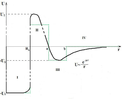
Figure 6: The approximation of rectangular well for potential of OHe-nucleus system.

Solutions of Schrodinger equation for each of the four regions, indicated on Fig. 6, are considered in Appendix. In the result of their sewing one obtains the condition for the existence of a low-energy level in OHe-nucleus system,

$$sin(k_{3}b+\delta)=\sqrt{\frac{1}{2mU_{3}}}\cdot k_{3},$$ (246)

where $k_{3}$ and $\delta$ are, respectively, the wave number and phase of the wave function in the region III (see Appendix for details).

With the use of the potential (245) in the Eq.(246), intersection of the two lines gives graphical solution presented on Fig. 7.

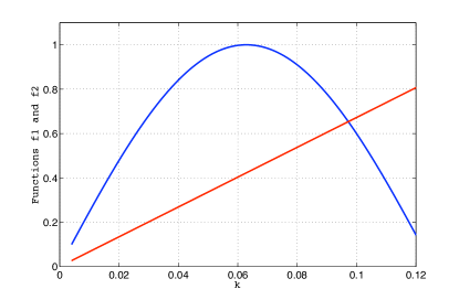
Figure 7: Graphical solution of transcendental equation.

Based on this solution one obtains from Eq.(261) the energy levels of a bound state in the considered potential well.

The energy of this bound state and its existence strongly depend on the parameters $\mu$ and $g^{2}$ of nuclear potential (243). On the Fig. 8 the region of these parameters, giving 2-6 keV energy level in OHe bound states with sodium and iodine are presented. In these calculations the mass of OHe was taken equal to $m_{o}=1TeV$.

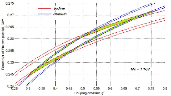
Figure 8: The region of parameters $\mu$ and $g^{2}$, for which Na and I have a level in the interval 2-6 keV. For each nucleus two narrow strips determine the region of parameters, at which the bound system of this element with OHe has a level in 2-6 keV energy range. The outer line of strip corresponds to the level of 6 keV and the internal line to the level of 2 keV. The region of intersection of strips correspond to existence of 2-6 keV levels in both OHe-Na and OHe-I systems, while the piece of strip between strips of other nucleus corresponds to the case, when OHe bound state with this nucleus has 2-6 keV level, while the binding energy of OHe with the other nuclei is less than 2 keV by absolute value.

The rate of radiative capture of OHe by nuclei should be accurately calculated with the use of exact form of wave functions, obtained for the OHe-nucleus bound state. This work is now in progress. One can use the analogy with the radiative capture of neutron by proton, considered in textbooks (see e.g. mkpa2LL4 ) with the following corrections:

• There is only E1 transition in the case of OHe capture.

• The reduced masses of n-p and OHe-nucleus systems are different

• The existence of dipole Coulomb barrier leads to a suppression of the cross section of OHe radiative capture.

With the account for these effects our first estimations give the rate of OHe radiative capture, reproducing the level of signal, detected by DAMA.

Formation of OHe-nucleus bound system leads to energy release of its binding energy, detected as ionization signal in DAMA experiment. In the context of our approach the existence of annual modulations of this signal in the range 2-6 keV and absence of such effect at energies above 6 keV means that binding energy of Na-OHe and I-OHe systems should not exceed 6 keV, being in the range 2-6 keV for at least one of these elements. These conditions were taken into account for determination of nuclear parameters, at which the result of DAMA can be reproduced. At these values of $\mu$ and $g^{2}$ energy of OHe binding with other nuclei can strongly differ from 2-6 keV. In particular, energy release at the formation of OHe bound state with thallium can be larger than 6 keV. However, taking into account that thallium content in DAMA detector is 3 orders of magnitude smaller, than NaI, such signal is to be below the experimental errors.

It should be noted that the results of DAMA experiment exhibit also absence of annual modulations at the energy of MeV-tens MeV. Energy release in this range should take place, if OHe-nucleus system comes to the deep level inside the nucleus (in the region I of Fig. 6). This transition implies tunneling through dipole Coulomb barrier and is suppressed below the experimental limits.

0.32.2 Energy levels in other nuclei

For the chosen range of nuclear parameters, reproducing the results of DAMA/ NaI and DAMA/LIBRA, we can calculate the binding energy of OHe-nucleus states in nuclei, corresponding to chemical composition of set-ups in other experiments. The results of such calculation for germanium, corresponding to the detector of CDMS experiment, are presented on Fig. 9.

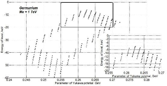
Figure 9: Energy levels in OHe bound system with germanium. The range of energies close to energy release in DAMA experiment is blown up to demonstrate that even in this range there is no formal intersection with DAMA results.

For all the parameters, reproducing results of DAMA experiment the predicted energy level of OHe-germanium bound state is beyond the range 2-6 keV, being dominantly in the range of tens - few-tens keV by absolute value. It makes elusive a possibility to test DAMA results by search for ionization signal in the same range 2-6 keV in other set-ups with content that differs from Na and I. In particular, our approach naturally predicts absence of ionization signal in the range 2-6 keV in accordance with the recent results of CDMS mkpa2Kamaev:2009gp .

We have also calculated the energies of bound states of OHe with xenon (Fig. 10), argon (Fig. 11), carbon (Fig. 12), aluminium (Fig. 13), fluorine (Fig. 14), chlorine (Fig. 15) and oxygen (Fig. 16).

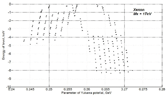
Figure 10: Energy levels in OHe bound system with xenon.

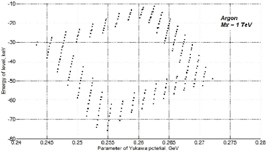
Figure 11: Energy levels in OHe bound system with argon.

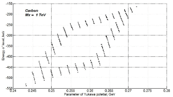
Figure 12: Energy levels in OHe bound system with carbon.

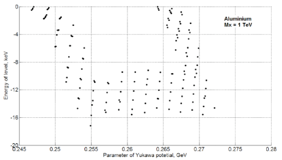
Figure 13: Energy levels in OHe bound system with aluminium.

Figure 14: Energy levels in OHe bound system with fluorine.

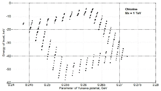
Figure 15: Energy levels in OHe bound system with chlorine.

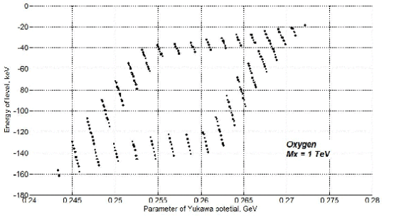
Figure 16: Energy levels in OHe bound system with oxygen.

0.32.3 Superheavy OHe

In view of possible applications for the approach, unifying spins and charges mkpa2Norma , we consider here the case of superheavy OHe, since the candidate for $X^{--}$, coming from stable 5th generation ($\bar{u}_{5}\bar{u}_{5}\bar{u}_{5}$) is probably much heavier, than 1 TeV. With the growth of the mass of O-helium the reduced mass (244) slightly grows, approaching with higher accuracy the mass of nucleus. It extends a bit the range of nuclear parameters $\mu$ and $g^{2}$, at which the binding energy of OHe with sodium and/or iodine is within the range 2-6 keV (see Fig. 17).

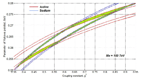
Figure 17: The range of parameters $\mu$ and $g^{2}$, for which Na and I have a level in the interval 2-6 keV for $S_{3}=100$. This range becomes a bit wider as compared with the case of $S_{3}=1$, presented on Fig. 8.

At these parameters the binding energy of O-helium with germanium and xenon are presented on figures 18 and 19, respectively. Qualitatively, these predictions are similar to the case of $S_{3}=1$. Though there appears a narrow window with OHe-Ge binding energy, below 6 keV for the dominant range of parameters energy release in CDMS is predicted to be of the order of few tens keV.

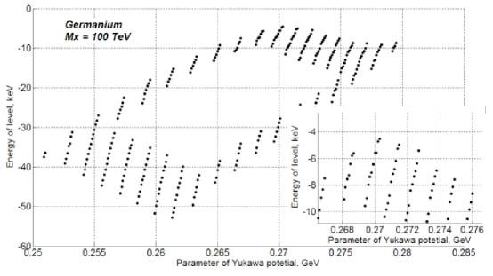
Figure 18: Energy levels in OHe bound system with germanium.

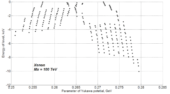
Figure 19: Energy levels in OHe bound system with xenon.

0.33 Conclusions

To conclude, the results of dark matter search in experiments DAMA/NaI and DAMA/LIBRA can be explained in the framework of composite dark matter scenario without contradiction with negative results of other groups. This scenario can be realized in different frameworks, in particular in Minimal Walking Technicolor model or in the approach unifying spin and charges and contains distinct features, by which the present explanation can be distinguished from other recent approaches to this problem mkpa2Edward (see also review and more references in mkpa2Gelmini ).

Our explanation is based on the mechanism of low energy binding of OHe with nuclei. We have found that within the uncertainty of nuclear physics parameters there exists a range at which OHe binding energy with sodium and/or iodine is in the interval 2-6 keV. Radiative capture of OHe to this bound state leads to the corresponding energy release observed as an ionization signal in DAMA detector.

OHe concentration in the matter of underground detectors is determined by the equilibrium between the incoming cosmic flux of OHe and diffusion towards the center of Earth. It is rapidly adjusted and follows the change in this flux with the relaxation time of few minutes. Therefore the rate of radiative capture of OHe should experience annual modulations reflected in annual modulations of the ionization signal from these reactions.

An inevitable consequence of the proposed explanation is appearance in the matter of DAMA/NaI or DAMA/LIBRA detector anomalous superheavy isotopes of sodium and/or iodine, having the mass roughly by $m_{o}$ larger, than ordinary isotopes of these elements. If the atoms of these anomalous isotopes are not completely ionized, their mobility is determined by atomic cross sections and becomes about 9 orders of magnitude smaller, than for O-helium. It provides their conservation in the matter of detector. Therefore mass-spectroscopic analysis of this matter can provide additional test for the O-helium nature of DAMA signal. Methods of such analysis should take into account the fragile nature of OHe-Na (and/or OHe-I) bound states. Their binding energy is only few keV.

With the account for high sensitivity of our results to the values of uncertain nuclear parameters and for the approximations, made in our calculations, the presented results can be considered only as an illustration of the possibility to explain puzzles of dark matter search in the framework of composite dark matter scenario. However, even at the present level of our studies we can make a conclusion that the ionization signal expected in detectors with the content, different from NaI, can be dominantly in the energy range beyond 2-6 keV. Therefore test of results of DAMA/NaI and DAMA/LIBRA experiments by other experimental groups can become a very nontrivial task.

0.34 Acknowledgments

We would like to thank Jean Pierre Gazeau for discussions.

Appendix. Solution of Schrodinger equation for rectangular well

In the 4 regions, indicated on Fig. 6, Schrodinger equation has the form

$$I:\frac{1}{r}\frac{d^{2}}{dr^{2}}(r\psi_{1})+k_{1}(r)^{2}\psi_{1}=0,k_{1}(r)=k_{1}=\sqrt{2m(U_{1}-|E|)};$$ (247)

$$II:\frac{1}{r}\frac{d^{2}}{dr^{2}}(r\psi_{2})+k_{2}(r)^{2}\psi_{2}=0,k_{2}(r)=k_{2}=\sqrt{2m(U_{2}-|E|)};$$ (248)

$$III:\frac{1}{r}\frac{d^{2}}{dr^{2}}(r\psi_{3})+k_{3}(r)^{2}\psi_{3}=0,k_{3}(r)=k_{3}=\sqrt{2m(U_{3}-|E|)};$$ (249)

$$IV:\frac{1}{r}\frac{d^{2}}{dr^{2}}(r\psi_{4})-k_{4}(r)^{2}\psi_{4}=0,k_{4}(r)=k_{4}=\sqrt{2m|E|}.$$ (250)

The wave functions in these regions with the account for the boundary conditions have the form mkpa2LL3

$$I:\psi_{1}=A\frac{\sin(k_{1}r)}{r};$$ (251)

$$II:\psi_{2}=\frac{B_{1}\cdot exp(-k_{2}r)+B_{2}\cdot exp(k_{2}r)}{r};$$ (252)

$$III:\psi_{3}=C\frac{\sin(k_{3}r+\delta)}{r}$$ (253)

$$IV:\psi_{4}=D\frac{\exp(-k_{4}r)}{r}$$ (254)

The conditions of continuity of a logarithmic derivative $\frac{\psi_{i}^{\prime}}{\psi_{i}}=\frac{\psi_{i+1}^{\prime}}{\psi_{i+1}}$ îò $\emph{r}\psi$ at the boundaries of these regions $r=R_{A}$, $r=a$ and $r=b$ are given by

$$I-II:k_{1}\cdot ctg(k_{1}R_{A})=k_{2}\cdot\frac{exp(k_{2}R_{A})-F\cdot exp(-k_{2}R_{A})}{exp(k_{2}R_{A})+F\cdot exp(-k_{2}R_{A})},$$ (255)

$$II-III:k_{3}\cdot ctg(k_{3}a+\delta)=k_{2}\cdot\frac{exp(k_{2}a)-F\cdot exp(-k_{2}a)}{exp(k_{2}a)+F\cdot exp(-k_{2}a)},$$ (256)

$$III-IV:k_{3}\cdot ctg(k_{3}b+\delta)=-k_{4},$$ (257)

where

$$F=B_{1}/B_{2}.$$ (258)

Now we can solve this system of equations for 3 variables. It follows from Eq. (255) that

$$F=exp(2k_{2}R_{A})\cdot\frac{k_{2}-k_{1}\cdot ctg(k_{1}R_{A})}{k_{2}+k_{1}\cdot ctg(k_{1}R_{A})},$$ (259)

and from Eq. (256)

$$\delta=-k_{3}a+arcctg(\frac{k_{2}}{k_{3}}\cdot\frac{exp(k_{2}a)-F\cdot exp(-k_{2}a)}{exp(k_{2}a)+F\cdot exp(-k_{2}a)}).$$ (260)

Since

$$E=U(r)-\frac{k^{2}}{2m},$$ (261)

one has

$$k_{4}=\sqrt{2mU-k_{3}^{2}},$$ (262)

Then Eq.(257) has the form

$$k_{3}^{2}[\frac{1}{sin^{2}(k_{3}b+\delta)}-1]=2mU_{3}-k_{3}^{2},$$ (263)

On the Possibilities and Impossibilities of Random Dynamics A. Kleppe

0.35 The notion of theory

The ambition of the physicist’s search for a ’theory of everything’ is to formulate an ultimate, finite theory. Many, probably most physicists, favour the Grand Unified Theory (GUT)-scenario, based on the assumption that the symmetry increases with energy (in the sense of larger symmetry groups describing the dynamics). The idea is that there is a large group at $10^{15}GeV$, which spontaneously breaks down and eventually ends up as SU(3)xSU(2)xU(1) at the weak scale. The interactions that are observed as separate, different forces at our energy level, are thus believed to be unified at GUT level. Physics itself seems to point towards unification and ”monocausality”, the amazing success of the Standard Model and electroweak unification indeed seems to whisper: ”Grand Unification”.

But there are alternative approaches according to which physics does not become simpler and more symmetric at higher energies, and there is no unification at higher energy.

The Random Dynamics project ak1RD is such an anti-grand-unification (AGUT) scheme, based on the assumption that the physical laws as we know them come about at low energy, from something un-describably complex that exists at high energy. The assumption is that at a fundamental scale, Nature is enormously complicated and most simply described in terms of randomness, and that the regular and fairly simple physics we observe comes about as one goes down from the high energy ”fundamental” level to our lower energy level. The idea is that any sufficiently complex and general model for the fundamental physics at (or above) the Planck scale, will in the low energy limit (where we operate) yield the physics we know. The reason is that as we go down the energy scale, the structure and complexity characteristic of the high energy level are shaved away. Only those features survive which are common for the long wavelength limit of any generic model of fundamental supra-Planck scale physics. The ambition of Random Dynamics is to ”derive” all the known physical laws as an almost unavoidable consequence of a random fundamental ”world machinery”.

When we call something fundamental, it’s usually implied that it is simple, but the ’simplicity’ of Random Dynamics lies in simple formulations like ”the fundamental world machinery is essentially random”. If one would be able to formulate the details of the ”laws”, they are probably exceedingly complicated!

The expectation that the fundamental level should be ’simple’ or ’transparent’ started with Euclid (300 B.C.), who found that he could bring back the theorems of geometry onto a small set of axioms. The basic idea is that the information content of a theory is contained in a finite set of axioms/principles/elements which so to speak constitutes the truth content of the theory.

In the beginning of the 20th century, David Hilbert wanted to do the same thing for mathematics, by constructing a formal axiomatic system from which he was going to derive all of mathematics.

In 1931, Kurt Gödel ak1Godel however proved that Hilbert’s program was impossible. He showed that any finite formal system of axioms is either incomplete or inconsistent. If you assume that your formal axiomatic system only tells the truth, it will not tell the whole truth, and if you assume that the axioms don’t allow to prove false theorems, there will be true theorems that cannot be proven within your axiomatic system. Gödel’s result concerns any formal axiomatic system. This is of course relevant for both mathematics and physics.

A physical theory is a mathematical description of some part of reality, allowing us to make accurate, verifiable predictions, and a ’fundamental physical theory’ is by definition a theory about the physics at very high energy $\sim$ Planck scale. But we of course don’t know anything about what happens at Planck scale, albeit we do know that physics looks very different at different energy levels. What is elementary at one level is complex at another level. For example in chemistry the atom is fundamental, while in particle physics it is complex and non-fundamental in the sense that given the equations of elementary particle physics, it is not obvious that atoms should be constructed as they are. It is thus very optimistic to believe that we can guess what physics is like at Planck scale.

But let us nevertheless imagine that such a fundamental theory is formulated: an equation, an algorithm or some principle(s) constituting the ultimate theory. According to Gödel, such a theory can however never encompass all of physics in a consistent way. There can exist excellent ’partial’ theories, Gödel doesn’t imply that there is no scientific truth or insight. But it’s not possible to formulate a theory that encompasses all of reality.

0.36 The information content of a theory

One way of dealing with the notion of theory, is to regard it as a (computer) program for predicting observations. Occam’s ”the simplest theory is best” then reads ”the most concise computer program is the best theory”.

Now, it’s very hard to make a theory about some part of reality - a ”system” - unless this system has some regularity. The reason is that a theory is a formulation of the information content of the system, and in a programming context, to fish out the information content of a system corresponds to compressing ak1Chaitin it. A very regular system obviously allows for more compression than a more chaotic system, so the computer program that describes a regular system is smaller than the program needed to describe a more chaotic system.

For example, a pattern like this:

has less complexity than this one:

Therefore, while we easily can formulate an algorithm P(A) which describes/generates the pattern ${\bf{A}}$, a description of ${\bf{B}}$ may require all the information in ${\bf{B}}$, unless we manage to find a way of compressing the pattern ${{\bf{B}}}$. We can conclude that most probably, $P(A)\leq P(B)$. Now, unless the amount of information of the theory is smaller than the amount of information of the the described system, the theory strictly speaking is no theory. In the pattern ${\bf{B}}$ above, there does not seem to be any clear regularity, thus no obvious compression is at hand, and there is no theory (or algorithm) for ${\bf{B}}$! But there might come a theory! The day someone finds a regularity in ${\bf{B}}$ that allows a algorithm generating ${\bf{B}}$ to be formulated, then we would have a theory for ${\bf{B}}$.

Suppose that you have a theory: a program withe fewer bits than the system described by the theory. It is good to have a theory, but you are very ambitious, and want to have a ”fundamental theory”, meaning the smallest theory that encompasses the (non-redundant) information of the described system.

In a computer context your ”system” can for example be a string of tokens like

$S_{1}$ = 1000110110101111100010… or

$S_{2}$ = ABCQQBCARQQAA.. or

$S_{3}$ = 1269789125482976502…

and your ”theory” is an algorithm that gives rise to your string. The fundamental theory for a string is the smallest program that generates this string, i.e. the program with the smallest complexity (i.e. the least information).

So you have a system (a string of numbers) $S$, and a small program $P_{S}$ which generates $S$. $P_{S}$ is rather small, so you may think that $P_{S}$ is your fundamental theory. But $P_{S}$ is perhaps still compressible - you just haven’t realized it. And still worse: if $P_{S}$ were incompressible, you would not be able to prove it, precisely because you can never prove that nobody will never find a program $P_{S}^{\prime}$ which is smaller than $P_{S}$, such that $P_{S}^{\prime}$ in its turn generates $P_{S}$: $P_{S}^{\prime}$ $\rightarrow$ $P_{S}$.

And since you cannot know if there is such a program $P_{S}^{\prime}$, you cannot decide on the complexity of $S$, because its complexity is defined as being equal to the complexity of the smallest program that generates $S$…

A ”fundamental theory” which describes $S$ would thus have the same complexity as $S$. But since you cannot ever prove that a program $P_{S}$ that generates $S$ is the smallest possible, the complexity of $S$ is undecidable. You may have a small program $P_{S}$ that generates $S$, but you cannot know if $P_{S}$ is the smallest program generating $S$, and therefore, you cannot know if a theory is fundamental or not. This is true in any situation where we want to formulate a theory about some part of the world or the entire world, in terms of a finite set of axioms.

An axiom is a statement or a string that we simply have to define as fundamental (meaning that it cannot be defined in terms of something more fundamental). And a pattern is random if it has no (obvious) pattern, i. e. there is no obvious plan behind its structure (so it cannot be defined by something even more fundamental). As we saw above, we cannot prove that any string is fundamental (incompressible), so we cannot prove that an axiom is fundamental. Likewise, we cannot prove that a random pattern is random, but we can with cetrainty claim that an axiom should be (information-theoretically) random.

In sum: the search for a theory of everything can be regarded as a quest for an ultimate compressions of the world. But since we cannot know when we have reached the limit of compressibility we can never know when or if our theory is a theory of everything, because we cannot:

- prove incompressibility.

- prove randomness.

- prove that some statement or string A is an axiom.

0.37 Random Dynamics

In Random Dynamics, the problems in formulating an ultimate theory are circumvened by not starting from a well-defined, finite set of formal axioms, but from ”a random mathematical structure” ${\cal{M}}$, which is not described in great detail. All we know is that the fundamental ”world machinery” ${\cal{M}}$ is a very general, random mathematical structure, which contains non-identical elements and some set-theoretical notions. There are also strong exchange forces present, but there is as yet no physics. At some stage ${\cal{M}}$ comes about, and then physics follows.

We have no detailed information about the nature of the elements of ${\cal{M}}$, but we nevertheless claim that the observed physics emerges from ${\cal{M}}$, defined as a generic set randomly chosen from a set of such sets, {${\cal{M}}_{1}$, ${\cal{M}}_{2}$, ${\cal{M}}_{3}$..} where every ${\cal{M}}_{j}$ gives rise to the known physics at low energy, and none of the ${\cal{M}}_{j}$ is known in elaborate detail.

While Random Dynamics avoids the consistency and completeness problems of a formal ultimate theory by describing its basic assumptions in heuristic, non-formal terms, there is still something worrisome about this approach. The problem is the apparent paradox that we start with something which by definition is generic and not described in great detail. How can we ascribe properties - and such powerful properties - to something that not observable or even describable?

Should we not demand that ${\cal{M}}$ be related it to something more substantial and well-known? The claim is after all that ${\cal{M}}$ underlies all of reality.

0.38 An excursion into the real

So let us consider something very well known: the real numbers, ${\bf{\cal{R}}}$. A real number can be described as a length measured with arbitrary precision with up to an infinite number of digits, and a computable real number is a number for which there is a computer program that calculates its digits one by one.

Next consider the set of all possible computer programs, which is a countable set. We list the possible computer programs:

$${\hskip 142.26378pt}P_{1}$$

$${\hskip 142.26378pt}P_{2}$$

$${\hskip 142.26378pt}P_{3}$$

$${\hskip 142.26378pt}...$$

Since each computable real corresponds to a computer program, the set of computable reals is also countable.

But the set of all real numbers ${\cal{R}}$ has the power of the continuum, so ${\cal{R}}$ is uncountable, and thus the set of uncomputable reals, i. e. [${\cal{R}}$ $\backslash$ {computable reals}] is uncountable. And there are many more uncomputable reals than computable reals, so if you randomly pick a real number from the number line, the number you pick will with probability 1 be an uncomputable number!

Proof: take all computable reals, take all computer programs that compute these reals, and make a list:

$$p_{1} \sim first{\hskip 5.69054pt}computable{\hskip 5.69054pt}real{\hskip 5.69054pt}r_{1}$$

$$p_{2} \sim second{\hskip 5.69054pt}computable{\hskip 5.69054pt}real{\hskip 5.69054pt}r_{2}$$

$$p_{3} \sim third{\hskip 5.69054pt}computable{\hskip 5.69054pt}real{\hskip 5.69054pt}r_{3}$$

$$....$$

$$p_{k} \sim kth{\hskip 5.69054pt}computable{\hskip 5.69054pt}real{\hskip 5.69054pt}r_{k}$$

$$....$$

and cover each $r_{j}$ with the interval $\epsilon/2^{j}$. The size of the sum of all the covering intervals is then $\epsilon/2+\epsilon/2^{2}+\epsilon/2^{3}+...\epsilon/2^{k}+..=\epsilon$, where $\epsilon$ can be made indefinitely small. The probability of randomly picking a computable real from the number line is thus indefinitely small - i.e. zero. Thus:

The set of reals that can be individually named or specified or even defined or referred to within formal language, has probability zero. Thus:

Reals are un-nameable with probability 1.

Even if we in practice talk about these un-nameable reals, only those reals that are defined by a finite amount of information can be spoken about on a formally secure ground. We can refer to the uncomputable reals, but we can by definition not specify the properties of an individual uncomputable real.

So, when we talk about ’the real numbers’, we talk about entities that we mostly cannot label individually. Only very few of them are tangible, computable, most of them are untouchable, un-nameable. Among these un-nameable reals we discern the random reals, which are maximally incompressible reals, meaning that few or none of the digits are computable by a program.

So the few reals that are hands-on are those that are completely defined by a finite number of digits in the sense that there is a finite number of well-defined programs by which the digits can be calculated.

But as we know, that doesn’t make the notion of real numbers useless, on the contrary. The same is true for ${\cal{M}}$. We don’t know its details, but we are nevertheless able to deduce a wealth of information from the assumption of its existence.

0.39 Emergent phenomena

The requirement that a fundamental theory should consist of a finite set of simple elements from which the observed physics can be deduced, means that the ”fundamental” is supposed to be finite, transparent and handable.

According to the Random Dynamics approach there is however no such transparency at the fundamental level, which on the contrary is believed to be characterized by a lack of (visible) organized structure. Only the initial input can be perceived as simple and transparent, consisting of the set ${\cal{M}}$, some set theoretical notions and some exchange forces, from which the physics emerges.

Emergence is a process reconstructing a system in such a way that some new - emergent - properties appear.

An example is deterministic chaos, where deterministic equations of motion lead to apparently unpredictable behaviour.

The randomness originates from a situation where the effective dynamic which maps initial conditions to states at later times, becomes so complicated that an observer has no way to compute precisely enough to predict the future behaviour.

Opposite example: order arising from disorder, like in self-avoiding random walk in 2 dimensions, where the step-by-step behaviour of a particle is constrained by the demand that the next step is taken in a random direction, with the exclusion of the direction from which it comes. This results in a path tracing out a self-similar set of positions in the plane: a ”fractal” structure emerges!

Deterministic chaos and self-avoiding random walk are examples of emergence of pattern. The emerging features are new and in direct opposition to the system’s defining character.

Emergent phenomena also have to do with scale. The system as a whole may have properties that are not apparent at elementary levels of scale; the same goes for energy levels.

An emergent property which is well-defined at one level may be meaningless at another. For example: the Möbius strip. The strip may be cut up in smaller parts, each of which is orientable; while the entire Möbius strip is not. The non-orientability can be described as emerging while perceiving the strip, i. e. the sum of the parts, as a whole. According to the philosophy of emergence, while there certainly exist certain global, fundamental principles, many of the notions we perceive as fundamental are only ”locally fundamental”.

In condensed matter physics we see many instances of emergence, and while investigating whether physics follows a GUT or an anti-GUT scheme, it can be useful to use analogy, by comparing high energy physics with the physics of quantum liquids, superconductors, superfluids, ferromagnets. Condensed matter systems display many properties reminiscent of high energy physics, both ”GUT-features” and ”AGUT-features” ak1Volovik .

Superfluid ${}^{3}He-A$ is an example of this; at high temperatures, the ${}^{3}He$ gas, and at lower temperatures the ${}^{3}He$ liquid have all the symmetries of ordinary condensed matter: translational invariance, global U(1) group, etc. When the temperature goes down, the liquid ${}^{3}He$ reaches the superfluid temperature $T_{c}\sim 1mK$, and below $T_{c}$ all the symmetries disappear, except translational invariance: ${}^{3}He$ is still liquid. This low energy symmetry breaking resembles the one in particle physics - in accordance with the GUT scenario. But then, as $T_{c}\rightarrow 0$, the superfluid ${}^{3}He-A$ gradually acquires all the high energy symmetries. From nothing it gets Lorenz invariance, local gauge invariance, etc, in a perfect AGUT spirit.

Seemingly fundamental features may thus disappear or emerge with changing energy or scale, it is thus very hard to establish what is ”fundamental” - hard to formulate an ultimate theory. Some things that are scale invariant however remain:

- physical principles (like the principle of least action, conservation of energy).

- mathematical rules (integers, mathematical operations, logic).

0.40 Conclusion

The goal of the Random Dynamics project is to formulate the minimal set of assumptions needed for deriving the laws of nature, and thereafter derive the known physics. It may seem both too vague and to technical, but the notion of a set as general as the Random Dynamics fundamental ”world machinery” ${\cal{M}}$ is not more empty or meaningless than the notion of real numbers.

The stumbling block of any ultimate theory, is its all-encompassing ambition. An ultimate theory is supposed to be finite, containing a finite amount of information (axioms, assumptions), but since a finite formal system of axioms is either incomplete or inconsistent, no finite theory can ever be ”ultimate” in the sense of all-explanatory. The Random Dynamics random point of departure offers a way out of this dilemma.

The Random Dynamics philosphy that symmetries and seemingly fundamental laws of nature are in reality emergent phenomena, is moreover supported by data from condensed matter physics.

Spin Connection Makes Massless Spinor Chirally Coupled to Kaluza-Klein Gauge Field After Compactification of $M^{1+5}$ to $M^{1+3}\times$ Infinite Disc Curved on $S^{2}$ D. Lukman¹, N. S. Mankoč Borštnik¹ and H. B. Nielsen²

0.41 Introduction

The idea of Kaluza and Klein of obtaining the electromagnetism - and under the influence of their idea in now a days also the weak and colour fields - from purely gravitational degrees of freedom connected with having extra dimensions is very elegant, but were almost killed by a ”no-go theorem” of E. Witten dhn1witten telling that these kinds of theories have very severe difficulties with obtaining massless fermions chirally coupled to the Kaluza-Klein-type gauge fields in $d=1+3$, as required by the standard model of the electroweak and colour interactions. There may be escapes from the ”no-go theorem” by having torsion or by having an orbifold structure in the extra dimensional space. In refs. dhn1hnkk06 ; dhn1hn07 we achieved masslessness of spinors with the appropriate choice of a boundary on a finite disc.

When we have no fermions present and only the curvature in the Lagrange density the spin connections are determined from the vielbein fields and the torsion is zero. A major point of the present article is that in some cases the spin connections, we call these cases ”an effective two-dimensionality” is not fully determined from the vielbeins. In such special cases there is the possibility of having torsion in a gauge theory of gravity with spin connections and vielbeins and therefore for a possibility for a Kaluza-Klein-like model, which effectively in four dimensional space-time manifests the known gauge fields, while yet the Lagrange density contains only the curvature. This opens a loop hole through the Witten’s ”no-go theorem” even if there are no boundaries, which take care of maslesness dhn1hnkk06 ; dhn1hn07 .

In the here proposed types of models is the chance for having chirally mass protected fermions in a theory in which the chirally protecting effective four dimensional gauge fields are true Kaluza-Klein-like fields the degrees of which inherit from the higher dimensional gravitational ones. We are thus hoping for a revival of true Kaluza-Klein[like models as candidates for phenomenological viable models!

One of us has been trying for long to develop the Approach unifying spins and charges so that spinors which carry in $d\geq 4$ nothing but two kinds of the spin (no charges), would manifest in $d=(1+3)$ all the properties assumed by the Standard model. The Approach proposes in $d=(1+(d-1))$ a simple starting action for spinors with the two kinds of the spin generators ($\gamma$ matrices): the Dirac one, which takes care of the spin and the charges, and the second one, anticommuting with the Dirac one, which generates families . A spinor couples in $d=1+13$ to only the vielbeins and (through two kinds of the spin generators to) the spin connection fields. Appropriate breaks of the starting symmetry lead to the left handed quarks and leptons in $d=(1+3)$, which carry the weak charge while the right handed ones are weak chargeless. The Approach might have the right answer to the questions about the origin of families of quarks and leptons, about the explicit values of their masses and mixing matrices as well as about the masses of the scalar and the weak gauge fields, about the dark matter candidates, and about the breaking of the discrete symmetries.

Let us point out that in odd dimensional spaces and in even dimensional spaces devisible with four there is no mass protection in the Kaluza-Klein-like theories dhn1hn06 . The spaces therefore, for which we can have a hope that the Kaluza-Klein-like theories lead to chirally protected fermions and accordingly to the effective theory of the standard model of the electroweak and colour interactions, have $2(2n+1)$ dimensions.

Let us accordingly assume that we start with the $2(2n+1)$-dimensional space, with gravity only, described by the action

$${\cal S}=\alpha\int\;d^{d}x\,E{\cal\,R}.$$ (264)

with the Riemann scalar ${\cal R}={\cal R}_{abcd}\eta^{ac}\eta^{bd}$ determined by the Riemann tensor

$${\cal R}_{abcd}=f^{\alpha}{}_{[a}f^{\beta}{}_{b]}(\omega_{cd\beta,\alpha}-\omega_{ce\alpha}\omega^{e}{}_{d\beta}),$$ (265)

with vielbeins $f^{\alpha}{\!}_{a}$ (the choice of the meaning of indices can be found in the footnote  ), the gauge fields of the infinitesimal generators of translation, and spin connections $\omega_{ab\alpha}$ the gauge fields of the $S^{ab}=\frac{i}{4}(\gamma^{a}\gamma^{b}-\gamma^{b}\gamma^{a})$. $[a\,\,b]$ means that the antisymmetrization must be performed over the two indices $a$ and $b$.

In the ref. dhn1dhnproc04 we proved that in the absent of the fermion fields the action in Eq.( 264 leads to the equations of motion (Eq. (6.10) in the ref. dhn1dhnproc04 )

$$(d-2)\,\omega_{b}{}^{c}{}_{c}=\frac{e^{a}{}_{\alpha}}{E}\partial_{\beta}\left(Ef^{\alpha}{}_{[a}f^{\beta}{}_{b]}\right),$$ (266)

which for $d=2$ clearly demonstrates that any spin connection $\omega_{b}{}^{c}{}_{c}=f^{\alpha}{}_{d}\omega_{b}{}^{d}{}_{c}$ (which can in $d=2$ have only two different indices) satisfies this equation. In the same ref. dhn1dhnproc04 , Eq.(6.15), we also prove that for $d=2$ any zweibein fulfills the equations of motion

$$Ef^{\alpha}{}_{[a}f^{\beta}{}_{b]} = \frac{1}{4}\varepsilon^{\alpha\beta}\varepsilon_{ab}.$$ (267)

It also can be shown (dhn1dhnproc04 , Eq.(6.17)) that the variation of the action (264) with respect to vielbeins leads to the equation

$$-e^{s}{}_{\sigma}R+4f^{\tau t}\omega_{st\sigma,\tau}=0,$$ (268)

which is trivially zero for any $R$. This can be seen by multiplying the above equation by $f^{\sigma}{}_{s}$ and summing over the two indices $\sigma$ and $s$. It follows then that $(d-2)R=0.$

We shall accordingly make a choice for $d=2$ of a zweibein, which curves an infinite disc (a two dimensional infinite plane with the rotational symmetry around the axes perpendicular to the plane) into a spehere $S^{2}$ with the radius $\rho_{0}$

$$e^{s}{}_{\sigma}=f^{-1}\begin{pmatrix}1&0\\ 0&1\end{pmatrix},f^{\sigma}{}_{s}=f\begin{pmatrix}1&0\\ 0&1\end{pmatrix},$$ (269)

with

$$f = 1+(\frac{\rho}{2\rho_{0}})^{2}=\frac{2}{1+\cos\vartheta},$$

$$x^{5} = \rho\,\cos\phi,\quad x^{6}=\rho\,\sin\phi,\quad E=f^{-2}.$$ (270)

The angle $\vartheta$ is the ordinary asimutal angle on a sphere. The last relation follows from $ds^{2}=e_{s\sigma}e^{s}{}_{\tau}dx^{\sigma}dx^{\tau}=f^{-2}(d\rho^{2}+\rho^{2}d\phi^{2})$. We use indices $s,t=5,6$ to describe the flat index in the space of an infinite plane, and $\sigma,\tau=(5),(6),$ to describe the Einstein index. $\phi$ determines the angle of rotations around the axis through the two poles of a sphere, while $\rho=2\rho_{0}\,\sqrt{\frac{1-\cos\vartheta}{1+\cos\vartheta}}$, where $\tan\frac{\vartheta}{2}=\frac{\rho}{2\rho_{0}}$. Fig.( 20) shows the (well known) relation between $\rho$ and $\vartheta$.

Figure 20: The disc is curved on the sphere $S^{2}$.

We make a choice of the spin connection field

$$f^{\sigma}{}_{s^{\prime}}\,\omega_{st\sigma} =iF\,f\,\varepsilon_{st}\;\frac{e_{s^{\prime}\sigma}x^{\sigma}}{(\rho_{0})^{2}}=i\varepsilon_{st}\,\frac{F\,\sin\vartheta}{\rho_{0}}\,(\cos\phi,\sin\phi),\quad s=5,6,\,\,\;\sigma=(5),(6),$$ (271)

which for the choice $0<2F\leq 1$ allows only one massless spinor of a particular charge on such $S^{2}$, as we shall see in sect. 0.42.

Accordingly, if we have a Weyl spinor in $d=(1+5)$, which breaks into $M^{1+3}$ cross an infinite disc, which by a zweibein is curved on $S^{2}$, then at least for this case we know the solutions for the gauge fields fulfilling the equations of motion for the action linear in the curvature, where the vielbein and spin connection guarantee masslessness of spinors in the space $d=1+3$.

Let us point out that the two dimensionality can be simulated in any dimension larger than two, if vielbeins and spin connections are completely flat in all but two dimensions.

We take (in this paper we do not study the appearance of families, as we also did not in the refs. dhn1hnkk06 ; dhn1hn07 ) for the covariant momentum of a spinor

$$p_{0a} = f^{\alpha}{\!}_{a}p_{0\alpha},\quad p_{0\alpha}\psi=p_{\alpha}-\frac{1}{2}S^{cd}\omega_{cd\alpha}$$

$$a = 0,1,2,3,5,\cdots d,\quad\alpha=(0),(1),(2),(3),(5),\cdots(d),.$$ (272)

A spinor carries in $d\geq 4$ nothing but a spin and interacts accordingly with only the gauge fields of the corresponding generators of the infinitesimal transformations (of translations and the Lorentz transformations in the space of spinors), that is with vielbeins $f^{\alpha}{\!}_{a}$ and spin connections $\omega_{ab\alpha}$.

The corresponding Lagrange density for a Weyl spinor has the form ${\cal L}_{W}=\frac{1}{2}[(\psi^{\dagger}E\gamma^{0}\gamma^{a}p_{0a}\psi)+(\psi^{\dagger}E\gamma^{0}\gamma^{a}p_{0a}\psi)^{\dagger}]$, leading to the equation of motion

$${\cal L}_{W} = \psi\,\gamma^{0}\gamma^{a}E\{f^{\alpha}{}_{a}p_{\alpha}+\frac{1}{2E}\{p_{\alpha},f^{\alpha}{}_{a}E\}_{-}-\frac{1}{2}S^{cd}\omega_{cda}\}\psi=0,$$ (273)

with $E=\det(e^{a}{\!}_{\alpha}),$ where

$$\omega_{cda} = \Re e\;\omega_{cda},\;\;{\rm if\;\;c,d,a\;\;all\;\;different}$$ (274)

$$= i\,\Im m\;\omega_{cda},\;\;\rm{otherwise}.$$

Let us have no gravity in $d=(1+3)$ ($f^{\mu}{}_{m}=\delta^{\mu}_{m}$ and $\omega_{mn\mu}=0$ for $m,n=0,1,2,3,\mu=0,1,2,3$) and let us make a choice of a zweibein and spin connection on our disc as written in Eqs. (0.41,271). ($S^{2}$ does not break the rotational symmetry on the disc, it breaks the translational symmetry after making a choice of the nothern ans southern pole.)

Although for any $0<2F\leq 1$ only one massless spinor on $S^{2}$ is allowed, it will be demonstrated that in the particular case that $2F=1$ the spin connection term $-S^{56}\omega_{56\sigma}$ compensates the term $\frac{1}{2Ef}\{p_{\sigma},Ef\}_{-}$ for the left handed spinor with respect to $d=1+3$, while for the spinor of the opposite handedness the spin connection term doubles the term $\frac{1}{2Ef}\{p_{\sigma},Ef\}_{-}$.

The vielbeins and spin connection fields of Eqs. (0.41,271) are invariant under the rotation around the north pole to south pole axis of the $S^{2}$ sphere. The infinitesimal coordinate transformations manifesting this symmetry are: $x^{{}^{\prime}\mu}=x^{\mu},$ $x^{{}^{\prime}\sigma}=x^{\sigma}+\phi_{A}\,K^{A\sigma}$, with $\phi_{A}$ the parameter of rotations around the axis which goes through both poles and with the infinitesimal generators of rotations around this axis $M^{(5)(6)}(=x^{(5)}p^{(6)}-x^{(6)}p^{(5)}+S^{(5)(6)})$

$$K^{A\sigma}=K^{(56)\sigma}=-iM^{(5)(6)}x^{\sigma}=\varepsilon^{\sigma}{}_{\tau}x^{\tau},$$ (275)

with $\varepsilon^{\sigma}{}_{\tau}=-1=-\varepsilon_{\tau}{}^{\sigma},\,\varepsilon^{(5)(6)}=1.$ The operators $K^{A}_{\sigma}=f^{-2}\varepsilon_{\sigma\tau}x^{\tau}$ fulfil the Killing relation

$$K^{A}_{\sigma,\tau}+\Gamma^{\sigma^{\prime}}{}_{\sigma\tau}K^{A}_{\sigma^{\prime}}+K^{A}_{\tau,\sigma}+\Gamma^{\sigma^{\prime}}{}_{\tau\sigma}K^{A}_{\sigma^{\prime}}=0,$$

(with $\Gamma^{\sigma^{\prime}}{}_{\sigma\tau}=-\frac{1}{2}\,g^{\rho\sigma^{\prime}}(g_{\tau\rho,\sigma}+g_{\sigma\rho,\tau}-g_{\sigma\tau,\rho})$).

The equations of motion for spinors (the Weyl equations) which follow from the Lagrange density (Eq. 273) are then

$$\{E\gamma^{0}\gamma^{m}p_{m}+Ef\gamma^{0}\gamma^{s}\delta^{\sigma}_{s}(p_{0\sigma}+\frac{1}{2Ef}\{p_{\sigma},Ef\}_{-})\}\psi=0,\quad{\rm with}$$

$$p_{0\sigma}=p_{\sigma}-\frac{1}{2}S^{st}\omega_{st\sigma},$$ (276)

with $f$ from Eq. (0.41) and with $\omega_{st\sigma}$ from Eq. (271). From $\gamma^{a}p_{0a}\gamma^{b}p_{0b}=p_{0a}p_{0}{}^{a}-iS^{ab}S^{cd}\,{\cal R}_{abcd}+S^{ab}\,{\cal T}^{\beta}{}_{ab}\,p_{0\beta}$ we find for the Riemann tensor of Eq. (265) and the torsion

$${\cal T}^{\beta}{}_{ab} = f^{\alpha}{}_{[a}(f^{\beta}{}_{b]})_{,\alpha}+\omega_{[a}{}^{c}{}_{b]}f^{\beta}_{c}.$$ (277)

From Eq. (265) we read that to the torsion on $S^{2}$ both, the zweibein $f^{\sigma}_{\tau}$ and the spin connection $\omega_{st\sigma}$, contribute. While we have on $S^{2}$ for ${\cal R}_{\sigma\tau}=f^{-2}\eta_{\sigma\tau}\frac{1}{\rho^{2}}$ and correspondingly for the curvature ${\cal R}=\frac{-2}{(\rho_{0})^{2}}$, we find for the torsion ${\cal T}^{s}{}_{ts^{\prime}}={\cal T}^{s}{}_{t\sigma}f^{\sigma}_{s^{\prime}}$ with ${\cal T}^{5}{}_{ss}=0={\cal T}^{6}{}_{ss},\quad s=5,6,$ ${\cal T}^{5}{}_{65}=-{\cal T}^{5}{}_{56}=-(f_{,6}+\frac{4iF(f-1)}{\rho^{2}}x_{5}),$ ${\cal T}^{6}{}_{56}=-{\cal T}^{6}{}_{65}=-f_{,5}+\frac{4iF(f-1)}{\rho^{2}}x_{6}.$ The torsion ${\cal T}^{2}={\cal T}^{s}{}_{ts^{\prime}}{\cal T}_{s}{}^{ts^{\prime}}$ is for our particular choice of the zweibein and spin connection fields from Eqs. (0.41,271) correspondingly equal to $-\frac{2\rho^{2}}{(\rho_{0})^{4}}(1-(2F)^{2})$. If we take the model dhn1mil with ${\cal T}^{2}={\cal T}^{s}{}_{ts^{\prime}}{\cal T}_{s}{}^{ts^{\prime}}+2{\cal T}^{s}{}_{ts^{\prime}}{\cal T}^{t}{}_{s}{}^{s^{\prime}}-4{\cal T}^{s}{}_{ts}{\cal T}_{s^{\prime}}{}^{ts^{\prime}}$, we obtain for the choice of fields from Eqs. (0.41,271) $\;\;{\cal T}^{2}=0$.

0.42 Equations of motion for spinors and the solutions

Let the spinor ”feel” the zweibein $f^{\sigma}{\!}_{s}=\delta^{\sigma}{\!}_{s}f(\rho),\,f(\rho)=1+(\frac{\rho}{2\rho_{0}})^{2}=\frac{2}{1+\cos\vartheta}$ and the spin connection $\omega_{st\sigma}=iF\varepsilon_{st}\frac{x_{\sigma}}{f\,\rho^{2}_{0}}\,=iF\frac{\sin\vartheta}{\rho_{0}}\,(\cos\phi,\sin\phi)$. The solution of the equations of motion (276) for a spinor in $(1+5)$-dimensional space, which breaks into $M^{(1+3)}$ $\times S^{2}$, should be written as a superposition of all four ($2^{6/2-1}$) states of a single Weyl representation. (We kindly ask the reader to see the technical details about how to write a Weyl representation in terms of the Clifford algebra objects after making a choice of the Cartan subalgebra, for which we take: $S^{03},S^{12},S^{56}$ in the refs. dhn1holgernorma2002 ; dhn1hn07 .) In our technique dhn1holgernorma2002 one spinor representation—the four states, which all are the eigenstates of the chosen Cartan subalgebra with the eigenvalues $\frac{k}{2}$, correspondingly—are the following four products of projections $\stackrel{{\scriptstyle ab}}{{[k]}}$ and nilpotents $\stackrel{{\scriptstyle ab}}{{(k)}}$:

$$\varphi^{1}_{1} = \stackrel{{\scriptstyle 56}}{{(+)}}\stackrel{{\scriptstyle 03}}{{(+i)}}\stackrel{{\scriptstyle 12}}{{(+)}}\psi_{0},$$

$$\varphi^{1}_{2} = \stackrel{{\scriptstyle 56}}{{(+)}}\stackrel{{\scriptstyle 03}}{{[-i]}}\stackrel{{\scriptstyle 12}}{{[-]}}\psi_{0},$$

$$\varphi^{2}_{1} = \stackrel{{\scriptstyle 56}}{{[-]}}\stackrel{{\scriptstyle 03}}{{[-i]}}\stackrel{{\scriptstyle 12}}{{(+)}}\psi_{0},$$

$$\varphi^{2}_{2} = \stackrel{{\scriptstyle 56}}{{[-]}}\stackrel{{\scriptstyle 03}}{{(+i)}}\stackrel{{\scriptstyle 12}}{{[-]}}\psi_{0},$$ (278)

where $\psi_{0}$ is a vacuum state for the spinor state. If we write the operators of handedness in $d=(1+5)$ as $\Gamma^{(1+5)}=\gamma^{0}\gamma^{1}\gamma^{2}\gamma^{3}\gamma^{5}\gamma^{6}$ ($=2^{3}iS^{03}S^{12}S^{56}$), in $d=(1+3)$ as $\Gamma^{(1+3)}=-i\gamma^{0}\gamma^{1}\gamma^{2}\gamma^{3}$ ($=2^{2}iS^{03}S^{12}$) and in the two dimensional space as $\Gamma^{(2)}=i\gamma^{5}\gamma^{6}$ ($=2S^{56}$), we find that all four states are left handed with respect to $\Gamma^{(1+5)}$, with the eigenvalue $-1$, the first two states are right handed and the second two states are left handed with respect to $\Gamma^{(2)}$, with the eigenvalues $1$ and $-1$, respectively, while the first two are left handed and the second two right handed with respect to $\Gamma^{(1+3)}$ with the eigenvalues $-1$ and $1$, respectively. Taking into account Eq. (278) we may write dhn1hn07 the most general wave function $\psi^{(6)}$ obeying Eq. (276) in $d=(1+5)$ as

$$\psi^{(6)}={\cal A}\,{\stackrel{{\scriptstyle 56}}{{(+)}}}\,\psi^{(4)}_{(+)}+{\cal B}\,{\stackrel{{\scriptstyle 56}}{{[-]}}}\,\psi^{(4)}_{(-)},$$ (279)

where ${\cal A}$ and ${\cal B}$ depend on $x^{\sigma}$, while $\psi^{(4)}_{(+)}$ and $\psi^{(4)}_{(-)}$ determine the spin and the coordinate dependent parts of the wave function $\psi^{(6)}$ in $d=(1+3)$

$$\psi^{(4)}_{(+)} = \alpha_{+}\;{\stackrel{{\scriptstyle 03}}{{(+i)}}}\,{\stackrel{{\scriptstyle 12}}{{(+)}}}+\beta_{+}\;{\stackrel{{\scriptstyle 03}}{{[-i]}}}\,{\stackrel{{\scriptstyle 12}}{{[-]}}},$$

$$\psi^{(4)}_{(-)} = \alpha_{-}\;{\stackrel{{\scriptstyle 03}}{{[-i]}}}\,{\stackrel{{\scriptstyle 12}}{{(+)}}}+\beta_{-}\;{\stackrel{{\scriptstyle 03}}{{(+i)}}}\,{\stackrel{{\scriptstyle 12}}{{[-]}}}.$$ (280)

Using $\psi^{(6)}$ in Eq. (276) and separating dynamics in $1+3$ and on $S^{2}$, the following relations follow, from which we recognize the mass term $m$: $\frac{\alpha_{+}}{\alpha_{-}}(p^{0}-p^{3})-\frac{\beta_{+}}{\alpha_{-}}(p^{1}-ip^{2})=m,$ $\frac{\beta_{+}}{\beta_{-}}(p^{0}+p^{3})-\frac{\alpha_{+}}{\beta_{-}}(p^{1}+ip^{2})=m,$ $\frac{\alpha_{-}}{\alpha_{+}}(p^{0}+p^{3})+\frac{\beta_{-}}{\alpha_{+}}(p^{1}-ip^{2})=m,$ $\frac{\beta_{-}}{\beta_{+}}(p^{0}-p^{3})+\frac{\alpha_{-}}{\beta_{+}}(p^{1}-ip^{2})=m.$ (One notices that for massless solutions ($m=0$) $\psi^{(4)}_{(+)}$ and $\psi^{(4)}_{(-)}$ decouple.) Taking into account that $S^{56}\stackrel{{\scriptstyle 56}}{{(+)}}=\frac{1}{2}\stackrel{{\scriptstyle 56}}{{(+)}}$, while $S^{56}\stackrel{{\scriptstyle 56}}{{[-]}}=-\frac{1}{2}\stackrel{{\scriptstyle 56}}{{[-]}}$, we end up with the equations of motion for ${\cal A}$ and ${\cal B}$ as follows

$$-2i\,f\,(\frac{\partial}{\partial z}+\frac{\partial\ln\sqrt{Ef}}{\partial z}-\frac{e^{-i\phi}}{\rho}G)\,{\cal B}+m\;{\cal A}=0,$$

$$-2i\,f\,(\frac{\partial}{\partial\bar{z}}+\frac{\partial\ln\sqrt{Ef}}{\partial\bar{z}}+\frac{e^{i\phi}}{\rho}G)\,{\cal A}+m\;{\cal B}=0,$$ (281)

where $z:=x^{5}+ix^{6}=\rho\,e^{i\phi}$, $\bar{z}:=x^{5}-ix^{6}=\rho\,e^{-i\phi}$ and $\frac{\partial}{\partial z}=\frac{1}{2}\,(\frac{\partial}{\partial x^{5}}-i\frac{\partial}{\partial x^{6}})=\frac{e^{-i\phi}}{2}\;(\frac{\partial}{\partial\rho}-\frac{i}{\rho}\,\frac{\partial}{\partial\phi})$, $\frac{\partial}{\partial\bar{z}}=\frac{1}{2}\,(\frac{\partial}{\partial x^{5}}+i\frac{\partial}{\partial x^{6}})=\frac{e^{i\phi}}{2}\;(\frac{\partial}{\partial\rho}+\frac{i}{\rho}\,\frac{\partial}{\partial\phi})$. Eq. (281) can be rewritten as follows

$$-if\,e^{-i\phi}\,(\frac{\partial}{\partial\rho}-\frac{i}{\rho}\,(\frac{\partial}{\partial\phi}-i2G)+\frac{\partial}{\partial\rho}\ln{\sqrt{Ef}}){\cal B}+m{\cal A}=0,$$

$$-if\,e^{i\phi}\,(\frac{\partial}{\partial\rho}+\frac{i}{\rho}\,(\frac{\partial}{\partial\phi}-i2G)+\frac{\partial}{\partial\rho}\ln{\sqrt{Ef}}){\cal A}+m{\cal B}=0,$$ (282)

with $G=F\frac{f-1}{f}(=\frac{1}{2}\,F(1-\cos\vartheta))$. Having the rotational symmetry around the axis perpendicular to the plane of the fifth and the sixth dimension we require that $\psi^{(6)}$ is the eigenfunction of the total angular momentum operator $M^{56}$

$$M^{56}\psi^{(6)}=(n+\frac{1}{2})\,\psi^{(6)},\quad M^{56}=x^{5}p^{6}-x^{6}p^{5}+S^{56}.$$ (283)

Let ${\cal A}={\cal A}_{n}(\rho)\,\rho^{n}\,e^{in\phi}$ and ${\cal B}={\cal B}_{n}(\rho)\,\rho^{-n}\,e^{in\phi}$.

Let us treat first the massless case ($m=0$). Taking into account that $\frac{G}{\rho}=\frac{\partial}{\partial\rho}\ln f^{\frac{F}{2}}$ and that $E=f^{-2}$ it follows

$$\frac{\partial\,\ln({\cal B}\,f^{-F-1/2})}{\partial\rho}=0,\qquad\frac{\partial\,\ln({\cal A}\,f^{F-1/2})}{\partial\rho}=0.$$ (284)

We get correspondingly the solutions

$${\cal B}_{n}={\cal B}_{0}\,e^{in\phi}\,\rho^{-n}f^{F+1/2},\qquad{\cal A}_{n}={\cal A}_{0}\,e^{in\phi}\,\rho^{n}f^{-F+1/2}.$$ (285)

Requiring that only normalizable (square integrable) solutions are acceptable

$$2\pi\,\int^{\infty}_{0}\,E\,\rho d\rho{\cal A}^{\star}_{n}{\cal A}_{n}<\infty,\qquad 2\pi\,\int^{\infty}_{0}\,E\,\rho d\rho{\cal B}^{\star}_{n}{\cal B}_{n}<\infty,$$ (286)

it follows

$${\rm for}\;{\cal A}_{n}:-1<n<2F,$$

$${\rm for}\;{\cal B}_{n}:2F<n<1,\quad n\;\;{\rm is\;\;an\;\;integer}.$$ (287)

Eq. (287) tells us that the strength $F$ of the spin connection field $\omega_{56\sigma}$ can make a choice between the two massless solutions ${\cal A}_{n}$ and ${\cal B}_{n}$: For $0<2F\leq 1$ the only massless solution is the left handed spinor with respect to $(1+3)$

$$\psi^{(6)m=0}_{\frac{1}{2}}={\cal N}_{0}f^{-F+1/2}\stackrel{{\scriptstyle 56}}{{(+)}}\psi^{(4)}_{(+)}.$$ (288)

It is the eigenfunction of $M^{56}$ with the eigenvalue $1/2$. No right handed massless solution is allowed for $0<2F\leq 1$. For the particular choice $2F=1$ the spin connection field $-S^{56}\omega_{56\sigma}$ compensates the term $\frac{1}{2Ef}\{p_{\sigma},Ef\}_{-}$ and the left handed spinor with respect to $d=1+3$ becomes a constant with respect to $\rho$ and $\phi$.

For $2F=1$ it is easy to find also all the massive solutions of Eq. (282). To see this let us rewrite Eq. (282) in terms of the parameter $\vartheta$. Taking into account that $f=\frac{2}{1+\cos\vartheta}$, $\omega_{56\sigma}=-iF\frac{\sin\vartheta}{\rho_{0}}\;(\cos\phi,\sin\phi)$ and assuming that ${\cal A}={\cal A}_{n}(\rho)\,e^{in\phi}$ and ${\cal B}={\cal B}_{n+1}(\rho)\,e^{i(n+1)\phi}$, which guarantees that the states will be the eigenstates of $M^{56}$, it follows

$$(\frac{\partial}{\partial\vartheta}+\frac{n+1-(F+1/2)(1-\cos\vartheta)}{\sin\vartheta}){\cal B}_{n+1}+i\tilde{m}{\cal A}_{n}=0,$$

$$(\frac{\partial}{\partial\vartheta}+\frac{-n+(F-1/2)(1-\cos\vartheta)}{\sin\vartheta}){\cal A}_{n}+i\tilde{m}{\cal B}_{n+1}=0,$$ (289)

with $\tilde{m}=\rho_{0}m$. For the particular choice of $2F=1$ the equations simplify to

$$(\frac{\partial}{\partial\vartheta}+\frac{n+\cos\vartheta}{\sin\vartheta}){\cal B}_{n+1}+i\tilde{m}{\cal A}_{n}=0,$$

$$(\frac{\partial}{\partial\vartheta}-\frac{n}{\sin\vartheta}){\cal A}_{n}+i\tilde{m}{\cal B}_{n+1}=0,$$ (290)

from where we obtain

$$\{\frac{1}{\sin{\vartheta}}\frac{\partial}{\partial\vartheta}(\sin{\vartheta}\frac{\partial}{\partial\vartheta})+[\tilde{m}^{2}+\frac{(-n^{2}-1-2n\cos\vartheta)}{\sin^{2}\vartheta}]\}{\cal B}_{n+1}=0,$$

$$\{\frac{1}{\sin\vartheta}\frac{\partial}{\partial\vartheta}(\sin\vartheta\frac{\partial}{\partial\vartheta})+[\tilde{m}^{2}-\frac{n^{2}}{\sin^{2}\vartheta}]\}{\cal A}_{n}=0.$$ (291)

From above equations we see that for $\tilde{m}=0$, that is for the massless case, the only solution with $n=0$ exists, which is $Y^{0}{}_{0}$, the spherical harmonics, which is a constant (in agreement with our discussions above). All the massive solutions have $\tilde{m}^{2}=l(l+1),\,l=1,2,3,..$ and $-l\leq n\leq l$. Legendre polynomials are the solutions for ${\cal A}_{n}=P^{l}_{n}$, as it can be read from the second of the equations Eq. (291), while we read from the second equation of Eq. (290) that ${\cal B}_{n+1}=\frac{i}{\sqrt{l(l+1}}\,(\frac{\partial}{\partial\vartheta}-\frac{n}{\sin\vartheta})P^{l}_{n}$.

Accordingly the massive solution with the mass equal to $m=l(l+1)/\rho_{0}$ (we use the units in which $c=1=\hbar$) and the eigenvalues of $M^{56}$ ((Eq. 283))—which is the charge as we shall see later—equal to $(\frac{1}{2}+n)$, with $-l\leq n\leq l$, $l=1,2,..$, are

$$\psi^{(6)\tilde{m}^{2}=l(l+1)}_{n+1/2} ={\cal N}^{l}_{n+1/2}\{\stackrel{{\scriptstyle 56}}{{(+)}}\psi^{(4)}_{(+)}+\frac{i}{\sqrt{l(l+1)}}\,\stackrel{{\scriptstyle 56}}{{[-]}}\psi^{(4)}_{(-)}\,e^{i\phi}(\frac{\partial}{\partial\vartheta}\,-\frac{n}{\sin\vartheta})\}Y^{l}_{n}).$$ (292)

with $Y^{l}_{n}$, which are the spherical harmonics. Rewriting the mass operator $\hat{m}=\gamma^{0}\gamma^{s}f^{\sigma}{}_{s}(p_{\sigma}-S^{56}\omega_{56\sigma}+\frac{1}{2Ef}\{p_{\sigma},Ef\}_{-})$ as a function of $\vartheta$ and $\phi$

$$\rho_{0}\hat{m} =i\gamma^{0}\,\{\stackrel{{\scriptstyle 56}}{{(+)}}e^{-i\phi}(\frac{\partial}{\partial\vartheta}\,-\frac{i}{\sin\vartheta}\frac{\partial}{\partial\phi}\,-\frac{1-\cos\vartheta}{\sin\vartheta})+\stackrel{{\scriptstyle 56}}{{(-)}}e^{i\phi}(\frac{\partial}{\partial\vartheta}\,+\frac{i}{\sin\vartheta}\frac{\partial}{\partial\phi})\},$$ (293)

one can easily show that when applying $\rho_{0}\hat{m}$ and $M^{56}$ on $\psi^{(6)\tilde{m}^{2}=k(k+1)}_{n+1/2}$, for $-k\leq n\leq k$, one obtains from Eq. (292)

$$\rho_{0}\hat{m}\,\psi^{(6)\tilde{m}^{2}=k(k+1)}_{n+1/2} = k(k+1)\psi^{(6)\tilde{m}^{2}=k(k+1)}_{n+1/2},$$

$$M^{56}\,\psi^{(6)\tilde{m}^{2}=(n+1/2)k(k+1)}_{n+1/2} = (n+1/2)\psi^{(6)\tilde{m}^{2}=k(k+1)}_{n+1/2}.$$ (294)

A wave packet, which is the eigen function of $M^{56}$ with the eigenvalue $1/2$, for example, can be written as

$$\psi^{(6)}_{1/2} =\sum_{k=0,\infty}C_{1/2}^{k}\;\,{\cal N}_{1/2}\{\stackrel{{\scriptstyle 56}}{{(+)}}\psi^{(4)}_{(+)}+(1-\delta^{k}_{0})\frac{i}{\sqrt{k(k+1)}}\,\stackrel{{\scriptstyle 56}}{{[-]}}\psi^{(4)}_{(-)}\,e^{i\phi}\frac{\partial}{\partial\vartheta}\}Y^{k}_{0}.$$ (295)

The expectation value of the mass operator $\hat{m}$ on such a wave packet is

$$\sum_{k=0,\infty}C_{1/2}^{k*}C_{1/2}^{k}\sqrt{k(k+1)}/\rho_{0}.$$

Let us start from the southern pole by rewriting Eq. (290) and the second equation of Eq. (291) so that $\vartheta$ is replaced by $(\pi-\vartheta)$

$$(\frac{\partial}{\partial(\pi-\vartheta)}+\frac{-n+\cos(\pi-\vartheta)}{\sin(\pi-\vartheta)})(-){\cal B}_{-n+1}+i\tilde{m}{\cal A}_{-n}=0,$$

$$(\frac{\partial}{\partial(\pi-\vartheta)}-\frac{-n}{\sin\vartheta}){\cal A}_{-n}+i\tilde{m}(-){\cal B}_{-n+1}=0,$$ (296)

and

$$\{\frac{1}{\sin(\pi-\vartheta)}\frac{\partial}{\partial(\pi-\vartheta)}(\sin(\pi-\vartheta)\frac{\partial}{\partial(\pi-\vartheta)})+[\tilde{m}^{2}-\frac{(-n)^{2}}{\sin^{2}(\pi-\vartheta)}]\}{\cal A}_{-n}=0.$$ (297)

Since ${\cal A}_{-n}(\pi-\vartheta)=P^{l}_{-n}(\pi-\vartheta)=(-1)^{l+n}P^{l}_{n}(\vartheta)$ are the solutions of Eq. (297) and since $P^{l}_{-n}(\pi-\vartheta)=(-)^{l+2n}P^{l}_{n}(\theta)$, the solutions of Eq. (297) coincide with the solutions of Eq. (291). Correspondingly also the solutions for $(-){\cal B}_{-n+1}(\pi-\vartheta)=\frac{i}{\tilde{m}}(\frac{\partial}{\partial(\pi-\vartheta)}-\frac{-n}{\sin\vartheta}){\cal A}_{-n}(\pi-\vartheta)$ coincide with the solutions of ${\cal B}_{n+1}(\vartheta)$, which proves that the one missing point on $S^{2}$ makes no harm.

0.43 Gauge transformations from the northern to the southern pole

Let us transform the coordinate system from the northern to the southern pole of the sphere $S^{2}$ and look at how do the equations of motion and the wave functions transform correspondingly. From Fig. 21 we read

Figure 21: Transforming coordinates from the north to the south pole on $S^{2}$.

$$x^{NP(5)} = (\frac{2\rho_{0}}{\rho^{SP}})^{2}\,x^{SP(5)},\quad x^{NP(6)}=-(\frac{2\rho_{0}}{\rho^{SP}})^{2}\,x^{SP(6)},$$ (298)

and

$$\rho^{SP}\rho^{NP} = (2\rho_{0})^{2},\quad E^{NP}\,d^{2}x^{NP}=E^{SP}\,d^{2}x^{SP},$$ (299)

where $x^{NP\sigma},\sigma=(5),(6)$ stay for up to now used $x^{\sigma},\sigma=(5),(6)$, while $x^{SP\sigma},\sigma=(5),(6)$ stay for coordinates when we put our coordinate system on the southern pole and $\rho_{0}$ is the radius of $S^{2}$ as before. We have $E^{SP}=(1+(\frac{\rho^{SP}}{2\rho_{0}})^{2})$ and $E^{NP}=(1+(\frac{\rho^{NP}}{2\rho_{0}})^{2})=(\frac{\rho^{SP}}{2\rho_{0}})^{4}\,E^{SP}$. We also can write $x^{NP\sigma}=-(\frac{2\rho_{0}}{\rho^{SP}})^{2}\,\varepsilon^{\sigma}{}_{\tau}x^{SP\tau}$, with the antisymmetric tensor $\varepsilon^{(5)(6)}=1=-\varepsilon^{(5)}{}_{(6)}$.

We ought to transform the Lagrange density expressed with respect to the coordinates on the northern pole (Eq.(273))

$${\cal L}^{NP}_{W} = \psi^{NP\dagger}E^{NP}\gamma^{0}\gamma^{s}\,(f^{NP\sigma}{}_{s}\,p^{NP}_{0\sigma}+\frac{1}{2E^{NP}}\,\{p^{NP}_{\sigma},E^{NP}\,f^{NP\sigma}{}_{s}\}_{-})\,\psi^{NP},$$

$$p^{NP}_{0\sigma} = p^{NP}_{\sigma}-\frac{1}{2}S^{st}\,\omega^{NP}_{st\sigma},$$

$$f^{NP\sigma}{}_{s}\,\omega^{NP}_{s^{\prime}t^{\prime}\sigma} = \frac{iF\delta^{\sigma}_{s}\,\varepsilon_{s^{\prime}t^{\prime}}x^{NP}_{\sigma}}{\rho^{2}_{0}}$$ (300)

to the corresponding Lagrange density ${\cal L}^{SP}_{W}$ expressed with respect to the coordinates on the southern pole by assuming

$$\psi^{NP} = S\,\psi^{SP}.$$ (301)

We recognize that

$$f^{SP\sigma}{}_{s} = f^{NP\sigma^{\prime}}{}_{t}\;\frac{\partial x^{SP\sigma}}{\partial x^{NP\sigma^{\prime}}}\;O^{t}{}_{s}=f^{SP}\,\delta^{\sigma}_{s},\quad f^{SP}=(1+(\frac{\rho^{SP}}{2\rho_{0}})^{2}).$$ (302)

The matrix $O$ takes care that the zweibein expressed with respect to the coordinate system in the southern pole is diagonal: $f^{SP\sigma}{}_{s}=f^{SP}\,\delta^{\sigma}_{s}$

$$O=\begin{pmatrix}-\cos(2\phi+\pi)&-\sin(2\phi+\pi)\\ \;\;\;\sin(2\phi+\pi)&-\cos(2\phi+\pi)\end{pmatrix}.$$ (303)

Requiring that $S^{-1}\gamma^{0}\gamma^{s}S\,O^{t}{}_{s}=\gamma^{0}\gamma^{t}$, from where it follows that $S^{-1}S^{st}SO_{s}{}^{s^{\prime}}O_{t}{}^{t^{\prime}}$ $=S^{s^{\prime}t^{\prime}}$, and recognizing that $p^{NP}_{\sigma}=\frac{\partial x^{SP\sigma^{\prime}}}{\partial x^{NP\sigma}}\,p^{SP}_{\sigma^{\prime}}$, with $p^{SP}_{\sigma}=i\frac{\partial}{\partial x^{SP}_{\sigma}}$, we find that $\gamma^{s}\,f^{NP\sigma}{}_{s}\,p^{NP}_{0\sigma}(=\gamma^{s}\,f^{NP\sigma}{}_{s}\,(p^{NP}_{\sigma}-\frac{1}{2}S^{st}\;\omega^{NP}_{st\sigma}))$ transforms into $\gamma^{s}\,f^{SP\sigma}{}_{s}\,p^{SP}_{0\sigma}$

$$\gamma^{s}\,f^{SP\sigma}{}_{s}\,p^{SP}_{0\sigma} =\gamma^{s}\,f^{SP\sigma}{}_{s}\,\{p^{SP}_{\sigma}-\frac{1}{2}\,S^{s^{\prime}t^{\prime}}\,i\varepsilon_{s^{\prime}t^{\prime}}(\frac{F\,x^{SP}_{\sigma}(-)^{\sigma}}{f^{SP}\,(f^{SP}-1)\rho^{2}_{0}}$$

$$\qquad+2i\frac{\varepsilon_{\sigma}{}^{\tau}\,x^{SP}_{\tau}(-)^{\tau+1}}{(2\,\rho_{0})^{2}(f^{SP}-1)})\}.$$ (304)

In the above equation we took into account that $\omega^{NP}_{s^{\prime}t^{\prime}\sigma}$ transforms into

$$O^{s"}{}_{s^{\prime}}\,O^{t"}{}_{t^{\prime}}\,O^{\sigma"}{}_{\sigma}\;\omega^{SP}_{s"t"\sigma"}.$$ (305)

Similarly we transform the term $\gamma^{s}\,\frac{1}{2E^{NP}}\,\{p^{NP}_{\sigma},E^{NP}\,f^{NP\sigma}{}_{s}\}_{-}$ into

$$\gamma^{s}(\frac{1}{2E^{SP}}\,\{p^{SP}_{\sigma},E^{SP}\,f^{SP\sigma}{}_{s}\}_{-}+\frac{1}{2}f^{SP\sigma}{}_{s}\{p^{SP}_{\sigma},\ln(\frac{\rho^{SP}}{2\rho_{0}})^{2}\}_{-}\,).$$ (306)

The Lagrange density from Eq.(273) reads, when the coordinate system is put in the southern pole, as

$${\cal L}^{SP}_{W} =\psi^{SP\dagger}E^{SP}\gamma^{0}\gamma^{s}\,$$

$$(f^{SP\sigma}{}_{s}\,p^{SP}_{0\sigma}+\frac{1}{2E^{SP}}\,\{p^{SP}_{\sigma},E^{SP}\,f^{SP\sigma}{}_{s}\}_{-}+\frac{1}{2}f^{SP\sigma}{}_{s}\{p^{SP}_{\sigma},\ln(\frac{\rho^{SP}}{2\rho_{0}})^{2}\}_{-}\,)\,\psi^{SP}.$$ (307)

The requirement that $S^{-1}\gamma^{0}\gamma^{a}\,S\,O_{a}{}^{b}=\gamma^{0}\gamma^{b}$ is fulfilled by the operator

$$S^{-1}\gamma^{0}\gamma^{a}\,S\,O_{a}{}^{b}=\gamma^{0}\gamma^{b},$$

with $S=e^{-iS^{56}\omega_{56}}$, and $\omega_{56}=2\phi+\pi$, so that in the space of the two vectors $(\stackrel{{\scriptstyle 56}}{{(+)}}\psi^{(4)}_{(+)},\stackrel{{\scriptstyle 56}}{{([-]}}\psi^{(4)}_{(-)})$

$$S=\begin{pmatrix}e^{i(\phi^{NP}+\frac{\pi}{2})}&0\\ 0&e^{-i(\phi^{NP}+\frac{\pi}{2})}\end{pmatrix},$$ (308)

with $\phi^{NP}=-\phi^{SP}$, while we have

$$\gamma^{0}\gamma^{5}=\begin{pmatrix}0&-1\\ -1&0\end{pmatrix},\gamma^{0}\gamma^{6}=\begin{pmatrix}0&\;i\\ -i&0\end{pmatrix}.$$ (309)

Let us look how does an eigenstate of $M^{ab}$ from Eq. (283) expressed with respect to the coordinate on the northern pole

$$\psi^{NP(6)}_{n+\frac{1}{2}}=(\alpha_{n}(\rho^{NP})\stackrel{{\scriptstyle 56}}{{(+)}}\psi^{(4)}_{(+)}+i\beta_{n}(\rho^{NP})\stackrel{{\scriptstyle 56}}{{[-]}}\psi^{(4)}_{(-)}\;e^{i\phi^{NP}})\,e^{in\phi^{NP}},$$ (310)

with the property $M^{NP56}\psi^{NP(6)}_{n+\frac{1}{2}}=(n+\frac{1}{2})\,\psi^{NP(6)}_{n+\frac{1}{2}}$, where $M^{NP56}=S^{56}-i\frac{\partial}{\partial\phi^{NP}}$ looks like when we put the coordinate system on the southern pole. Taking into account Eqs. (308, 303) we obtain

$$\psi^{SP(6)}_{n^{\prime}+\frac{1}{2}}(x^{NP\tau})=S\;\psi^{NP(6)}_{n+\frac{1}{2}}(x^{NP\tau}(x^{SP\tau}))$$

$$=(i\alpha_{n}(\frac{(2\rho_{0})^{2}}{\rho^{SP}})\,e^{-i\phi^{SP}}\,\stackrel{{\scriptstyle 56}}{{(+)}}\psi^{(4)}_{(+)}+\beta_{n}(\frac{(2\rho_{0})^{2}}{\rho^{SP}})\,\stackrel{{\scriptstyle 56}}{{[-]}}\psi^{(4)}_{(-)})\,e^{-in\phi^{SP}}.$$ (311)

When evaluating

$$(S^{56}-i\frac{\partial}{\partial\phi^{SP}})\;S\;\psi^{NP(6)}_{n+\frac{1}{2}}(x^{NP\tau}(x^{SP\tau})) =-(n+\frac{1}{2})\;S\;\psi^{NP(6)}_{n+\frac{1}{2}}=-(n+\frac{1}{2})\;\psi^{SP(6)}_{-(n+\frac{1}{2})}$$ (312)

we recognize that the eigenvalue $(n^{\prime}+\frac{1}{2})$ of $M^{SP56}$ on the state on the southern pole $\psi^{SP(6)}_{n^{\prime}+\frac{1}{2}}=S\,\psi^{NP(6)}_{n+\frac{1}{2}}$ is related to the eigenvalue $(n+\frac{1}{2})$ of $M^{NP56}$ on the state $\psi^{NP(6)}_{n+\frac{1}{2}}$ as follows: $(n^{\prime}+\frac{1}{2})=-(n+\frac{1}{2})$, from where it follows $n^{\prime}=-(n+1)$.

Accordingly the massless state $\psi^{NP(6)m=0}_{\frac{1}{2}}={\cal N}^{NP}_{0}\,f^{NP(-F+\frac{1}{2})}\,\stackrel{{\scriptstyle 56}}{{(+)}}\,\psi^{(4)}_{(+)}$ from Eq. (288) looks, when transforming the coordinate system from the northern to the southern pole, as

$$\psi^{SP(6)m=0}_{-\frac{1}{2}} = {\cal N}^{SP}_{0}\,(f^{SP}\,(\frac{2\rho_{0}}{\rho^{SP}})^{2})^{(-F+\frac{1}{2})}\,\stackrel{{\scriptstyle 56}}{{(+)}}\,\psi^{(4)}_{(+)}\,e^{-i\phi^{SP}}.$$ (313)

0.44 Spinors and the gauge fields in $d=(1+3)$

To study how do spinors couple to the Kaluza-Klein gauge fields in the case of $M^{(1+5)}$, “broken” to $M^{(1+3)}\times S^{2}$ with the radius of $S^{2}$ equal to $\rho_{0}$ and with the spin connection field $\omega_{st\sigma}=i4F\varepsilon_{st}\frac{x_{\sigma}}{\rho}\frac{f-1}{\rho f}$ we first look for (background) gauge gravitational fields, which preserve the rotational symmetry around the axis through the northern and southern pole. Requiring that the symmetry determined by the Killing vectors of Eq. (275) (following ref. dhn1hnkk06 ) with $f^{\sigma}{}_{s}=f\delta^{\sigma}_{s},f^{\mu}{}_{s}=0,e^{s}{}_{\sigma}=f^{-1}\delta^{s}_{\sigma},e^{m}{}_{\sigma}=0,$ is preserved, we find for the background vielbein field

$$e^{a}{}_{\alpha}=\begin{pmatrix}\delta^{m}{}_{\mu}&e^{m}{}_{\sigma}=0\\ e^{s}{}_{\mu}&e^{s}{}_{\sigma}\end{pmatrix},f^{\alpha}{}_{a}=\begin{pmatrix}\delta^{\mu}{}_{m}&f^{\sigma}{}_{m}\\ 0=f^{\mu}{}_{s}&f^{\sigma}{}_{s}\end{pmatrix},$$ (314)

with $f^{\sigma}{}_{m}=K^{(56)\sigma}B^{(5)(6)}_{\mu}f^{\mu}{}_{m}=\varepsilon^{\sigma}{}_{\tau}x^{\tau}A_{\mu}\delta^{\mu}_{m}$, $e^{s}{}_{\mu}=-\varepsilon^{\sigma}{}_{\tau}x^{\tau}A_{\mu}e^{s}{}_{\sigma}$, $s=5,6;\sigma=(5),(6)$. Requiring that correspondingly the only nonzero torsion fields are those from Eq. (265) we find for the spin connection fields

$$\omega_{st\mu}=\varepsilon_{st}A_{\mu},\quad\omega_{sm\mu}=\frac{1}{2}f^{-1}\varepsilon_{s\sigma}x^{\sigma}\delta^{\nu}{}_{m}F_{\mu\nu},$$ (315)

$F_{\mu\nu}=A_{[\nu,\mu]}$. The $U(1)$ gauge field $A_{\mu}$ depends only on $x^{\mu}$. All the other components of the spin connection fields, except (by the Killing symmetry preserved) $\omega_{st\sigma}$ from Eq. (300), are zero, since for simplicity we allow no gravity in $(1+3)$ dimensional space. The corresponding nonzero torsion fields ${\cal T}^{a}{}_{bc}$ are presented in Eq. (265), all the other components are zero.

To determine the current, which couples the spinor to the Kaluza-Klein gauge fields $A_{\mu}$, we analyze (as in the refs. dhn1hnkk06 ; dhn1hn07 ) the spinor action (Eq. 273)

$${\cal S} = \int\;d^{d}x\bar{\psi}^{(6)}E\gamma^{a}p_{0a}\psi^{(6)}=$$ (316)

$$\int\,d^{d}x\bar{\psi}^{(6)}\gamma^{s}p_{s}\psi^{(6)}+$$

$$\int\,d^{d}x\bar{\psi}^{(6)}\gamma^{m}\delta^{\mu}{}_{m}p_{\mu}\psi^{(6)}+$$

$$\int\,d^{d}x\bar{\psi}^{(6)}\gamma^{m}\delta^{\mu}{}_{m}A_{\mu}(\varepsilon^{\sigma}{}_{\tau}x^{\tau}p_{\sigma}+S^{56})\psi^{(6)}+$$

$${\rm\;terms}\propto x^{\sigma}\,{\rm or}\propto x^{5}x^{6}.$$

Here $\psi^{(6)}$ is a spinor state in $d=(1+5)$ after the break of $M^{1+5}$ into $M^{1+3}\times$ $S^{2}$. $E$ is for $f^{\alpha}{}_{a}$ from Eq. (314) equal to $f^{-2}$. The term in the second row in Eq. (316) is the mass term (equal to zero for the massless spinor), the term in the third row is the kinetic term, together with the term in the fourth row defines the covariant derivative $p_{0\mu}$ in $d=(1+3)$. The terms in the last row contribute nothing when the integration over the disk (curved into a sphere $S^{2}$) is performed, since they all are proportional to $x^{\sigma}$ or to $\varepsilon_{\sigma\tau}x^{\sigma}x^{\tau}\;$ ($-\gamma^{m}\,\frac{1}{2}S^{sm}\omega_{smn}=-\gamma^{m}\,\frac{1}{2}\,f^{-1}F_{mn}\varepsilon_{s\sigma}x^{\sigma}$ and $-\gamma^{m}\,f^{\sigma}{}_{m}\frac{1}{2}\,S^{st}\omega_{st\sigma}=\gamma^{m}A_{m}x^{5}x^{6}S^{st}\varepsilon_{st}\frac{4iF(f-1)}{f\rho^{2}}$).

We end up with the current in $(1+3)$

$$j^{\mu}=\int\;Ed^{2}x\bar{\psi}^{(6)}\gamma^{m}\delta^{\mu}{}_{m}M^{56}\psi^{(6)}.$$ (317)

The charge in $d=(1+3)$ is proportional to the total angular momentum $M^{56}=L^{56}+S^{56}$ around the axis from the southern to the northern pole of $S^{2}$, but since for the choice of $2F=1$ (and for any $0<2F\leq 1$) in Eq. (287) only a left handed massless spinor exists, with the angular momentum zero, the charge of a massless spinor in $d=(1+3)$ is equal to $1/2$. The Riemann scalar is for the vielbein of Eq. (314) equal to ${\cal R}=-\frac{1}{2}\rho^{2}f^{-2}F^{mn}F_{mn}$. If we integrate the Riemann scalar over the fifth and the sixth dimension, we get $-\frac{8\pi}{3}(\rho_{0})^{4}F^{mn}F_{mn}$.

0.45 Conclusions

We prove in this paper that one can escape from the ”no-go theorem” of Witten dhn1witten , that is one can guarantee the masslessness of spinors and their chiral coupling to the Kaluza-Klein-like gauge fields when breaking the symmetry from the $d$-dimensional one to $(1+3)\times M^{d-4}$ space, in cases which we call the ”effective two dimensionality” even without boundaries, as we proposed in the references dhn1hnm06 ; dhn1hn07 . Namely, we can guarantee above properties of spinors, when $M^{d-4}$, $d-4>2$ breaks in a way that vielbeins and spin connections are completely flat in all but two dimensions. Taking in the absent of fermions the action with the linear curvature for $d=2$ we proved that any zweibein and any spin connection fulfills the corresponding equations of motion. We make a choice of the zweibein, which curves the flat disc on $S^{2}$ and the spin connection, which then allows spinors of only one handedness to be a normalizable state on such $S^{2}$. This leads to nonzero torsion .

The possibility (besides the particular choice of boundaries) on a flat two dimensional manifold of a special choice of the spin connection and the zweibein, which curves a two dimensional infinite manifold on $S^{2}$, opens, to our understanding, a new hope to the Kaluza-Klein-theories and will help to revival the Kaluza-Klein-like theories, to which also the ”approach unifying spins and charges” proposed by of one of the authors of this paper (S.N.M.B.) belongs (and which offers also the explanation for the appearance of families).

We study in this paper the case, when a left handed spinor carrying in $d=1+5$ nothing but a spin, with the symmetry of $M^{(1+5)}$, which breaks to $M^{(1+3)}\times$ the infinite disc with the zweibein, which curves the disc on $S^{2}$ ($f=1+(\frac{\rho}{2\rho_{0}})^{2}$, with $\rho_{0}$ the radius of $S^{2}$), and with the spin connection field on the disc equal to $\omega_{st\sigma}=i\,\varepsilon_{st}\,4F\frac{f-1}{\rho f}\frac{x_{\sigma}}{\rho},\sigma=(5),(6);s,t=5,6,$ which allows for $0<2F\leq 1$ one massless spinor of the charge $1/2$ and of the left handedness with respect to $d=(1+3)$. This spinor state couples chirally to the corresponding Kaluza-Klein gauge field. There are infinitely many massive states, which are at the same time the eigen states of $M^{56}=x^{5}p^{6}-x^{6}p^{5}+S^{56}$, with the eigen values $(n+1/2)$, carrying the Kaluza-Klein charge $(n+1/2)$. For the choice of $2F=1$ the massive states have the mass equal to $k(k+1)/\rho_{0},k=1,2,3,..$, with $-k\leq n\leq k$. We found the expression for the massless eigen state and for the particular choice of $2F=1$ also for all the massive states.

We therefore found an example, in which the internal gauge fields—spin connections and zweibeins—allow only one massless state, that is the spinor of one handedness and of one charge with respect to $d=1+3$ space. Since for the zweibein curving the infinite disc on $S^{2}$, the spin connection field $\omega_{st\sigma}=i4F\frac{f-1}{\rho f}\frac{x_{\sigma}}{\rho},$ with any $2F$ fulfilling the condition $\;0<2F\leq 1$ ensures that a massless spinor state of only one handedness and one charge in $d=(1+3)$ exists (only one massless state is normalizable), it is not a fine tuning what we propose. To find simple solutions for the massive states, we made a choice of $2F=1$. The massless state is in this case a constant with respect to the two angles on $S^{2}$, while the angular dependence of the massive states, with the masses equal to $l(l+1)/\rho_{0}$, are expressible with the spherical harmonics $Y^{l}_{n},\;\;-l\leq n\leq l$, and with the $e^{i\phi}\,\frac{i}{\sqrt{l(l+1)}}\;(\frac{\partial}{\partial\vartheta}-\frac{i}{\sin\vartheta})Y^{l}_{n}$ (Eq. (292)).

The zweibein and the spin connection fulfills the equations of motion following from the action with the linear curvature and produce the nonzero torsion. We study the gauge transformation which transforms the coordinates and correspondingly the zweibein and spin connection when the coordinate system is put on the north pole to the case, when the coordinate system is put on the south pole. We look the transformation properties of any state under the above transformations, recognizing that the massless (left handed) state, which carry the momentum $M^{56}$, and accordingly the Kaluza-Klein charge equal to $\frac{1}{2}$ if we use the coordinate system put on the north pole, transforms to a state of the same handedness but with the charge equal to $-\frac{1}{2}$ if the coordinate system is put on the south pole.

Let us conclude the paper by pointing out that while in the two papers dhn1hnkk06 ; dhn1hn07 we achieved the masslessness of a spinor, its mass protection and the chiral coupling to the corresponding Kaluza-Klein gauge field after a break of a symmetry from $d=1+5$ to $d=(1+3)$, with the choice of the boundary condition on a flat (finite) disk in this paper the massless spinor and its chiral coupling to the corresponding Kaluza-Klein gauge field is achieved by the choice of the appropriate spin connection and zweibein fields which fulfill the equations of motion following from the action with the linear curvature, which in the two dimensional case allow any zweibein and any spin connection.

Although we do not discuss the problem of the families in this paper (we kindly ask the reader to take a look on the refs. dhn1norma92 ; dhn1norma93 ; dhn1norma94 ; dhn1norma95 ; dhn1Portoroz03 ; dhn1pikanorma06 ; dhn1gmdn06 ; dhn1gmdn07 where the proposal for solving the problem of families is presented) we believe that the present paper is opening a new hope to the wonderful idea of the Kaluza-Klein-like theories through ”an effective two dimensional” cases, when in all the higher dimensions but two the vielbeins and spin connections are flat.

0.46 Acknowledgement

One of the authors (N.S.M.B.) would like to warmly thank Jože Vrabec for fruitful discussions.

Offering the Mechanism for Generating Families — the Approach Unifying Spins and Charges Predicts New Families N.S. Mankoč BorštnikE-mail: norma.mankoc@fmf.uni-lj.si

0.47 Introduction

The standard model of the electroweak and colour interactions (extended by the right handed neutrinos) fits with around 30 parameters and constraints all the existing experimental data. It leaves, however, unanswered many open questions, among which are also the questions about the origin of charges ($U(1),SU(2),SU(3)$), of families, and correspondingly of the Yukawa couplings of quarks and leptons and the Higgs mechanism. Answering the question about the origin of families and their masses is the most promising way leading beyond the today knowledge about the elementary fermionic and bosonic fields.

A simple Lagrange density for spinors, which carry in $d=1+13$ two kinds of the spin, represented by two kinds of the Clifford algebra objectssn2snmb:hn02hn03 $S^{ab}=\frac{i}{4}(\gamma^{a}\gamma^{b}-\gamma^{b}\gamma^{a})$ and $\tilde{S}^{ab}=\frac{i}{4}(\tilde{\gamma}^{a}\tilde{\gamma}^{b}-\tilde{\gamma}^{b}\tilde{\gamma}^{a})$, with $\{\gamma^{a},\gamma^{b}\}_{+}=2\eta^{ab}=\{\tilde{\gamma}^{a},\tilde{\gamma}^{b}\}_{+},\{\gamma^{a},\tilde{\gamma}^{b}\}_{+}=0$, and no charges, and interact correspondingly only with the vielbeins and the two kinds of spin connection fields, of the ”approach unifying spins and charges” sn2snmb:n92 ; sn2snmb:pn06 ; sn2snmb:gmdn07 ; sn2snmb:n07 offers the possibility to lead at observable energies to the observed families of quarks and leptons coupled through the charges to the known gauge fields in the way assumed by the standard model, and carrying masses, determined by a part of a simple starting action . The approach predicts an even number of families, among which is the candidate for forming the dark matter clusters.

The approach confronts several problems (some of them are the problems common to all the Kaluza-Klein-like theories), which we  are studying step by step when searching for possible ways of spontaneous breaking of the starting symmetries and conditions, which might lead to the observed properties of families of fermions and of gauge and scalar fields, and looking for predictions the approach might make.

In what follows I briefly present in the first part of the talk the starting action of the approach for fermions and the corresponding gauge fields. The representation of one Weyl spinor of the group $SO(1,13)$ in $d=1+13$, analysed with respect to the properties of the subgroups $SO(1,7)\times SU(3)\times U(1)$ of this group and further with respect to $SO(1,3)\times SU(2)\times U(1)\times SU(3)$ manifests the left handed weak charged quarks and leptons and the right handed weak chargeless quarks and leptons.

The way of braking symmetries leads first to eight families at low energy region and then to twice four families. It is a part of the starting Lagrange density for a spinor in $d=1+13$ which manifests as Yukawa couplings in $d=1+3$. The lowest three of the lower four families are the observed families of quarks and leptons, with all the known properties assumed by the Standard model. Our rough estimations predict that there is the fourth family with possibly low enough masses that it might be seen at LHC.

The fifth family, which decouples in the Yukawa couplings from the lower four families, has a chance in the evolution of our universe to form baryons and is accordingly the candidate to form the dark matter.

I comment on the way of breaking symmetries, including the effects beyond the tree level and possible phase transitions. I also comment on the possibility that the Kaluza-Klein-like theories, to which the ”approach unifying spin and charges” also belongs, make a loop hole through the Witten’s ”no-go theorem” through ”an effective two dimensionality” cases sn2dhnBled08 ; sn2dhnBled09 or with the boundaries sn2snmb:hn05hn07 . In the second part of the talk I present properties of the stable fifth family, as required by the approach and as limited by the cosmological evidences and the direct measurements sn2snmb:gnBled08 .

Although a lot of work is already done on this topic, all estimates are still very approximate and need serious additional studies. Yet these rough estimations give a hope that the approach is the right way beyond the standard model of the electroweak and colour interaction and also good guide to further studies.

0.48 The approach unifying spin and charges

The approach sn2snmb:n92 ; sn2snmb:pn06 ; sn2snmb:gmdn07 ; sn2snmb:n07 assumes that in $d\geq(1+13)$-dimensional space a Weyl spinor carries nothing but two kinds of the spin (no charges): The Dirac spin described by $\gamma^{a}$’s defines the ordinary spinor representation, the second kind of spin sn2snmb:hn02hn03 , described by $\tilde{\gamma}^{a}$’s and anticommuting with the Dirac one, defines the families of spinors .

$$\{\gamma^{a},\gamma^{b}\}_{+}=2\eta^{ab}=\{\tilde{\gamma}^{a},\tilde{\gamma}^{b}\}_{+},\quad\{\gamma^{a},\tilde{\gamma}^{b}\}_{+}=0,$$

$$S^{ab}:=(i/4)(\gamma^{a}\gamma^{b}-\gamma^{b}\gamma^{a}),\quad\tilde{S}^{ab}:=(i/4)(\tilde{\gamma}^{a}\tilde{\gamma}^{b}-\tilde{\gamma}^{b}\tilde{\gamma}^{a}).$$ (318)

Defining the vectors (the nilpotents and projector) sn2snmb:hn02hn03

$$\stackrel{{\scriptstyle ab}}{{(\pm i)}}: = \frac{1}{2}(\gamma^{a}\mp\gamma^{b}),\;\stackrel{{\scriptstyle ab}}{{[\pm i]}}:=\frac{1}{2}(1\pm\gamma^{a}\gamma^{b}),\quad{\rm for}\,\;\eta^{aa}\eta^{bb}=-1,$$

$$\stackrel{{\scriptstyle ab}}{{(\pm)}}: = \frac{1}{2}(\gamma^{a}\pm i\gamma^{b}),\;\stackrel{{\scriptstyle ab}}{{[\pm]}}:=\frac{1}{2}(1\pm i\gamma^{a}\gamma^{b}),\quad{\rm for}\,\;\eta^{aa}\eta^{bb}=1,$$ (319)

and noticing that the above vectors are eigen vectors of $S^{ab}$ as well as of $\tilde{S}^{ab}$

$$S^{ab}\stackrel{{\scriptstyle ab}}{{(k)}}=\frac{k}{2}\stackrel{{\scriptstyle ab}}{{(k)}},\quad S^{ab}\stackrel{{\scriptstyle ab}}{{[k]}}=\frac{k}{2}\stackrel{{\scriptstyle ab}}{{[k]}},\tilde{S}^{ab}\stackrel{{\scriptstyle ab}}{{(k)}}=\frac{k}{2}\stackrel{{\scriptstyle ab}}{{(k)}},\quad\tilde{S}^{ab}\stackrel{{\scriptstyle ab}}{{[k]}}=-\frac{k}{2}\stackrel{{\scriptstyle ab}}{{[k]}},\;\;$$ (320)

and recognizing that $\gamma^{a}$ transform $\stackrel{{\scriptstyle ab}}{{(k)}}$ into $\stackrel{{\scriptstyle ab}}{{[-k]}}$, while $\tilde{\gamma}^{a}$ transform $\stackrel{{\scriptstyle ab}}{{(k)}}$ into $\stackrel{{\scriptstyle ab}}{{[k]}}$

$$\gamma^{a}\stackrel{{\scriptstyle ab}}{{(k)}}=\eta^{aa}\stackrel{{\scriptstyle ab}}{{[-k]}},\;\gamma^{b}\stackrel{{\scriptstyle ab}}{{(k)}}=-ik\stackrel{{\scriptstyle ab}}{{[-k]}},\;\gamma^{a}\stackrel{{\scriptstyle ab}}{{[k]}}=\stackrel{{\scriptstyle ab}}{{(-k)}},\;\gamma^{b}\stackrel{{\scriptstyle ab}}{{[k]}}=-ik\eta^{aa}\stackrel{{\scriptstyle ab}}{{(-k)}},\;\;\;$$ (321)

$$\tilde{\gamma^{a}}\stackrel{{\scriptstyle ab}}{{(k)}}=-i\eta^{aa}\stackrel{{\scriptstyle ab}}{{[k]}},\;\tilde{\gamma^{b}}\stackrel{{\scriptstyle ab}}{{(k)}}=-k\stackrel{{\scriptstyle ab}}{{[k]}},\;\tilde{\gamma^{a}}\stackrel{{\scriptstyle ab}}{{[k]}}=\;\;i\stackrel{{\scriptstyle ab}}{{(k)}},\;\tilde{\gamma^{b}}\stackrel{{\scriptstyle ab}}{{[k]}}=-k\eta^{aa}\stackrel{{\scriptstyle ab}}{{(k)}},\;$$ (322)

one sees that $\tilde{S}^{ab}$ form the equivalent representations with respect to $S^{ab}$ and the families of quarks and leptons certainly do (before the break of the electroweak symmetry in the standard model of the electroweak and colour interactions) manifest the equivalent representations.

Let us make a choice of the Cartan subalgebra set of the algebra $S^{ab}$ as follows: $S^{03},S^{12},S^{56},S^{78},S^{9\;10},S^{11\;12},S^{13\;14}$. Then we can write as a starting basic vector of one left handed ($\Gamma^{(1,13)}=-1$) Weyl representation of the group $SO(1,13)$, the quark $u_{R}^{c1}$. It is the eigen state of all the members of the Cartan subalgebra and it is the right handed (with respect to $\Gamma^{(1+3)}$), and has the properties: $Y\;u_{R}^{c1}=2/3\;\,u_{R}^{c1}$, $\tau^{2i}\;u_{R}^{c1}=0$ and $(\tau^{33},\tau^{38})\;u_{R}^{c1}=(\frac{1}{2},\frac{1}{2\sqrt{3}})\;\,u_{R}^{c1}$. Written in terms of nilpotents and projectors it looks like:

$$\begin{gathered}\stackrel{{\scriptstyle 03}}{{(+i)}}\stackrel{{\scriptstyle 12}}{{(+)}}|\stackrel{{\scriptstyle 56}}{{(+)}}\stackrel{{\scriptstyle 78}}{{(+)}}||\stackrel{{\scriptstyle 9\;10}}{{(+)}}\stackrel{{\scriptstyle 11\;12}}{{(-)}}\stackrel{{\scriptstyle 13\;14}}{{(-)}}|\psi\rangle=\\ \frac{1}{2^{7}}(\gamma^{0}-\gamma^{3})(\gamma^{1}+i\gamma^{2})|(\gamma^{5}+i\gamma^{6})(\gamma^{7}+i\gamma^{8})||\\ (\gamma^{9}+i\gamma^{10})(\gamma^{11}-i\gamma^{12})(\gamma^{13}-i\gamma^{14})|\psi\rangle\end{gathered}$$ (323)

The eightplet (the representation of $SO(1,7)$ with the fixed colour charge, $\tau^{33}=1/2$, $\tau^{38}=1/(2\sqrt{3})$), of one of the eight families (equivalent representations), looks like in Table 3.

i		$|^{a}\psi_{i}>$	$\Gamma^{(1,3)}$	$S^{12}$	$\tau^{23}$	$Y$
		${\rm Octet}\;{\rm of\;quarks}$
1	$u_{R}^{c1}$	$\stackrel{{\scriptstyle 03}}{{(+i)}}\stackrel{{\scriptstyle 12}}{{(+)}}|\stackrel{{\scriptstyle 56}}{{(+)}}\stackrel{{\scriptstyle 78}}{{(+)}}||\stackrel{{\scriptstyle 9\;10}}{{(+)}}\stackrel{{\scriptstyle 11\;12}}{{(-)}}\stackrel{{\scriptstyle 13\;14}}{{(-)}}$	1	$\frac{1}{2}$	0	$\frac{2}{3}$
2	$u_{R}^{c1}$	$\stackrel{{\scriptstyle 03}}{{[-i]}}\stackrel{{\scriptstyle 12}}{{[-]}}|\stackrel{{\scriptstyle 56}}{{(+)}}\stackrel{{\scriptstyle 78}}{{(+)}}||\stackrel{{\scriptstyle 9\;10}}{{(+)}}\stackrel{{\scriptstyle 11\;12}}{{(-)}}\stackrel{{\scriptstyle 13\;14}}{{(-)}}$	1	$-\frac{1}{2}$	0	$\frac{2}{3}$
3	$d_{R}^{c1}$	$\stackrel{{\scriptstyle 03}}{{(+i)}}\stackrel{{\scriptstyle 12}}{{(+)}}|\stackrel{{\scriptstyle 56}}{{[-]}}\stackrel{{\scriptstyle 78}}{{[-]}}||\stackrel{{\scriptstyle 9\;10}}{{(+)}}\stackrel{{\scriptstyle 11\;12}}{{(-)}}\stackrel{{\scriptstyle 13\;14}}{{(-)}}$	1	$\frac{1}{2}$	0	$-\frac{1}{3}$
4	$d_{R}^{c1}$	$\stackrel{{\scriptstyle 03}}{{[-i]}}\stackrel{{\scriptstyle 12}}{{[-]}}|\stackrel{{\scriptstyle 56}}{{[-]}}\stackrel{{\scriptstyle 78}}{{[-]}}||\stackrel{{\scriptstyle 9\;10}}{{(+)}}\stackrel{{\scriptstyle 11\;12}}{{(-)}}\stackrel{{\scriptstyle 13\;14}}{{(-)}}$	1	$-\frac{1}{2}$	0	$-\frac{1}{3}$
5	$d_{L}^{c1}$	$\stackrel{{\scriptstyle 03}}{{[-i]}}\stackrel{{\scriptstyle 12}}{{(+)}}|\stackrel{{\scriptstyle 56}}{{[-]}}\stackrel{{\scriptstyle 78}}{{(+)}}||\stackrel{{\scriptstyle 9\;10}}{{(+)}}\stackrel{{\scriptstyle 11\;12}}{{(-)}}\stackrel{{\scriptstyle 13\;14}}{{(-)}}$	-1	$\frac{1}{2}$	$-\frac{1}{2}$	$\frac{1}{6}$
6	$d_{L}^{c1}$	$\stackrel{{\scriptstyle 03}}{{(+i)}}\stackrel{{\scriptstyle 12}}{{[-]}}|\stackrel{{\scriptstyle 56}}{{[-]}}\stackrel{{\scriptstyle 78}}{{(+)}}||\stackrel{{\scriptstyle 9\;10}}{{(+)}}\stackrel{{\scriptstyle 11\;12}}{{(-)}}\stackrel{{\scriptstyle 13\;14}}{{(-)}}$	-1	$-\frac{1}{2}$	$-\frac{1}{2}$	$\frac{1}{6}$
7	$u_{L}^{c1}$	$\stackrel{{\scriptstyle 03}}{{[-i]}}\stackrel{{\scriptstyle 12}}{{(+)}}|\stackrel{{\scriptstyle 56}}{{(+)}}\stackrel{{\scriptstyle 78}}{{[-]}}||\stackrel{{\scriptstyle 9\;10}}{{(+)}}\stackrel{{\scriptstyle 11\;12}}{{(-)}}\stackrel{{\scriptstyle 13\;14}}{{(-)}}$	-1	$\frac{1}{2}$	$\frac{1}{2}$	$\frac{1}{6}$
8	$u_{L}^{c1}$	$\stackrel{{\scriptstyle 03}}{{(+i)}}\stackrel{{\scriptstyle 12}}{{[-]}}|\stackrel{{\scriptstyle 56}}{{(+)}}\stackrel{{\scriptstyle 78}}{{[-]}}||\stackrel{{\scriptstyle 9\;10}}{{(+)}}\stackrel{{\scriptstyle 11\;12}}{{(-)}}\stackrel{{\scriptstyle 13\;14}}{{(-)}}$	-1	$-\frac{1}{2}$	$\frac{1}{2}$	$\frac{1}{6}$

Table 3: The 8-plet of quarks - the members of $SO(1,7)$ subgroup, belonging to one Weyl left handed ($\Gamma^{(1,13)}=-1=\Gamma^{(1,7)}\times\Gamma^{(6)}$) spinor representation of $SO(1,13)$. It contains the left handed weak charged quarks and the right handed weak chargeless quarks of a particular colour ($(1/2,1/(2\sqrt{3}))$). Here $\Gamma^{(1,3)}$ defines the handedness in $(1+3)$ space, $S^{12}$ the ordinary spin (which can also be read directly from the basic vector), $\tau^{23}$ the weak charge and $Y$ defines the hyper charge. Let the reader notice (by taking into account the relations $\gamma^{a}\stackrel{{\scriptstyle ab}}{{(k)}}=\eta^{aa}\stackrel{{\scriptstyle ab}}{{[-k]}},\,\stackrel{{\scriptstyle ab}}{{(-k)}}\stackrel{{\scriptstyle ab}}{{(k)}}=\eta^{aa}\stackrel{{\scriptstyle ab}}{{[-k]}}$) that $\gamma^{0}\stackrel{{\scriptstyle 78}}{{(-)}}$ (appearing in $-{\mathcal{L}}_{Y}=\psi^{\dagger}\;\gamma^{0}\{\stackrel{{\scriptstyle 78}}{{(+)}}\;p_{0+}\;+\;\stackrel{{\scriptstyle 78}}{{(-)}}\;p_{0-}\}\psi$) transforms $u_{R}^{c1}$ of the $1^{st}$ row into $u_{L}^{c1}$ of the $7^{th}$ row, while $\gamma^{0}\stackrel{{\scriptstyle 78}}{{(+)}}$ transforms $d_{R}^{c1}$ of the $3^{rd}$ row into $d_{L}^{c1}$ of the $5^{th}$ row, doing what the Higgs and $\gamma^{0}$ do in the standard model.

One can notice (when using Eq.(321)) that $\gamma^{0}\gamma^{7}$ and $\gamma^{0}\gamma^{8}$ rotate the right handed weak chargeless quark into the left handed weak charged quark of the same colour charge and the same spin.

The generators $\tilde{S}^{ab}$ transform one vector of the representation of $S^{ab}$ into the vector with the same properties with respect to $S^{ab}$, in particular both vectors bellow describe a right handed $u_{R}$-quark of the same colour and the same spin and the same hyper charge

$$2i\tilde{S}^{01}\;\stackrel{{\scriptstyle 03}}{{(+i)}}\stackrel{{\scriptstyle 12}}{{(+)}}|\stackrel{{\scriptstyle 56}}{{(+)}}\stackrel{{\scriptstyle 78}}{{(+)}}||\stackrel{{\scriptstyle 910}}{{(+)}}\stackrel{{\scriptstyle 1112}}{{(-)}}\stackrel{{\scriptstyle 1314}}{{(-)}}=\stackrel{{\scriptstyle 03}}{{[\,+i]}}\stackrel{{\scriptstyle 12}}{{[\,+\,]}}|\stackrel{{\scriptstyle 56}}{{(+)}}\stackrel{{\scriptstyle 78}}{{(+)}}||\stackrel{{\scriptstyle 910}}{{(+)}}\stackrel{{\scriptstyle 1112}}{{(-)}}\stackrel{{\scriptstyle 1314}}{{(-)}}.\;\;$$ (324)

Since the term $-\frac{1}{2}\,\tilde{S}^{ab}\tilde{\omega}_{abc}$ transforms in general one equivalent representation into all the others, we expect that it generates, together with the corresponding gauge fields, the Yukawa couplings. Let us sn2snmb:n92 ; sn2snmb:pn06 ; sn2snmb:gmdn07 ; sn2snmb:n07 now make a choice of a simple action for a spinor which carries in $d=(1+13)$ only two kinds of the spin (no charges)

$$S = \int\;d^{d}x\;{\mathcal{L}}_{f},\quad{\mathcal{L}}_{f}=\frac{1}{2}(E\bar{\psi}\gamma^{a}p_{0a}\psi)+h.c.$$

$$p_{0a} = f^{\alpha}{}_{a}p_{0\alpha}+\frac{1}{2E}\{p_{\alpha},Ef^{\alpha}{}_{a}\}_{-},\quad p_{0\alpha}=p_{\alpha}-\frac{1}{2}S^{ab}\omega_{ab\alpha}-\frac{1}{2}\tilde{S}^{ab}\tilde{\omega}_{ab\alpha}.\;\;\;\;$$ (325)

The above action can further be rewritten as

$${\mathcal{L}}_{f}=\bar{\psi}\,\gamma^{m}(p_{m}-\sum_{A,i}\;g^{A}\tau^{Ai}A^{Ai}_{m})\psi+\{\sum_{s=7,8}\;\bar{\psi}\gamma^{s}p_{0s}\;\psi\}+{\rm the\;rest},$$ (326)

with the meaning

$$\tau^{Ai}=\sum_{a,b}\;c^{Ai}{}_{ab}\;S^{ab},\quad\{\tau^{Ai},\tau^{Bj}\}_{-}=i\delta^{AB}f^{Aijk}\tau^{Ak},$$ (327)

where $A=1$ stays for $U(1)$, $i=\{1\}$, which is the hyper charge $Y$ in the standard model notation, $A=2$ stays for the $SU(2)$ weak charge, $i=\{1,2,3\}$, $A=3$ stays for the colour $SU(3)$ charge, $i=\{1,\cdots,8\}$. All the spinors, which appear in $2^{8/2-1}$ families before the break of the $SO(1,7)$ symmetry, are massless , while the term $\sum_{s=7,8}\;\bar{\psi}\gamma^{s}p_{0s}\;\psi$ in Eq.(326) form what the standard model postulates as the Yukawa couplings. Let us rewrite it, naming it ${\mathcal{L}}_{Y}$

$$-{\mathcal{L}}_{Y} = \psi^{\dagger}\gamma^{0}\gamma^{s}p_{0s}\psi\quad=\psi^{\dagger}\;\gamma^{0}\{\stackrel{{\scriptstyle 78}}{{(+)}}\;p_{0+}\;+\;\stackrel{{\scriptstyle 78}}{{(-)}}\;p_{0-}\}\psi,$$ (328)

with

$$p_{0\pm} = (p_{7}\mp i\;p_{8})-\frac{1}{2}S^{ab}\omega_{ab\pm}-\frac{1}{2}\tilde{S}^{ab}\tilde{\omega}_{ab\pm};$$

$$\omega_{ab\pm} = \omega_{ab7}\mp i\;\omega_{ab8},\quad\tilde{\omega}_{ab\pm}=\tilde{\omega}_{ab7}\mp i\;\tilde{\omega}_{ab8}.$$ (329)

One can see in ref. sn2snmb:pn06 ; sn2snmb:gmdn07 ; sn2snmb:n07 how does this term behave after particular breaks of symmetries and what predictions for the masses and the mixing matrices does it make.

The action for the gauge fields is the Einstein one sn2snmb:hn05hn07 : linear in the curvature

$$S = \int\;d^{d}{}x\;E\;(R+\tilde{R}),$$

$$R = \frac{1}{2}\,[f^{\alpha[a}f^{\beta b]}\;(\omega_{ab\alpha,\beta}-\omega_{ca\alpha}\omega^{c}{}_{b\beta})]+h.c.,$$

$$\tilde{R} = \frac{1}{2}\,[f^{\alpha[a}f^{\beta b]}\;(\tilde{\omega}_{ab\alpha,\beta}-\tilde{\omega}_{ca\alpha}\tilde{\omega}^{c}{}_{b\beta})]+h.c..$$

Here  $f^{\alpha[a}f^{\beta b]}=f^{\alpha a}f^{\beta b}-f^{\alpha b}f^{\beta a}$. The action (Eq.(0.48)) manifests after the break of symmetries all the known gauge fields and the Higgs fields .

The question arises, whether one can at all with the action linear in the curvature (without any torsion) ”force” spinors that after the break from say $SO(1,13)$ to $SO(1,7)\times SU(3)\times U(1)$ stay massless and chirally coupled to the $SU(3)$ and $U(1)$ gauge fields. We shall later comment on this problem.

0.49 The Yukawa couplings, the masses of families and the mixing matrices

Let us analyze the Yukawa couplings

$$-{\cal L}_{Y}=\psi\quad=\psi^{\dagger}\;\gamma^{0}\{\stackrel{{\scriptstyle 78}}{{(+)}}\;p_{0+}\;+\;\stackrel{{\scriptstyle 78}}{{(-)}}\;p_{0-}\}\psi$$

(Eq.328, 329) and see what predictions we can make. The break of symmetries from the starting one of $SO(1,13)$ to the symmetries assumed by the standard model occur spontaneusly, under the influence of the break of symmetries of the part of spin connection and vielbein fields which in $d=1+3$ manifest as scalar fields. Since these breakings can be highly nonperturbative, it is hard to know the way of breaking the starting symmetry $SO(1,13)$, but it should be the way, which leads to all the starting assumptions of the standard model of the electroweak and colour interaction. Since the handedness in $d=1+3$, which obviously concerns the spin, and the weak charge are assumed to be related in the standard model, the breaking must go through $SO(1,7)$, where the spin and the handedness are manifestly correlated as seen in TABLE 3. We assume accordingly sn2snmb:n92 ; sn2snmb:pn06 ; sn2snmb:gmdn07 ; sn2snmb:n07 the following way of breaking: First $SO(1,13)\rightarrow SO(1,7)\times SU(3)\times U(1),$ then $SO(1,7)\times SU(3)\times U(1)$ $\rightarrow SO(1,3)\times SU(2)\times U(1)\times SU(3),$ and finally $\rightarrow SO(1,3)\times U(1)\times SU(3)$, which is just the observed symmetry. These breaking must appear in both sectors: $\omega_{ab\alpha}$ and $\tilde{\omega}_{ab\alpha}$, not necessarily with the same parameters. After the first break $SO(1,7)\times SU(3)\times U(1)$ $\rightarrow SO(1,3)\times SU(2)\times U(1)\times SU(3),$ the superpositions of fields in both sectors apear and new quantum numbers manifest. In $S^{ab}$ sector we expect

$$A^{23}_{a} = A^{Y}_{a}\sin\theta_{2}+A^{Y^{\prime}}_{a}\cos\theta_{2},$$

$$A^{4}_{a} = A^{Y}_{a}\cos\theta_{2}-A^{Y^{\prime}}_{a}\sin\theta_{2},$$

$$A^{2\pm}_{a} = \frac{1}{\sqrt{2}}(A^{21}_{a}\mp iA^{22}_{a}),$$ (330)

for $a=m,s$. The corresponding new operators are then

$$Y = \tau^{4}+\tau^{23},\quad Y^{\prime}=\tau^{23}-\tau^{4}\tan^{2}\theta_{2},\quad\tau^{2\pm}=\tau^{21}\pm i\tau^{22}.$$ (331)

Correspondingly we find in the $\tilde{S}^{ab}$ sector

$$\tilde{A}^{23}_{s} = \tilde{A}^{Y}_{s}\sin\tilde{\theta}_{2}+\tilde{A}^{Y^{\prime}}_{s}\cos\tilde{\theta}_{2},$$

$$\tilde{A}^{4}_{s} = \tilde{A}^{Y}_{s}\cos\tilde{\theta}_{2}-\tilde{A}^{Y^{\prime}}_{s}\sin\tilde{\theta}_{2},$$

$$\tilde{A}^{2\pm}_{s} = \frac{1}{\sqrt{2}}(\tilde{A}^{21}_{s}\mp i\tilde{A}^{22}_{s})$$ (332)

with

$$\tilde{Y} = \tilde{\tau}^{4}+\tilde{\tau}^{2},\quad\tilde{Y^{\prime}}=\tilde{\tau}^{23}-\tilde{\tau}^{4}\tan^{2}\tilde{\theta}_{2},\quad\tilde{\tau}^{2\pm}=\tilde{\tau}^{21}\pm i\tilde{\tau}^{22},$$ (333)

and $\tilde{\tau}^{23}=\frac{1}{2}(\tilde{S}^{56}+\tilde{S}^{78}),\quad\tilde{\tau}^{4}=-\frac{1}{3}(\tilde{S}^{9\,10}+\tilde{S}^{11\,12}+\tilde{S}^{13\,14}).$

The way of the above suggesting breaking leads in the sector $-\frac{1}{2}\,S^{ab}\,\omega_{ab\alpha}$ to the charges and gauge fields as assumed in Eq.(326), while it leads in the sector $-\frac{1}{2}\,\tilde{S}^{ab}\,\tilde{\omega}_{ab\alpha}$ to two times four decoupled families. For $\tilde{\theta}_{2}=0$ the lower four of the two decoupled four families are massless.

	$I$	$II$	$III$	$IV$	$V$	$VI$	$VII$	$VIII$
$I$	$0$	$0$	$0$	$0$	$0$	$0$	$0$	$0$
$II$	$0$	$0$	$0$	$0$	$0$	$0$	$0$	$0$
$III$	$0$	$0$	$0$	$0$	$0$	$0$	$0$	$0$
$IV$	$0$	$0$	$0$	$0$	$0$	$0$	$0$	$0$
$V$	$0$	$0$	$0$	$0$	$-\frac{\tilde{g}}{c}\,\tilde{A}^{23}_{-}$	$\frac{\tilde{g}}{\sqrt{2}\,c}\,\tilde{A}^{2-}_{-}$	$0$	$0$
$VI$	$0$	$0$	$0$	$0$	$-\frac{\tilde{g}}{\sqrt{2}\,c}\,\tilde{A}^{2+}_{-}$	$-\frac{\tilde{g}}{c}\,\tilde{A}^{23}_{-}$	$0$	$0$
$VII$	$0$	$0$	$0$	$0$	$0$	$0$	$\frac{\tilde{g}}{c}\,\tilde{A}^{23}_{-}$	$\frac{\tilde{g}}{\sqrt{2}\,c}\,\tilde{A}^{2-}_{-}$
$VIII$	$0$	$0$	$0$	$0$	$0$	$0$	$-\frac{\tilde{g}}{\sqrt{2}\,c}\,\tilde{A}^{2+}_{-}$	$\frac{\tilde{g}}{c}\,\tilde{A}^{23}_{-}$

Table 4: The Yukawa couplings for $u-$quarks after the break of $SO(1,7)\times U(1)$ into $SO(1,3)\times SU(2)\times U(1)$.

The starting Lagrange density for fermions transforms into

$${\mathcal{L}}_{f} = \bar{\psi}\,\{\gamma^{m}\;[\,p_{m}-g^{3}\,\sum_{i}\;\tau^{3i}A^{3i}_{m}-g^{Y}\;\tau^{Y}A^{Y}_{m}-g^{Y^{\prime}}\;Y^{\prime}A^{Y^{\prime}}_{m}-g^{1}\,\sum_{i=1,2,3}\;\tau^{1i}A^{1i}_{m}-\,$$ (334)

$$\frac{g^{2}}{\sqrt{2}}(\tau^{2+}A^{2+}_{m}+\tau^{2-}A^{2-}_{m})]+$$

$$\gamma^{s}\;[\,p_{s}-g^{Y}\;YA^{Y}_{s}-g^{Y^{\prime}}\;Y^{\prime}A^{Y^{\prime}}_{s}-$$

$$\tilde{g}^{Y}\tilde{Y}\tilde{A}^{Y}_{s}-\tilde{g}^{Y^{\prime}}\tilde{Y^{\prime}}\tilde{A}^{Y^{\prime}}_{s}-\frac{\tilde{g}^{2}}{\sqrt{2}}(\tilde{\tau}^{2+}\tilde{A}^{2+}_{s}+\tilde{\tau}^{2-}\tilde{A}^{2-}_{s})-$$

$$\tilde{g}^{1}\,\sum_{i=1,2,3}\;\tilde{\tau}^{1i}\tilde{A}^{1i}_{s}-\frac{\tilde{g}^{(1+3)}}{2}\tilde{S}^{mm^{\prime}}\tilde{\omega}_{mm^{\prime}s}\,]\,\}\psi,$$

$$m,m^{\prime}\in\{0,1,2,3\},\;s,s^{\prime},t\in\{5,6,7,8\}.$$

For $\theta_{2}=0$ and $\tilde{\theta}_{2}=0$ the new fields are $A^{Y}_{a}=A^{4}_{a},\,A^{Y^{\prime}}_{a}=A^{23}_{a}$, $a=m,s$; $\tilde{A}^{Y}_{s}=\tilde{A}^{4}_{s},\tilde{A}^{Y^{\prime}}_{s}=\tilde{A}^{23}_{s}$, with the coupling constants expressible with the previous ones.

The last step to the massive observable fields follows after the break of $SU(2)\times U(1)$ to $U(1)$ at the weak scale. New fields in the $S^{ab}$ sector

$$A^{13}_{a} = A_{a}\sin\theta_{1}+Z_{a}\cos\theta_{1},$$

$$A^{Y}_{a} = A_{a}\cos\theta_{1}-Z_{a}\sin\theta_{1},$$

$$W^{1\pm}_{a} = \frac{1}{\sqrt{2}}(A^{11}_{a}\mp iA^{12}_{a}),$$ (335)

with $a=m,s$ appear as the gauge fields of new operators

$$Q = \tau^{13}+Y=S^{56}+\tau^{4},$$

$$Q^{\prime} = -Y\tan^{2}\theta_{1}+\tau^{13},$$

$$\tau^{1\pm} = \tau^{11}\pm i\tau^{12}$$ (336)

and with new coupling constants $e=g^{Y}\cos\theta_{1},g^{\prime}=g^{1}\cos\theta_{1}$ and $\tan\theta_{1}=\frac{g^{Y}}{g^{1}}$.

Similarly also new fields in the $\tilde{S}^{ab}$ sector appear

$$\tilde{A}^{13}_{s} = \tilde{A}_{s}\sin\tilde{\theta}_{1}+\tilde{Z}_{s}\cos\tilde{\theta}_{1},$$

$$\tilde{A}^{Y}_{s} = \tilde{A}_{s}\cos\tilde{\theta}_{1}-\tilde{Z}_{s}\sin\tilde{\theta}_{1},$$

$$\tilde{W}^{\pm}_{a} = \frac{1}{\sqrt{2}}(\tilde{A}^{11}_{a}\mp i\tilde{A}^{12}_{a}),$$ (337)

and new operators

$$\tilde{Q} = \tilde{\tau}^{13}+\tilde{Y}=\tilde{S}^{56}+\tilde{\tau}^{4},$$

$$\tilde{Q^{\prime}} = -\tilde{Y}\tan^{2}\tilde{\theta}_{1}+\tilde{\tau}^{13},$$

$$\tilde{\tau}^{1\pm} = \tilde{\tau}^{11}\pm i\tilde{\tau}^{12}$$ (338)

with new coupling constants $\tilde{e}=\tilde{g}^{Y}\cos\tilde{\theta}_{1},\tilde{g^{\prime}}=\tilde{g}^{1}\cos\tilde{\theta}_{1}$ and $\tan\tilde{\theta}_{1}=\frac{\tilde{g}^{Y}}{\tilde{g}^{1}}$.

The Yukawa coupling

$$-{\mathcal{L}}_{Y} = \psi^{\dagger}\gamma^{0}\gamma^{s}p_{0s}\psi\;$$

$$= \psi^{\dagger}\;\gamma^{0}\{\stackrel{{\scriptstyle 78}}{{(+)}}\;p_{0+}\;+\;\stackrel{{\scriptstyle 78}}{{(-)}}\;p_{0-}\}\psi,$$

can be rewritten as follows

$${\mathcal{L}}_{Y} = \psi^{\dagger}\gamma^{0}\{\stackrel{{\scriptstyle 78}}{{(+)}}(\sum_{y=Y,Y^{\prime}}\;yA^{y}_{+}+\frac{-1}{2}\sum_{(ab)}\;\tilde{S}^{ab}\tilde{\omega}_{ab+}))+$$

$$\stackrel{{\scriptstyle 78}}{{(-)}}(\sum_{y=Y,Y^{\prime}}\;yA^{y}_{-}+\frac{-1}{2}\sum_{(ab)}\;\tilde{S}^{ab}\tilde{\omega}_{ab-})$$

$$\stackrel{{\scriptstyle 78}}{{(+)}}\sum_{\{(ac)(bd)\},k,l}\;\stackrel{{\scriptstyle ac}}{{\tilde{(k)}}}\stackrel{{\scriptstyle bd}}{{\tilde{(l)}}}\tilde{{A}}^{kl}_{+}((ac),(bd))\;\;+$$

$$\stackrel{{\scriptstyle 78}}{{(-)}}\sum_{\{(ac)(bd)\},k,l}\;\stackrel{{\scriptstyle ac}}{{\tilde{(k)}}}\stackrel{{\scriptstyle bd}}{{\tilde{(l)}}}\tilde{{A}}^{kl}_{-}((ac),(bd))\}\psi,$$

with $k,l=\pm 1,$ if $\eta^{aa}\eta^{bb}=1$ and $\pm i,$ if $\eta^{aa}\eta^{bb}=-1$, while $Y=\tau^{21}+\tau^{41}$ and $Y^{\prime}=-\tau^{21}+\tau^{41}$, $(ab),(cd),\cdots$ Cartan only.

In references sn2snmb:pn06 ; sn2snmb:gmdn07 ; sn2snmb:n07 this decoupling is analyzed and the predictions made. The way of breaking and correspondingly the symmetries imposed on the fields $\omega_{ab\sigma}$ and $\tilde{\omega}_{ab\sigma}$, $\sigma=\{5,6,7,8\}$ influence properties estimated for quarks and leptons of the first four families. Our rough estimations did not go beyond the tree level, when predicting properties of the masses of the fourth family and the mixing matrices of the first four families. This rough estimation sn2snmb:pn06 ; sn2snmb:gmdn07 ; sn2snmb:n07 predicts the masses of the fourth family quarks to lie at around $250$ GeV or higher, the fourth family neutrino mass at around $80$ GeV or higher and the fourth family electron mass at around $200$ GeV or higher. We predict the mixing matrices for quarks and leptons. The fourth family quarks have possibly a chance to be seen at LHC.

The lower of the upper four families, which is stable (has zero Yukawa couplings to the lower four families), must have accordingly the masses above $1$ TeV. Being stable the neutral (with respect to the weak and colour charge) clusters of the fifth family members are candidates for forming the dark matter.

These rough estimations, although to my understanding a good guide to the properties of families, need much more sophisticated calculations to be really trustful.

The numerical results for the Yukawa couplings of the lower four families and correspondingly for their masses and mixing matrices can be found in the referece sn2snmb:gmdn07 . We took the symmetries of the Yukawa couplings as discussed above (determined by the way of breaking symmetries) and assumed that the calculations beyond the tree level would bring the expected differences in the nondiagonal (in the basis of the four family members) Yukawa couplings (that is among the members of families), so that the experimental data for the known three families can be fitted. We were able to predict that the quark masses of the four family lie at around or above $250$ GeV, while the fifth family electron has a mass above $100$ GeV and the corresponding neutrino mass is above $50$ GeV.

0.50 Yukawa couplings beyond the tree level

To understand how does the Yukawa couplings change when going beyond the tree level one must see how do the scalar fields occur spontaneously, manifesting in the effective Lagrangean in $d=1+3$ the Higgs field of the standard model. It is the vielbein in $d>(1+3)$, in interaction with the spin connection fields of both sectors, those with the indices $\sigma=(5),(6)\cdots$, which manifests properties of scalar fields, while those with indices $\mu=0,1,2,3$ manifest as gauge fields of the corresponding charges

$$e^{a}{}_{\alpha}=\begin{pmatrix}\delta^{m}{}_{\mu}&e^{m}{}_{\sigma}=0\\ e^{s}{}_{\mu}=e^{s}{}_{\sigma}E^{\sigma}{}_{Ai}A^{Ai}_{\mu}&e^{s}{}_{\sigma}\end{pmatrix}.$$ (339)

We started with the analyse of the scalar fields dynamics and their influence on the Yukawa couplings, treating Yukawa couplings beyond the tree level in this Bled workshop, hoping that the Yukawa couplings beyond the tree level, arranged as the four times four matrices at the operators $Q$, $Q^{\prime}$ and the powers of these operators, will manifest the measured differences of the properties of the members of one family. Although we have during the Bled workshop started with these studies, we have not succeeded to come to the point to publish the results in this proceedings.

0.51 Kaluza-Klein-like theories and massless fermions

The approach unifying spins and charges shares with the Kaluza-Klein-like theories the difficulties with forcing massless spinors to stay massless also after the breaking of the starting symmetry (determined in d-dimensional space). Let in our case speak about the breaking of $SO(1,13)$ to $SO(1,7)\times SU(3)\times U(1)$. The no-go theorem of witten sn2witten suggest that there is no hope for the Kaluza-Klein-like theories to lead to the observed masses of the three families of quarks as long as the break occurs at high energy scale as it is $10^{17}$ GeV or even higher, since then the masses of the families would be of this order (divided by $c^{2}$) or higher. The offer of a possible solution of this problem can be found in our papers sn2hn05 ; sn2hn06 ; sn2hn08 ; sn2dhnBled09 ; sn2dhnBled08 , one of them included also in this proceedings. We have solved this problem either with a choice of a particular boundary conditions, or with the choice of decoupled vielbeins and spin connections, which in all the cases allow only one massless spinor of one handedness to chorally couple to the Kaluza-Klein gauge field of a particular charge as manifested in the vielbein of Eq.(339). We speak in sn2dhnBled09 about the ”effective two dimensionality”, since in two-dimensional manifolds the action for free vielbein and spin connection fields which is linear in the curvature leads to the equations of motion which any vielbein and any spin connection fulfils. Making a choice of the zweibein, which curves the infinite disc on $S^{2}$, we were able to find the spin connection field, which allows only one massless spinor. The reader can find further explanation in this paper.

0.52 The fifth family as the candidate for forming the dark matter clusters

This section is meant as a short overview of the work, which is in details presented in this proceedings sn2snmb:gnBled08proc , (it will also be published in Phys. Rev. D sn2snmb:gnBled08 ) and concerns the study of the properties of the fifth family members, predicted by the approach unifying spins and charges. This family, having zero Yukawa couplings to the lower four family members, is the candidate to constitute the dark matter. I study in the ref. sn2snmb:gnBled08proc , together with Gregor Bregar, the behaviour of this family members during the evolution of the expanding universe. Although we have not yet studied the properties of the five family members in details, it is clear from what it is presented and discussed in the section 0.49 that the masses of the fifth family members are expected to be above $1$ TeV/$c^{2}$, since already the fourth family quark masses are close to $300$ GeV or even above. Accordingly we follow the fifth family quarks and leptons through the expansion of the universe, starting when the temperature of the plasma is above the fifth family members’ masses (times $c^{2}/k_{b}$), under the assumption that the fifth family masses are all above $1$ TeV/$c^{2}$. At this temperature all the fifth family members, as do also the members of all the lower mass families and all the gauge fields, contribute in the thermal equilibrium to the plasma. When the plasma’s temperature falls bellow the fifth family quarks’ masses, the quarks start to decouple from the plasma, since the formation of quark-antiquark’s pairs out of the plasma start to be less and less possible. When the temperature of the plasma falls bellow the binding energy of the two and correspondingly three quarks clusters, quarks start to form colourless clusters, since scattering of fermions and bosons in the plasma on these fifth family clusters results in destroying the clusters with less and less probabilities. For large enough fifth family masses the colourless fifth family baryons as well as the neutrinos (if there are lighter than the fifth family electrons) start to decouple from the plasma far before the colourless phase transition (which starts at approximately $T=1$ GeV/$k_{b}$).

We make in this study the assumption that the lightest fifth family baryons are neutrons and that the neutrino is the lightest lepton. Other possibilities are under considerations. For known masses of quarks and leptons all the other properties should follow. Although at high enough temperatures of the cosmic plasma quarks predominantly interact with one gluon exchange, while the weak and $U(1)$ (before the break of the electroweak symmetry this U(1) gauge field carries the hyper $Y$ charge as it follows from the section 0.49) interactions are, due to the much weaker couplings constants, negligible, yet the calculations are not simple. There is the $SU(2)\times U(1)$ breaking into $U(1)$, which is very probably nonperturbative and needs to be studied in details causing a possible phase transition). It is also the phase transition of the lowest four massless families and the massless weak fields into massive four families and weak massive bosons, caused by the vielbeins and the spin connections of two kinds, which manifest as scalar fields, which should be studied seriously. And it is also the colour phase transition which starts bellow $1$ GeV, and which might or not force all the fifth family quarks and anti-quarks to annihilate (or to form the colourless fifth family clusters if it is the fifth family baryon-antibaryon asymmetry) above the temperature, when the first family quarks and antiquarks start to form hadrons.

We evaluated properties of the fifth family hadrons if masses are larger than $1$ TeV/$c^{2}$, while we estimated that the fifth family neutrinos with masses above TeV/$c^{2}$ and bellow $200$ TeV/$c^{2}$ contribute to the dark matter and to the direct measurements less than the fifth family neutrons.

We estimated that the nuclear force of the fifth family baryons manifests for the quark mass, let say, in the region $(1--500)$ TeV/$c^{2}$ the scattering cross section $(10^{-5}--10^{-12})$ fm², respectively, while the binding energies are in the region $((-.02)--(-2))$ TeV.

To solve the coupled Boltzmann equations for the numbers of the fifth family quarks and the colourless clusters of the quarks in the plasma of all the other fermions and bosons in the thermal equilibrium in the expanding universe, we aught to estimate the cross sections for the annihilation of quarks with antiquarks and for forming the clusters. We did this within some uncertainty intervals, which we took into account by parameters. We solved the Boltzmann equations for several values of quark masses and several values of the parameters correcting the roughness of the estimated cross sections and following these decoupling of the fifth family quarks and the fifth family neutrons out of the plasma down to the temperature $1$ GeV/$c^{2}$ when the colour phase transition of the plasma starts.

The fifth family neutrons, packed into very tinny clusters so that they are totally decoupled of the plasma, do not feel the colour phase transition of the plasma, while the fifth family quarks and coloured clusters of quarks do. Their scattering cross section grew due to the nonperturbative behaviour of gluons as did the scattering cross section of all the other quarks. The quarks ”dressed” into the constituent mass. While the three of the lowest four families decayed into the first family quarks, due to the corresponding Yukawa couplings, the fifth family quarks can not. Although the ”dressing” do not influence the scattering of the very heavy fifth family quarks the very much enlarged scattering cross section does. Having the binding energy a few orders of magnitude larger the $1$ GeV and moving in the rest of plasma of the first family quarks and antiquarks and gluons as a very heavy objects with a very large scattering cross section the fifth family coloured objects annihilated with their partners or formed the colourless objects (which results in the decoupling from the plasma) long before the temperature fell bellow a few MeV/$k_{b}$, when the first family quarks could start to form bound states.

Following further the fifth family neutrons in the expanding universe up to today and equating the today’s dark matter density with the calculated one, we estimated the mass interval of the fifth family quarks to be

$$10\;\;{\rm TeV}<m_{q_{5}}\,c^{2}<{\rm a\,few}\cdot 10^{2}{\rm TeV}.$$ (340)

The detailed calculations with all the needed explanations can be found in the paper sn2snmb:gnBled08proc ; sn2snmb:gnBled08 .

0.53 Dynamics of a heavy family baryons in our galaxy and the direct measurements

Although the evarage properties of the dark matter in the Milky way are pretty well known (the everage dark matter density, which is approximately spherically symmetrically distributed around the center of the galaxy and is dropping with the distance from the galaxy center with the second power of the distance keeping the velocities of the suns arround the center of the Milky way constant, is at the position of the Sun expected to be $\rho_{0}\approx 0.3\,{\rm GeV}/(c^{2}\,{\rm cm}^{3})$, and the everage velocity of the dark matter consituents around the center of our galaksy is expected to be approximately velocity of our Sun), their real local properties are known much less accurate, its density may be within the fastor of $10$ and its velocity may be a little better.

When evaluating the number of events which our fifth family members triggered in the direct measurements of DAMA sn2snmb:rita0708 and CDMS sn2snmb:cdms experiments, we took all these uncertainties into account. Let the dark matter member hitts the Earth with the velocity $\mathchoice{\mbox{\boldmath$\displaystyle v$}}{\mbox{\boldmath$\textstyle v$}}{\mbox{\boldmath$\scriptstyle v$}}{\mbox{\boldmath$\scriptscriptstyle v$}}_{dm\,i}$. The velocity of the Earth around the center of the galaxy is equal to: $\mathchoice{\mbox{\boldmath$\displaystyle v$}}{\mbox{\boldmath$\textstyle v$}}{\mbox{\boldmath$\scriptstyle v$}}{\mbox{\boldmath$\scriptscriptstyle v$}}_{E}=\mathchoice{\mbox{\boldmath$\displaystyle v$}}{\mbox{\boldmath$\textstyle v$}}{\mbox{\boldmath$\scriptstyle v$}}{\mbox{\boldmath$\scriptscriptstyle v$}}_{S}+\mathchoice{\mbox{\boldmath$\displaystyle v$}}{\mbox{\boldmath$\textstyle v$}}{\mbox{\boldmath$\scriptstyle v$}}{\mbox{\boldmath$\scriptscriptstyle v$}}_{ES}$, with $v_{ES}=30$ km/s and $\frac{\mathchoice{\mbox{\boldmath$\displaystyle v$}}{\mbox{\boldmath$\textstyle v$}}{\mbox{\boldmath$\scriptstyle v$}}{\mbox{\boldmath$\scriptscriptstyle v$}}_{S}\cdot\mathchoice{\mbox{\boldmath$\displaystyle v$}}{\mbox{\boldmath$\textstyle v$}}{\mbox{\boldmath$\scriptstyle v$}}{\mbox{\boldmath$\scriptscriptstyle v$}}_{ES}}{v_{S}v_{ES}}\approx\cos\theta,\theta=60^{0}$. The dark matter cluster of the $i$- th velocity class hits the Earth with the velocity: $\mathchoice{\mbox{\boldmath$\displaystyle v$}}{\mbox{\boldmath$\textstyle v$}}{\mbox{\boldmath$\scriptstyle v$}}{\mbox{\boldmath$\scriptscriptstyle v$}}_{dmE\,i}=\mathchoice{\mbox{\boldmath$\displaystyle v$}}{\mbox{\boldmath$\textstyle v$}}{\mbox{\boldmath$\scriptstyle v$}}{\mbox{\boldmath$\scriptscriptstyle v$}}_{dm\,i}-\mathchoice{\mbox{\boldmath$\displaystyle v$}}{\mbox{\boldmath$\textstyle v$}}{\mbox{\boldmath$\scriptstyle v$}}{\mbox{\boldmath$\scriptscriptstyle v$}}_{E}$. Then the flux of our dark matter clusters hitting the Earth is: $\Phi_{dm}=\sum_{i}\,\frac{\rho_{dmi}}{m_{c_{5}}}\,|\mathchoice{\mbox{\boldmath$\displaystyle v$}}{\mbox{\boldmath$\textstyle v$}}{\mbox{\boldmath$\scriptstyle v$}}{\mbox{\boldmath$\scriptscriptstyle v$}}_{dm\,i}-\mathchoice{\mbox{\boldmath$\displaystyle v$}}{\mbox{\boldmath$\textstyle v$}}{\mbox{\boldmath$\scriptstyle v$}}{\mbox{\boldmath$\scriptscriptstyle v$}}_{E}|$, which (for $\frac{v_{ES}}{|\mathchoice{\mbox{\boldmath$\displaystyle v$}}{\mbox{\boldmath$\textstyle v$}}{\mbox{\boldmath$\scriptstyle v$}}{\mbox{\boldmath$\scriptscriptstyle v$}}_{dmi}-\mathchoice{\mbox{\boldmath$\displaystyle v$}}{\mbox{\boldmath$\textstyle v$}}{\mbox{\boldmath$\scriptstyle v$}}{\mbox{\boldmath$\scriptscriptstyle v$}}_{S}|}$ small) equals to $\Phi_{dm}\approx\sum_{i}\,\frac{\rho_{dmi}}{m_{c_{5}}}\,\{|\mathchoice{\mbox{\boldmath$\displaystyle v$}}{\mbox{\boldmath$\textstyle v$}}{\mbox{\boldmath$\scriptstyle v$}}{\mbox{\boldmath$\scriptscriptstyle v$}}_{dm\,i}-\mathchoice{\mbox{\boldmath$\displaystyle v$}}{\mbox{\boldmath$\textstyle v$}}{\mbox{\boldmath$\scriptstyle v$}}{\mbox{\boldmath$\scriptscriptstyle v$}}_{S}|-\mathchoice{\mbox{\boldmath$\displaystyle v$}}{\mbox{\boldmath$\textstyle v$}}{\mbox{\boldmath$\scriptstyle v$}}{\mbox{\boldmath$\scriptscriptstyle v$}}_{ES}\cdot\frac{\mathchoice{\mbox{\boldmath$\displaystyle v$}}{\mbox{\boldmath$\textstyle v$}}{\mbox{\boldmath$\scriptstyle v$}}{\mbox{\boldmath$\scriptscriptstyle v$}}_{dmi}-\mathchoice{\mbox{\boldmath$\displaystyle v$}}{\mbox{\boldmath$\textstyle v$}}{\mbox{\boldmath$\scriptstyle v$}}{\mbox{\boldmath$\scriptscriptstyle v$}}_{S}}{|\mathchoice{\mbox{\boldmath$\displaystyle v$}}{\mbox{\boldmath$\textstyle v$}}{\mbox{\boldmath$\scriptstyle v$}}{\mbox{\boldmath$\scriptscriptstyle v$}}_{dmi}-\mathchoice{\mbox{\boldmath$\displaystyle v$}}{\mbox{\boldmath$\textstyle v$}}{\mbox{\boldmath$\scriptstyle v$}}{\mbox{\boldmath$\scriptscriptstyle v$}}_{S}|}\}.$ One can take approximately that $\sum_{i}\,|\mathchoice{\mbox{\boldmath$\displaystyle v_{dmi}$}}{\mbox{\boldmath$\textstyle v_{dmi}$}}{\mbox{\boldmath$\scriptstyle v_{dmi}$}}{\mbox{\boldmath$\scriptscriptstyle v_{dmi}$}}-\mathchoice{\mbox{\boldmath$\displaystyle v_{S}$}}{\mbox{\boldmath$\textstyle v_{S}$}}{\mbox{\boldmath$\scriptstyle v_{S}$}}{\mbox{\boldmath$\scriptscriptstyle v_{S}$}}|\,\rho_{dmi}=\varepsilon_{v_{dmS}}\,\varepsilon_{\rho}\,v_{S}\,\rho_{0}$, and further $\sum_{i}\,\mathchoice{\mbox{\boldmath$\displaystyle v$}}{\mbox{\boldmath$\textstyle v$}}{\mbox{\boldmath$\scriptstyle v$}}{\mbox{\boldmath$\scriptscriptstyle v$}}_{ES}\cdot\frac{\mathchoice{\mbox{\boldmath$\displaystyle v$}}{\mbox{\boldmath$\textstyle v$}}{\mbox{\boldmath$\scriptstyle v$}}{\mbox{\boldmath$\scriptscriptstyle v$}}_{dmi}-\mathchoice{\mbox{\boldmath$\displaystyle v$}}{\mbox{\boldmath$\textstyle v$}}{\mbox{\boldmath$\scriptstyle v$}}{\mbox{\boldmath$\scriptscriptstyle v$}}_{S}}{|\mathchoice{\mbox{\boldmath$\displaystyle v$}}{\mbox{\boldmath$\textstyle v$}}{\mbox{\boldmath$\scriptstyle v$}}{\mbox{\boldmath$\scriptscriptstyle v$}}_{dmi}-\mathchoice{\mbox{\boldmath$\displaystyle v$}}{\mbox{\boldmath$\textstyle v$}}{\mbox{\boldmath$\scriptstyle v$}}{\mbox{\boldmath$\scriptscriptstyle v$}}_{S}|}=v_{ES}\varepsilon_{v_{dmES}}\cos\theta\,\sin\omega t$. We estimate (due to experimental data and our theoretical evaluations) that $\frac{1}{3}<\varepsilon_{v_{dmS}}<3$ and $\frac{1}{3}<\frac{\varepsilon_{v_{dmES}}}{\varepsilon_{v_{dmS}}}<3$. This last term determines the annual modulations observed by DAMA sn2snmb:rita0708 .

The cross section for our fifth family baryon to elastically (the excited states of nuclei, which we shall treat, I and Ge, are at $\approx 50$ keV or higher and are very narrow, while the average recoil energy of Iodine is expected to be $30$ keV) scatter on an ordinary nucleus with $A$ nucleons is $\sigma_{A}=\frac{1}{\pi\hbar^{2}}<|M_{c_{5}A}|>^{2}\,m_{A}^{2}$. For our fifth family neutrons is $m_{A}$ approximately the mass of the ordinary nucleus. In the case of a coherent scattering (if recognizing that $\lambda=\frac{h}{p_{A}}$ is for a nucleus large enough to make scattering coherent, when the mass of the cluster is $1$ TeV or more and its velocity $\approx v_{S}$), the cross section is almost independent of the recoil velocity of the nucleus. For the case that the fifth family ”nuclear force” as manifesting in the cross section discussed above (which is proportional $10^{-6}$ fm² for the masses of the fifth family quarks let say $1$ TeV/$c^{2}$ or to $10^{-12}$ fm² for the masses of quarks $500$ TeV/$c^{2}$) brings the main contribution, the cross section is proportional to $(3A)^{2}$ (due to the square of the matrix element) times $(A)^{2}$ (due to the mass of the nuclei $m_{A}\approx 3A\,m_{q_{1}}$, with $m_{q_{1}}\,c^{2}\approx\frac{1{\rm GeV}}{3}$). When $m_{q_{5}}$ is heavier than $10^{4}\,{\rm TeV}/c^{2}$, the weak interaction dominates and $\sigma_{A}$ is proportional to $(A-Z)^{2}\,A^{2}$, since to $Z^{0}$ boson exchange only neutron gives an appreciable contribution. Accordingly we have that $\sigma(A)\approx\sigma_{0}\,A^{4}\,\varepsilon_{\sigma}$, with $\sigma_{0}\,\varepsilon_{\sigma}$, which is $9\,\pi r_{c_{5}}^{2}\,\varepsilon_{\sigma_{nucl}}$, with $\frac{1}{30}<\varepsilon_{\sigma_{nucl}}<30$ (taking into account the roughness with which we treat our heavy baryon’s properties and the scattering procedure) when the ”nuclear force” dominates, while $\sigma_{0}\,\varepsilon_{\sigma}$ is $(\frac{m_{n_{1}}G_{F}}{\sqrt{2\pi}}\frac{A-Z}{A})^{2}\,\varepsilon_{\sigma_{weak}}$ ($=(10^{-6}\,\frac{A-Z}{A}\,{\rm fm})^{2}\,\varepsilon_{\sigma_{weak}}$), $\frac{1}{10}\,<\,\varepsilon_{\sigma_{weak}}\,<1$ (the weak force is pretty accurately evaluated, but the way of averaging is not), when the weak interaction dominates.

Let $N_{A}$ be the number of nuclei of a type $A$ in the apparatus (of either DAMA sn2snmb:rita0708 , which has $4\cdot 10^{24}$ nuclei per kg of $I$, with $A_{I}=127$, and $Na$, with $A_{Na}=23$ (we shall neglect $Na$), or of CDMS sn2snmb:cdms , which has $8.3\cdot 10^{24}$ of $Ge$ nuclei per kg, with $A_{Ge}\approx 73$). At velocities of a dark matter cluster $v_{dmE}$ $\approx$ $200$ km/s are the $3A$ scatterers strongly bound in the nucleus, so that the whole nucleus with $A$ nucleons elastically scatters on a heavy dark matter cluster. Then the number of events per second ($R_{A}$) taking place in $N_{A}$ nuclei is due to the flux $\Phi_{dm}$ and the recognition that the cross section is at these energies almost independent of the velocity equal to

$$R_{A}=\,N_{A}\,\frac{\rho_{0}}{m_{c_{5}}}\;\sigma(A)\,v_{S}\,\varepsilon_{v_{dmS}}\,\varepsilon_{\rho}\,(1+\frac{\varepsilon_{v_{dmES}}}{\varepsilon_{v_{dmS}}}\,\frac{v_{ES}}{v_{S}}\,\cos\theta\,\sin\omega t).$$ (341)

Let $\Delta R_{A}$ mean the amplitude of the annual modulation of $R_{A}$, $R_{A}(\omega t=\frac{\pi}{2})-R_{A}(\omega t=0)=$ $N_{A}\,R_{0}\,A^{4}\,\frac{\varepsilon_{v_{dmES}}}{\varepsilon_{v_{dmS}}}\,\frac{v_{ES}}{v_{S}}\,\cos\theta$, where $R_{0}=\sigma_{0}\,\frac{\rho_{0}}{m_{q_{c_{5}}}}\,v_{S}\,\varepsilon$, and $\varepsilon=\varepsilon_{\rho}\,\varepsilon_{v_{dmES}}\varepsilon_{\sigma}$. Let $\frac{1}{300}<\varepsilon<300$ demonstrates the uncertainties in the knowledge about the dark matter dynamics in our galaxy and our approximate treating of the dark matter properties. An experiment with $N_{A}$ scatterers should measure $R_{A}\varepsilon_{cut\,A}$, with $\varepsilon_{cut\,A}$ determining the efficiency of a particular experiment to detect a dark matter cluster collision. For small enough $\frac{\varepsilon_{v_{dmES}}}{\varepsilon_{v_{dmS}}}\,\frac{v_{ES}}{v_{S}}\,\cos\theta$ it follows:

$$R_{A}\,\varepsilon_{cut\,A}\approx N_{A}\,R_{0}\,A^{4}\,\varepsilon_{cut\,A}=\Delta R_{A}\varepsilon_{cut\,A}\,\frac{\varepsilon_{v_{dmS}}}{\varepsilon_{v_{dmES}}}\,\frac{v_{S}}{v_{ES}\,\cos\theta}.$$ (342)

If DAMA sn2snmb:rita0708 is measuring our heavy family baryons then

$$R_{I}\varepsilon_{cut\,dama}\approx\Delta R_{dama}\frac{\varepsilon_{v_{dmS}}}{\varepsilon_{v_{dmES}}}\,\frac{v_{S}}{v_{SE}\,\cos 60^{0}}$$

, with $\Delta R_{dama}\approx\Delta R_{I}\,\varepsilon_{cut\,dama}$. Most of unknowns about the dark matter properties, except the local velocity of our Sun, the cut off procedure ($\varepsilon_{cut\,dama}$) and $\frac{\varepsilon_{v_{dmS}}}{\varepsilon_{v_{dmES}}}$, are hidden in $\Delta R_{dama}$. Taking for the Sun’s velocity $v_{S}=100,170,220,270$ km/s, we find $\frac{v_{S}}{v_{SE}\cos\theta}=7,10,14,18,$ respectively. DAMA/NaI, DAMA/ LIBRA sn2snmb:rita0708 publishes $\Delta R_{dama}=0,052$ counts per day and per kg of NaI. Correspondingly is $R_{I}\,\varepsilon_{cut\,dama}=0,052\,\frac{\varepsilon_{v_{dmS}}}{\varepsilon_{v_{dmES}}}\,\frac{v_{S}}{v_{SE}\cos\theta}$ counts per day and per kg. CDMS should then in $121$ days with 1 kg of Ge ($A=73$) detect

$$R_{Ge}\,\varepsilon_{cut\,cdms}\approx\frac{8.3}{4.0}\,(\frac{73}{127})^{4}\;\frac{\varepsilon_{cut\,cdms}}{\varepsilon_{cut\,dama}}\,\frac{\varepsilon_{v_{dmS}}}{\varepsilon_{v_{dmES}}}\;\frac{v_{S}}{v_{SE}\cos\theta}\;0.052\cdot 121$$

events, which is for the above measured velocities equal to

$$(10,16,21,25)\,\frac{\varepsilon_{cut\,cdms}}{\varepsilon_{cut\,dama}}\;\frac{\varepsilon_{v_{dmS}}}{\varepsilon_{v_{dmES}}}.$$

CDMS sn2snmb:cdms has found no event.

The approximations we made might cause that the expected numbers $(10$, $16$, $21$, $25)$ multiplied by $\frac{\varepsilon_{cut\,Ge}}{\varepsilon_{cut\,I}}\;\frac{\varepsilon_{v_{dmS}}}{\varepsilon_{v_{dmES}}}$ are too high (or too low!!) for a factor let us say $4$ or $10$. If in the near future CDMS (or some other experiment) will measure the above predicted events, then there might be heavy family clusters which form the dark matter. In this case the DAMA experiment puts the limit on our heavy family masses: We evaluate the lower limit for the mass $m_{q_{5}}\,c^{2}>200$ TeV.

0.54 Concluding remarks

I presented in my talk very briefly the approach unifying spins and charges sn2snmb:n92 ; sn2snmb:pn06 ; sn2snmb:gmdn07 , which is offering the way to explain the assumptions of the standard model of the electroweak and colour interactions, with the appearance of family included by proposing the mechanism (the only one in the literature so far) for generating families. It is a simple starting Lagrange density with spinors which carry only two kinds of the spin, no charges, and interact with vielbeins and the two kinds of spin connection fields, which manifests at observed energies all the observed properties of fermions and bosons.

Rough estimations, made up to now on a tree level under the assumption that the calculations beyond the tree level will manifest the differences in the off diagonal matrix elements in the Yukawa couplings of different members of one family, predict the fourth family to be possibly seen at LHC and the stable fifth family neutrons and neutrinos to form the dark matter clusters.

Predictions depend on the way of breaking the starting symmetries, and on the perturbative and nonperturbative effects, which follow the breaking. Accordingly future more sophisticated calculations will be very demanding. And we have just start some steps.

With the simple Bohr-like model we evaluated the properties of the fifth family baryons and the ”nuclear” interaction among these baryons as well as with the ordinary nuclei, recognizing that the weak interaction dominates over the ”nuclear interaction” for massive enough clusters ($m_{q_{5}}>10^{4}$ TeV), while nonrelativistic clusters interact among themselves with the weak force only.

Following the evolution of the number density of the fifth family quarks and neutrinos in the plasma of the expanding universe, and assuming that their is our fifth family, which form the dark matter, we estimated that the masses of quarks and neutrinos lie in the interval of a few TeV$/c^{2}$ to a few $100$ TeV$/c^{2}$.

Assuming that the DAMA and CDMS experiments measure our fifth family baryons and neutrinos, we find the limit on the fifth family quark mass: $200\,\rm{TeV}<m_{q_{5}}c^{2}<10^{5}\,\rm{TeV}$. If the weak interaction determines the $n_{5}$ cross section we find: $10{\rm TeV}<m_{q_{5}}\,c^{2}<10^{5}$ TeV, which is as well the limit for $m_{\nu_{5}}$. In this case is the estimated cross section for the dark matter cluster to (elastically, coherently and nonrelativisically) scatter on the nucleus determined on the lower mass limit by the ”nuclear force” and on the higher mass limit by the weak force.

Our rough estimations predict that, if the DAMA experiments sn2snmb:rita0708 observes the events due to our (any) heavy family members, the CDMS experiments sn2snmb:cdms will observe a few events as well in the near future.

The fact that the fifth family baryons might form the dark matter does not contradict the measured (first family) baryon number and its ratio to the photon energy density as long as the fifth family members are heavy enough ($>$ few TeV). Then they form neutral clusters far before the colour phase transition at around $1$ GeV, while the coloured fifth family clusters either annihilate or contribute (if it is fifth quark-antiquark asymmetry) to the dark matter. Also the stable fifth family neutrino does not in this case contradict observations, either electroweak or cosmological or the direct measurements.

Our fifth family baryons are not the objects—WIMPS—which would interact with only the weak interaction, since their decoupling from the rest of the plasma in the expanding universe is determined by the colour force and their interaction with the ordinary matter is determined with the fifth family ”nuclear force” (the force among the fifth family nucleons, manifesting much smaller cross section than does the ordinary ”nuclear force”) as long as their mass is not higher than $10^{4}$ TeV, when the weak interaction starts to dominate and they interact in the today dark matter among themselves with the weak force.

Let me conclude this talk saying: If the approach unifying spins and charges is the right way beyond the standard model of the electroweak and colour interactions, then more than three families of quarks and leptons do exist. The fourth family will sooner or latter be measured, while we already see through the gravitational force the stable (with respect to the age of the universe) fifth family, whose neutrons and neutrinos form the dark matter.

R. Mirmansssbbg@gmail.com Confusions That are so Unnecessary

There has been much misunderstanding, usually quite unnecessary, about physics, especially quantum mechanics. Here we consider some of the misunderstandings trying to see why they arise and to clarify what physics, mathematics and logic actually require. This we do by raising questions that have puzzled, often unconsciously, too many people, providing answers and explanations. Many of these considerations, but far from all, are discussed in greater depth, often with proofs, elsewhere (rm1con-nmb ; rm1con-nm2 ; rm1con-nm3 ; rm1con-nm4 ; rm1con-ia ; rm1con-gf ; rm1con-ml ; rm1con-pt ; rm1con-qm ; rm1con-cnfr ; rm1con-bna ; rm1con-bnb ; rm1con-bnc ; rm1con-op ; rm1con-cg ; rm1con-imp ; rm1con-msi ; rm1con-obn ; rm1con-rn ).

1. Why is there so much difficulty interpreting quantum mechanics? A. Because physicists try to interpret it as if it were classical physics with classical objects. But of course it cannot be. Thus there is no wave-particle duality since there are no waves and no particles. These are classical concepts which do not apply. If physicists assumed that electrons were people they would also have immense difficulty with interpretation. That is just what physicists are doing with quantum mechanics. It is like saying that sometimes an electron is hungry, sometimes sleepy. Quite unlikely.

2. Are electrons, protons, and so on point particles? A. Of course not. Where in the formalism is there even the slightest hint of particles, let alone point particles? If anyone disagrees they can show where in the formalism these appear. What objects are is considered elsewhere.

3. If there is nothing in the formalism to indicate objects are particles, let alone point particles, why do physicists keep thinking of them as such? A. Because in kindergarten science was explained in pictures and the electron was drawn as a point. Physicists seem to have learned nothing since kindergarten, and can’t believe that what they learned as 5-year olds is misleading. That is a reason the mathematically impossible string theory is so popular. It “solves” the nonexistent problems caused by physicists inability to forget what they learned in kindergarten and learn the correct facts about nature.

4. Why are physicists trying so hard to “quantize” gravity even though it is so clear that is the quantum theory of gravity, the only possible one? A. Because when they first started studying quantum mechanics they “quantized” some specific cases and that is all they know how to do. Also general relativity was discovered before quantum mechanics. If it were to have been discovered fifteen years later it might have been realized what it really is: the quantum theory of gravity. Physicists believe that what determines the nature of a theory is when it was discovered. Also they do not understand quantum mechanics. They think it has something to do some uncertainty, without knowing where that comes from or what that means. And they believe that something must fluctuate, but do not know what. (It is of course results of repeated experiments, not space). Physicists are having much difficulty “quantizing” gravity. They are discovering that it is very difficult to solve a nonexistent problem. But being physicists they will keep trying.

5. What is quantitization? A. When quantum mechanics was first developed the correct formalism was found by taking the classical formalism and guessing the quantum formalism from it (usually by substituting operators for variables. But such guessing is now unnecessary since quantum mechanics is understood. However since it is traditional physicists still love to do it, often producing nonsense.

6. What does quantum mechanics require to vary? A. It is of course results of repeated experiments. Consider a box of decaying nuclei. The number decaying in each unit time, fluctuates, that is varies from one instant to the next (slightly). But the nuclei don’t fluctuate.

6. Why do physicists believe so strongly in the Higgs boson? A. Physicists really, really like gauge transformations. And they feel that if they like these so much they must be universal. Of course these are a trivial property of massless objects, and are possible for these only rm1con-imp . But since they are so enthusiastic about them they feel they must hold for all systems, even though they obviously do not and the other objects are not massless. Physicists also like to generalize from one example, here masslessness. And physicists believe that if their theories disagree with nature, then nature must be changed (as shown also by their attempts to change the dimension to agree with their theories). Thus all objects must be massless which they are not. However since their theories must hold they change nature by introducing the Higgs boson to make these massless objects massive, thereby saving gauge transformations, which it does not do. But it does cover up the fact that these transformations are not universal, allowing them to continue their love affair with them. Isn’t that the whole reason for working in “physics”?

7. Are there problems in physics that string theory is supposed to solve? A. In perturbation theory in some intermediate steps there occur integrals with lower limits of 0. That makes it looks like they diverge so there are infinities that cause problems (but only for physicists who get very upset by these, not for the theory). The calculational method provides algorithms for calculating quantities and when these are carried to completion the results are finite and agree with experiment to a large number of significant figures (in quantum electrodynamics). There are no infinities or problems (to be solved). The lesson is not that nature has to revised but that it makes no sense to stop in the middle of an algorithm. Also this “problem” occurs for a particular approximation scheme; if other schemes were used it would not appear. Physicists believe, as we see again and again, that what determines the laws of nature is their choice of approximation method. String theory is an unmotivated, mathematically impossible theory, violently disagreeing with experiment, that is absolutely certain to be wrong, that cannot possibly have anything to do with reality. Perhaps that is why physicists are so enthusiastic about it.

8. Does quantum mechanics show that that there are particles popping in and out of the vacuum (!), that the vacuum is full of energy? A. The fundamental equations of quantum mechanics say that the vacuum is empty. There are diagrams in a particular approximation scheme, which again physicists believe determine the laws of nature, given names (which always confuse physicists) like “vacuum expectation values”. If these had been given different names, like class A diagrams, or a different approximation scheme were used, then this nonsense about the vacuum would never have arisen. Despite physicists’ strong opinion to the contrary, their choice of approximation scheme, or names, does not determine the laws of nature.

9. Do scientists really believe that particles pop out of the vacuum to change the solutions of equations, or that the vacuum has energy? A. No. People who say such things are not scientists but crackpots. These violate the fundamental laws and equations of quantum mechanics. In a particular approximation scheme (and physicists strongly believe, as we see again, that their choice of approximation scheme determines the laws of nature) there are diagrams that have been given names like vacuum expectation value. Physicists of course are very confused by names. If a different approximation scheme were used, or these diagrams given different names, all this nonsense about the vacuum would never have occurred.

10. Do particles pop out of the vacuum to change the solutions of equations? A. The electron statefunction does not obey the free-particle Dirac equation, but one with interactions, obviously otherwise we would never know of it. Different equations have different solution, something that physicists never realized. The actual equation cannot be solved so the solution must be approximated. To keep the bookkeeping straight there are diagrams (pictures) including ones that have been given names like vacuum expectation values. These picture, but only that, particles doing things like “poping out of the vacuum”. But these (pictures) do not cause the solutions to be different. That is the result of the equations being different.

11. If the potential, rather than the electromagnetic field, is the physical object, how could that be since it is not gauge invariant? A. The electromagnetic filed is not a physical object, not gauge invariant and not measurable, the potential is. The potential is not gauge invariant but the system, the potential plus the charged object, is. If we consider an object in a gravitational field then space seems not translationally invariant. An object moves to a particular point when dropped. But to study invariance we must consider the entire system, here the object plus the earth. That — ignoring other objects in the universe — is invariant. It is the same with gauge invariance. The system, the field plus the charges, is gauge invariant. Each part is not by itself.

12. Doesn’t Maxwell’s equations have a hole that the magnetic monopole is needed to fill? A. Maxwell’s equations are irrelevant. They are classical and nature is quantum mechanical (as we should know by now). There is no hole.The magnetic monopole is not possible because it cannot be coupled to charges so cannot be observed so does not exist.

13. Is there a cosmological constant? A. No because with it in Einstein’s equation the two parts of the equation do not transform the same so making it inconsistent, among other problems like an object reacting to a gravitational field an infinitely long time before it is emitted.

14. Why do physicists believe that the proton decays even though it has been proved that it cannot? A. They think that they are putting the proton in a multiplet with other objects that do decay so that it also does. However using the symbol p for a proton does make it one. It has to have the properties of the proton including the strong interactions. The letter p does not. If they wanted to do that they could have put George Bush in the same multiplet and then he would have decayed. Unfortunately that does not happen either, at least not in that sense.

15. Do physicists really believe that 1 had a different value early in the history of the universe? A. There are “theories” in which the (unfortunately named) speed of light was greater then. However this speed is not a property of a physical object, but rather of geometry. If the units of space and time were taking the same, as is often done, this value would be 1. A space with dimension 3+1 is divided into parts. One in which distances and masses are real (in which we live), another in which they are imaginary, in which we definitely cannot live. Thus there must be a boundary, cones, forward and back, in which they are both 0. Light and gravitation being massless both travel on these cones, the boundary cones, so regrettably called the light cones. If light had a greater speed it would be outside the cone, so with imaginary mass. Such objects are indeed imaginary. The numeral value of this speed has no physical significance, but is purely a conversion factor between two units (like feet and meters). It is very common in physics to take these units, of space and time, the same so this speed is then 1. To say that this speed is different then means that the value of 1 is different at different times. Quite unlikely, but still quite popular.

16. Is a pilot wave theory, in which a deterministic wave tells the particle wave where to go, possible? A. No because a wave and particle cannot interact so the wave cannot tell the particle anything. That is why classical physics is not possible and quantum mechanics necessary.

17. Why do physicists believe so strongly in the “standard model” claiming that it explains everything, everything (except of course the experimental results)? A. This model consists of two parts, that relating to the weak interaction, which works (at least) fairly well, and quantum chromodynamics, which is too complicated to give experimental results. However because one part works physicists take that as success of both parts. It is also part of the standard model that the US government has three parts. But that is known to be true. That proves that quantum chromodynamics must be correct.

18. Does quantum mechanics require action-at-a-distance, so if the spin of one of a pair of particles is measured that determines the spin direction of the other?

19. No, quantum mechanics forbids it. That violates an uncertainty principle (number-phase). What that argument shows is the spooky action-at-a-distance of classical physics.

20. Does anti-matter result from field theory? A. No, it occurs because quantum wavefunctions are complex.

21. Can there be alternate theories of gravity? A. It would be very difficult, at best. General relativity is a property of the basic foundations of geometry rm1con-ml . If it were wrong there would have to be very major revisions in our views of nature. It is difficult to see how that can be, and is very unlikely.

22. Are the “symmetries” of theoretical physics the result of symmetries? A. Not necessarily. Some cases are spectrum-generating algebras but in other cases are properties of geometry, with no need of invariance. For example no matter how badly rotational symmetry is broken, comparing the expansion of a statefunction in spherical harmonics in two different systems we find that states of one angular momentum representation go into states of the same representation with no mixing of representations. This is a property of geometry; that coordinates are real. Also because of geometry, not invariance, there can be no particle with spin ${1\over 3}$ or $\pi$.

DISCUSSION SECTION

Authors: The participants of the workshop, either actually present at Bled, besides in an enjoyable working atmosphere also in long walks in a beautiful country and in mountaineering, or virtually on talks and discussions through the video conferences.

In the discussion sections we present discussions on those topics, which have hopefully a chance to end up as articles up to the next thirteenth Bled workshop or will be continued to be discussed again in the next year Bled workshop, as well as the discussions which have taken place through the video conferences, organized by the Virtual Institute for Astrophysics (www.cosmovia.org). These discussions can be followed, together with talks, also on

http://viavca.in2p3.fr/bled_09.html

We namely were learning for the second time (we started with video conferences on the eleventh Bled workshop ”What comes beyond the standard models”) how to enable participants, present only virtually at least in a part of our workshop, to discuss with comments and questions and to present talks.

A Short Overview of Videoconferences at Bled by the Discussion Participants

0.55 The list of open questions, proposed for wide discussions with the use of VIA facility

VIA discussion sessions have developed the earlier experience of such discussion at XI Bled Workshop, at which the puzzles of dark matter searches were discussed dsOBregar:2008zz . These sessions took place during the second working week of XII Bled Workshop from $19^{th}$ to $24^{th}$ of July 2009 and lasted each day from one to several hours.

In the course of Bled Workshop meeting The list of open questions proposed for wide discussions with the use of VIA facility.

1. Where do families of quarks and leptons come from? (The Standard model of the electroweak and colour interaction postulates the existence of families and so do in one or another way almost all the proposals up to now. Answering this question is one of the most promising way beyond the Standard model. The Approach unifying spin and charges, do offer the answer to this open question predicting the number of families and soon also the Yukawa couplings.)

2. Where do the Yukawa couplings come from? (In the Standard model the Yukawa couplings are just put by hand. Can we answer this question?)

3. What does determine the strength of the Yukawa couplings and accordingly the weak scale? (In the Standard model the scale is put by hand. Can we say more?)

4. Why do only the left handed spinors carry the weak charge, while the right handed are weak chargeless? (This assures the mass protection mechanism in the Standard model until the Higgs - by ”dressing” the right handed fermions with the weak charge - destroys this protection.)

5. How many families appear at (soon) observable energies? What are the properties of the heavy families, if they are stable?

6. Are among the members of the families the candidates for the dark matter clusters? What are properties of such clusters?

7. Where do charges come from?

8. What makes the supersymmetry appearing at observable energy scale?

9. What are physical grounds for inflation, baryosynthesis, dark matter and dark energy?

10. Looking at the list of observed elementary fields – fermions and bosons – we can conclude that all the observed elementary particles which are fermions have charges in the fundamental representation while the observed bosons (all of them are the gauge fields) have charges in the adjoint representation. Standard model assumes Higgs particles, which are scalars and have the weak charge in the fundamental representation of the weak group. Assuming that the supersymmetry does show up at the measurable low energy scale, we shall be able to see bosons in the fundamental representation with respect to the charge groups and fermions in the adjoint representation with respect to the charge groups. But if Higgs is the elementary field one would say that we already have one supersymmetric partner-namely the Higgs field. Its ‘’ordinary” partner then lies higher in the mass scale. Why MSSM does not admit Higgs already as a possible supersymmetric particle?

The list of these questions was put on the VIA site and all the participants of VIA sessions were invited to address them during VIA discussions.

0.55.1 VIA talks and discussions

The sessions started on $19^{th}$ of July with the Introduction into the via conference of the twelfth Bled workshop What comes beyond the standard models by N.S. Mankoč Borštnik and M. Khlopov.

Next day, on $20^{th}$ of July N.S. Mankoč Borštnik dsOnormatalk ; dsOpn06 ; dsOgmdn07 , presented her ”Approach unifying spins and charges” and the answers to the above open questions, which her approach is offering. The Approach predicts, having the mechanism for generating families, more than the so far measured three families. The fourth family could possibly be seen at the LHC, while a stable family is a severe candidate to form the dark matter.

On $21^{st}$ of July C. Balazs took part from Australia in discussion of some questions of SUSY physics.

In the framework of the program of Bled Workshop John Ellis, from CERN, gave on $22^{nd}$ July his talk ”Beyond the Standard Model and the LHC” and took part in the successive discussion. VIA sessions were finished on $23^{rd}$ July by the discussion of puzzles of dark matter searches. N.S. Mankoč Borštnik presented possible dark matter candidates that follow from the Approach unifying spin and charges”, and M. Khlopov presented composite dark matter scenario, mentioning that it can offer the solution for the puzzles of direct dark matter searches as well as that it can find physical basis in the Norma’s approach. Their arguments are presented in these proceedings dsOgnbled .

VIA sessions provided participation at distance in Bled discussions for John Ellis and A.S.Sakharov (CERN, Switzerland), K.Belotsky A.Mayorov and E. Soldatov (MEPhI, Moscow), J.-R. Cudell (Liege, Belgium), R.Weiner (Marburg, Germany) and many others. For C. Balasz, who attended Bled Workshop the first week, VIA videoconferencing gave the opportunity to continue discussions during the second week, when he returned to Australia.

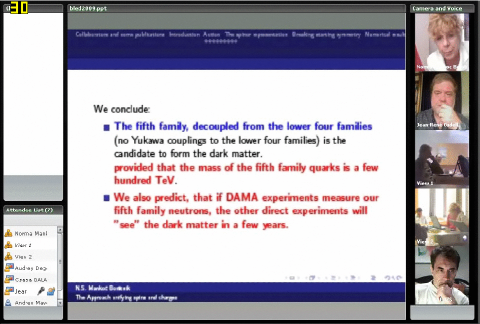
Figure 22: Bled Conference Discussion Bled-Moscow-CERN-Australia-Marburg-Liege

0.56 Conclusions

Staring to learn how one can use very efficiently the via conference facilities for discussing at least on very well defined questions the organizers and participants enjoyed very much this possibility. One can learn more about the possibilities of the video conferences in the explanation of M. Khlopov.

Discussion Section On the Witten’s No Go Theorem for the Kaluza-Klein-like Theories D. Lukman¹, N. S. Mankoč Borštnik¹ and H. B. Nielsen²

In this proceedings there is the talk of the same three authors, in which one step further towards realistic Kaluza-Klein-like theories is presented. The idea of Kaluza and Klein that the charges follow from the properties (dynamics) in higher dimensions is such a beautiful idea, that the authors can hardly accept the possibility that it has no application in nature. Particularly one of the authors, with her proposed ”approach unifying spin and charges”, offering also the mechanism for generating families, which is a kind of the Kaluza-Klein-like theory, is trying hard to find the way out of the ”no-go” theorem of Witten. The problem with Kaluza-Klein-like theories is that any break of symmetries seems to cause, if there are no special protections, that a massless fermion of one handedness gain after the break the mass of the scale of breaking.

The authors discuss in several papers hnkk06 ; hn07 and published talks possibilities that breaks of the symmetries might not always end up with massive fermions. The proposed loop hole through the Witten’s ”no-go theorem” was the appearance of the appropriate boundaries for a toy model with $(1+5)$-dimensional space.

In the work presented in this proceedings (and also in the previous one, except that a further step was made) the hope for cases when the manifold in all the higher dimensions, except two, is flat, and which the authors call ”an effective two dimensionality” cases is found. Namely, in the case of a spinor in $d=(1+(d-1))$ compactified on an (formally) infinite disc with the zweibein which makes a disc curved on $S^{2}$ and with the spin connection field which allows on such a sphere only one massless spinor state of a particular charge, the massless spinor does chirally couple to the corresponding Kaluza-Klein gauge field. In $d=2$, namely, the equations of motion following from the action with the linear curvature leave spin connection and zweibein undetermined

Discussions Section On the Fifth Family Proposed by the ”Approach Unifying Spin and Charges” and the Dark Matter Content G. Bregar and N.S. Mankoč Borštnik

0.57 What speaks for the conclusion that the fifth family members with the quark masses of a few hundred TeV/$c^{2}$ and the neutrino mass of a few TeV/$c^{2}$ are the candidates to form the dark matter, and what might speak against it? What speaks for the antibaryon $\bar{u}_{5}\bar{u}_{5}\bar{u}_{5}$ to be the stable particle?

0.57.1 A short review of the ”approach unifying spin and charges” from the point of view of the dark matter candidates.

Let us first point out those details of the ”approach unifying spin and charges”, which seem to be connected with possible answers to the question put in the title of this section 0.57:
What speaks for the conclusion that the fifth family members with the quark masses of a few hundred TeV/$c^{2}$ and the neutrino mass of a few TeV/$c^{2}$ are the candidates to form the dark matter?

The reader can find more about the ”approach” in the talk of Norma and the references therein, as well as in the other two talks, whose coauthor is Norma and in gn2pn06 .

First let us point out that the ”approach” is offering the mechanism for the appearance of families by introducing the second kind of the Clifford algebra objects, which generates families as the equivalent representations to the Dirac spinor representation. Accordingly the number of families is determined by the ”approach” and there is no freedom to make a choice of the number of families, let say, by the choice of an appropriate group, which would allow a chosen number of stable or unstable families. Let us say that this is not the case for other models where the number of families are put in by hand, at least by a choice of an appropriate group.

The ”approach” predicts from the simple starting action in the energy region bellow the unification scale of the three observed charges two times four families. The upper four families are decoupled in the Yukawa couplings from the lower four families.

Due to the ”approach” particular spontaneous break of the starting symmetries of the spinor and the gauge fields (vielbeins and the two kinds of the spin connection fields), leads to massive upper four families and massless lower four families. The lower four families have all the properties assumed by the ”standard model of the electroweak and colour interactions” before the electroweak break. The electroweak break influences the properties of the lower and upper four families. The quarks of the fourth of the lower four families are predicted (the references are in the talk of Norma) to have masses at around $250$ GeV/$c^{2}$ or above and the lepton masses are predicted to be at around $100$ GeV/$c^{2}$ or above. The fifth family, with no Yukawa couplings to the lower four families, is accordingly stable and therefore the candidate for forming the dark matter constituents.

The accurate prediction of the fifth family masses is at this stage of the development of the ”approach” not yet possible. Too many problems have to be solved first, like:
i. We must treat in a trustful way the nonperturbative breaking of a starting symmetry, explaining how does the break occur and why.
ii. We must derive the Yukawa couplings beyond the tree level and show that this calculations explain drastic differences in the properties of u-quark, d-quark, neutrino and electron.
iii. We must understand all the discrete symmetries following from the ”approach”.
iv. We must study possible phase transitions connected with the groups, which symmetries break.
v. And several others.

Following the evolution of the fifth family members in the expanding universe up to present dark matter density for different choices of the fifth family masses and evaluating the properties of the fifth family members when scattering on the ordinary (mainly formed of the first family members) matter can help to better understand the problems presented above and to easier find the way of solving them.

We start to follow the number density of our fifth family members when the temperature was high enough that the fifth family quarks and antiquarks, leptons and antileptons were in thermal equilibrium with the plasma to which all the massless gauge and scalar fields and all the massless families contribute. The expansion causes that the plasma cools down and makes less and less possible the generation of massive quarks and antiquarks out of the plasma. Massive fifth family members start to decouple since they have less and less occasion to meet their antiparticles. Scattering of the plasma constituents on clusters of the fifth family quarks destroys the clusters unless the temperature falls appreciably bellow the binding energy of the clusters. Then the clusters start to form and decouple out of plasma.

If the fifth family quark masses are of the order $100$ TeV/$c^{2}$, is the binding energy of the order of $1$ TeV/$c^{2}$ and our calculations show that the number density of the colourless fifth family neutrons is, when the temperature lowers to the colour phase transition temperature (to $1$ GeV/$k_{b}$), of the same order of magnitude as the number density of the fifth family quarks and antiquarks. The colour phase transition causes huge enlargement of the scattering cross sections of all the quarks and antiquarks and of coloured objects and dresses the quarks with $\approx 300$ MeV/$c^{2}$, while the colourless neutrons are too strongly bound to feel the phase transition at all. Due to huge enlargement of the scattering cross sections the fifth family quarks and antiquarks either annihilate or form colourless objects and deplete out of the rest of plasma long before the temperature of the plasma falls bellow $1$ MeV/$k_{b}$ when the first family quarks can start to form bound states either among themselves or with the fifth family members.

If the fifth family quark masses are of the order $300$ MeV/$c^{2}$, as Maxim is assuming, then their binding energy is of the order of a few MeV/$c^{2}$ and the number density of the colourless baryons is at the colour phase transition (T=$1$ GeV/$k_{b}$) negligible. The colour phase transition, enlarging very much the scattering cross section, causes annihilation of a large amount of the fifth family quarks and antiquarks, the formation of the colourless objects and, if the fifth family antibaryon-baryon asymmetry is assumed, as Maxim and his group does, also the colourless object (for a particular choice of the baryon-antibaryon asymmetry) of $\bar{u}_{5}\bar{u}_{5}\bar{u}_{5}$. Those that succeed to survive as an coloured object at $1$ MeV/$k_{b}$ start to form the colourless objects with the first family quarks. Maxim and his group claim that there are $\bar{u}_{5}\bar{u}_{5}\bar{u}_{5}$ that mostly survive forming with He nuclei the electric chargeless objects.

For masses of the fifth family quarks and antiquarks above few hundred TeV/$c^{2}$ the fifth family baryon-antibaryon asymmetry makes no difference, as long as the approximations we made when evaluating properties of the fifth family members in the evolution of the universe are meaningful.

For masses close to one TeV/$c^{2}$ or bellow the baryon-antibaryon asymmetry starts to be essential (as it is for the first family members).

In the next subsection we discuss the evaluations we made to estimate properties of the fifth family members by studying their behaviour in the evolution of the universe and when scattering on the ordinary matter. We shall point out those approximations, which need to be treated more accurately, although for most of these points more accurate treatment appears as a very demanding project.

Let us point out that we started to follow the behaviour of the fifth family members for the masses far above $1$ TeV/$c^{2}$ after all the breaks except the electroweak break took place.

0.57.2 The stable fifth family members in the expanding universe if the fifth family neutron and the fifth family neutrino is the lightest baryon and lepton, respectively.

If the mass of the stable fifth family neutrino is a few TeV/$c^{2}$ or above and of the stable fifth family neutron a few hundred TeV/$c^{2}$ or above, these neutrons and neutrinos are the candidates to be the constituents of the dark matter, fulfilling all the requirements for the dark matter, from either the cosmological observations or direct measurements of any kind. However, in the paper of Gregor and Norma gn2gn , we were not yet able to determine the relative contribution of these two components of the dark matter.

Let us point out the approximations we have done when treating the fifth family members as the candidates to form the dark matter:

• We assumed that in the interval region of temperatures from $\frac{m_{q_{5}}c^{2}}{k_{b}}$ to a GeV/$k_{b}$ (which is the temperature of the $SU(3)$ phase transition), in which we calculated the number density of the fifth family quarks and antiquarks, and the fifth family neutrons, the one gluon exchange is the dominant contribution to the interaction among quarks. This assumption is the meaningful one.

• We evaluated in the Bohr like model the binding energy and the potential among the fifth family baryons with the assumption that the fifth family quarks interact dominantly with the one gluon exchange. Also this assumption does not seem questionable.

• When solving the coupled Boltzmann equations for the number density of quarks and the number density of coloured and colourless clusters, we needed the scattering amplitudes, presented in Eq.(2) of the paper gn2gn . The expressions for the scattering cross sections of Eq.(2) are very approximate, and we corrected their accuracy with the parameters $\eta_{c_{5}}$, which takes into account that the clusters of two quarks bind into the clusters of three quarks, and $\eta_{(q\bar{q})_{b}}$, which takes into account the roughness of the estimation. These two cross sections should be calculated more precisely, so that we could limit the interval, within which both $\eta$’s lie. These calculations might influence considerably the conclusions.

• The colourless fifth family baryons, tied strongly into very small clusters, do not feel colour phase transition when it occurs at around $1$ GeV, while the coloured quarks and antiquarks or the coloured clusters of two quarks or antiquarks do. At the colour phase transition all the quarks of any family start to enlarge very much the scattering cross section. But while the fifth family quarks with masses of several hundred TeV/$c^{2}$ and accordingly of the binding energy into the corresponding clusters of several TeV start to bind at $1$ GeV, the first family quarks can not until the temperature falls below the binding energy of ”dressed” first family quarks, that is bellow a few MeV. We evaluated that the fifth family quarks and antiquarks either annihilate or form the colourless objects and deplete soon after $1$ GeV, so that there is a negligible amount available below a few MeV to form clusters with the first family members. It is a hard project to treat the colour phase transition, although we should do this.

• The references treating neutrinos with masses above few TeV as candidates for the dark matter constituents gn2dolgov ; gn2maxim report that the large scattering amplitudes for such neutrinos cause strong annihilation of neutrinos lowering accordingly their possible contribution to the dark matter. For the mass region of the neutrino from $10$ TeV/$c^{2}$ to $100$ TeV/$c^{2}$ the scattering amplitudes were only roughly estimated so far. The estimation in the mass interval of a few TeV/$c^{2}$ up to $100$TeV/$c^{2}$ seems accordingly not to contradict the measured dark matter density, which means that the fifth family neutrinos with masses in this region do not contribute more than our fifth family neutrons. In the case of the fifth family quark masses of a few $100$ TeV/$c^{2}$ and the fifth family neutrino mass of a few TeV/$c^{2}$ it seems reasonable to conclude that the dark matter consists either mostly of the fifth family neutrons, or of the fifth family neutrinos or of both. However, more in-depth studies are needed to make final conclusions.

• The evaluations of the interaction of the fifth family neutrons with the ordinary matter, although very approximate, brought the conclusion that the fifth family baryons are the acceptable dark matter constituents. Also these estimations are quite rough. Taking into account the uncertainties in knowing the local properties of the dark matter, we can conclude that the fifth family members are the right candidates to form the dark matter, provided that the neutron is the lightest baryon and the neutrino the lightest lepton.

Can it be that not the neutron but, let say, proton or some other fifth family baryon is the stable fifth family baryon? Would this change the conclusion that the fifth family is an acceptable candidate to form the dark matter? $n_{5}$ is the lightest baryon when the masses of $u_{5}$ and $d_{5}$ are in relative separation of the order of magnitude $10^{-4}$. The possibilities that $u_{5}u_{5}u_{5}$ or $d_{5}d_{5}d_{5}$ or $u_{5}u_{5}d_{5}$ are the lightest baryons are under considerations now.

Let us point out that our evaluations with the stable $n_{5}$ and $\nu_{5}$ predict that the CDMS or other experiments will measure the dark matter signals which will not contradict the DAMA results.

Can even very light fifth family members with masses of quarks of a few hundred MeV$/c^{2}$, as assumed by Maxim and his group, be a possible solution, if one assumes in addition a very particular fifth family antibaryon-baryon asymmetry? Maxim claims that it does. Norma has severe doubts that such assumptions can be fulfilled at all, not only within the ”approach unifying spins and charges” but within any model, which ”wants to be elegant”. But to say anything about the assumptions of the Maxim’s group in the context of the ”approach unifying spins and charges” one should study first the discrete symmetries, as well as the matter-antimatter asymmetry within this approach.

Discussions section On the Fifth Family Proposed by the ”Approach Unifying Spin and Charges” and the Dark Matter Content M.Yu. Khlopov

0.58 Composite dark matter with $\bar{u}_{5}\bar{u}_{5}\bar{u}_{5}$ constituent.

The ”approach unifying spin and charges” predicts that the lightest particles of fifth family are stable and are therefore the candidates for the dark matter. The ”approach” assumes that they are very heavy and can be hardly produced and studied at accelerators. One has to use analysis of cosmological evolution for different mass ratios and make a conclusion on the consistency of its results with observations.

In view of unknown mass ratio of the fifth family quarks the possibilities can be considered that charged $u_{5}u_{5}u_{5}$ or $d_{5}d_{5}d_{5}$ or $u_{5}u_{5}d_{5}$ are the lightest baryons. If they are treated as dark matter candidates in charge symmetric case, the results of the analysis mkd2Q leave practically no room for consistency of such possibilities with cosmology. The only possibility that does not meet immediate troubles is to use composite dark matter scenario with excessive $\bar{u}_{5}\bar{u}_{5}\bar{u}_{5}$ as its constituent.

0.58.1 Brief review of composite dark matter models

It was shown in mkd2I ; mkd2Q ; mkd2FKS ; mkd2KK that the existence of heavy stable -2 charged particles, being in excess over their antiparticles and forming atom-like neutral O-helium bound state with primordial helium, is compatible with all the experimental constraints. In this case composite dark matter scenario of nuclear interacting Warmer than Cold Dark Matter. Such scenario can be realized for a wide range of -2 charged particles masses, including 100 TeV range. For the masses of OHe $m_{o}\sim 1$TeV this new form of dark matter can provide explanation of excess of positron annihilation line radiation, observed by INTEGRAL in the galactic bulge. Such explanation mkd2KK is based on the calculation of the rate of E0 transitions in O-helium atoms, excited in collisions in the central part of Galaxy. The rate of such collisions decreases as $\propto m_{o}^{-2}$ and cannot explain INTEGRAL data for masses about 100 TeV. The search for stable -2 charge component of cosmic rays is challenging for PAMELA and AMS02 experiments. However such fraction decreases inversely proportional $m_{o}$ and can also be out reach of cosmic ray experiments for the mass around 100 TeV. Decays of heavy charged constituents of composite dark matter can provide explanation for anomalies in spectra of cosmic high energy positrons and electrons, observed by PAMELA, FERMI and ATIC. For the ”approach unifying spins and charges” this possibility needs special study, but seems hardly possible. In the context of the approach mkd2I ; mkd2Q ; mkd2FKS ; mkd2KK search for heavy stable charged quarks and leptons at LHC acquires the significance of experimental probe for components of cosmological composite dark matter. Such search is restricted by masses $m_{o}\leq 1$TeV and is impossible for 100 TeV quarks of fifth family.

The results of dark matter search in experiments DAMA/NaI and DAMA/ LIBRA can be explained in the framework of composite dark matter scenario without contradiction with negative results of other groups. This scenario can be realized in different frameworks, in particular, in the extensions of Standard Model, based on the approach of almost commutative geometry mkd2FKS , in the model of stable quarks of 4th generation mkd2I ; mkd2Q that can be naturally embedded in the heterotic superstring phenomenology, in the models of stable technileptons and/or techniquarks mkd2KK , following from Minimal Walking Technicolor model. It might be also possible in the approach unifying spin and charges.

The proposed explanation of the puzzles of direct dark matter searches is based on the mechanism of low energy binding of OHe with nuclei. The following picture is assumed: at the distances larger, than its size, OHe is neutral and it feels only Yukawa exponential tail of nuclear attraction, due to scalar-isoscalar nuclear potential. It should be noted that scalar-isoscalar nature of He nucleus excludes its nuclear interaction due to $\pi$ or $\rho$ meson exchange, so that the main role in its nuclear interaction outside the nucleus plays $\sigma$ meson exchange, on which nuclear physics data are not very definite. When the distance from the surface of nucleus becomes smaller than the size of OHe, the mutual attraction of nucleus and OHe is changed by dipole Coulomb repulsion. Inside the nucleus strong nuclear attraction takes place. In the result a specific spherically symmetric potential appears and the solution of Schrodinger equation with such potential for the OHe- nucleus suystem can be found. Within the uncertainty of nuclear physics parameters there exists a range at which OHe binding energy with sodium and/or iodine is in the interval 2-6 keV. Radiative capture of OHe to this bound state leads to the corresponding energy release observed as an ionization signal in DAMA detector.

OHe concentration in the matter of underground detectors is determined by the equilibrium between the incoming cosmic flux of OHe and diffusion towards the center of Earth. It is rapidly adjusted and follows the change in this flux with the relaxation time of few minutes. Therefore the rate of radiative capture of OHe should experience annual modulations reflected in annual modulations of the ionization signal from these reactions.

An inevitable consequence of the proposed explanation is appearance in the matter of DAMA/NaI or DAMA/LIBRA detector anomalous superheavy isotopes of sodium and/or iodine, having the mass roughly by $m_{o}$ larger, than ordinary isotopes of these elements. If the atoms of these anomalous isotopes are not completely ionized, their mobility is determined by atomic cross sections and becomes about 9 orders of magnitude smaller, than for O-helium. It provides their conservation in the matter of detector. Therefore mass-spectroscopic analysis of this matter can provide additional test for the O-helium nature of DAMA signal. Methods of such analysis should take into account the fragile nature of OHe-Na bound states, since their binding energy is only few keV.

With the account for high sensitivity of the numerical results to the values of nuclear parameters and for the approximations, made in the calculations, the presented results mkd2Bled09 can be considered only as an illustration of the possibility to explain puzzles of dark matter search in the framework of composite dark matter scenario. An interesting feature of this explanation is a conclusion that the ionization signal expected in detectors with the content, different from NaI, can be dominantly in the energy range beyond 2-6 keV. Therefore test of results of DAMA/NaI and DAMA/LIBRA experiments by other experimental groups can become a very nontrivial task. In particular, energy release in reaction of OHe binding with germanium in CDMS detector is beyond the range 2-6 keV and this conclusion becomes stronger with the growth of $m_{o}$ as show the results of our calculations presented in these Proceedings. This feature corresponds to the recent analysis of CDMS data mkd2Kamaev:2009gp , claiming that ionization energy release in the range of DAMA signal (2-6 keV) is excluded with the significance of 6 standard deviations.

To prove to be an explanation for DAMA results, the composite dark matter scenario should reproduce the detected signal. A straightforward calculation of the rate of radiative capture of nuclei by OHe is now under way. The number of events is determined by the product of this rate and the equilibrium concentration of OHe in detector, which in turn is adjusted to the incoming flux. The latter is inversely proportional to the mass of OHe. Therefore the results of this calculations will provide information on the preferable mass of OHe, determined by its -2 charged constituent.

0.58.2 Can composite dark matter scenario take place in the approach, unifying spins and charges?

In the case of approach, unifying spins and charges, composite dark matter scenario mkd2I ; mkd2Q ; mkd2FKS ; mkd2KK can be realized completely for masses of $u_{5}$ about few hundred GeV. This realization assumes the necessary excess of $\bar{u}_{5}$ and can provide explanation for DAMA/CDMS controversy and positron excess observed by INTEGRAL. Decays of $\bar{u}_{5}$ can explain excess of high energy electrons observed by FERMI and ATIC, but in the absence of subdominant +2 charged component positron anomalies can not be explained. This scenario with low mass quarks is, however, very implausible in the framework of ”approach”, since the masses of the stable family are assumed to be very close to the third family masses.

For the case of 100 TeV mass quarks, the possibility to explain INTEGRAL data and high energy cosmic electron anomaly is lost. However, these phenomena can find explanation with the use of natural astrophysical sources and may not imply effects of dark matter. Then only DAMA/CDMS controversy should be explained, and such explanation is shown to be possible mkd2Bled09 .

Let us stipulate some necessary steps in further development of this scenario:

• The mechanism of baryosynthesis should be developed in the ”approach”. This mechanism can be directly applied also to the fifth family. If not, and only first family baryon asymmetry is initially formed, sphaleron transitions would redistribute the excess of particles and create the excess of fifth quarks. For composite dark matter scenario the excess of antiquarks is needed and the conditions under which the asymmetry in baryons of fifth family has opposite sign relative to the first family baryon asymmetry should be studied.

• Self-consistent analysis should also clarify the role of fifth neutrino in this scenario.

• If OHe hypothesis is correct, it should give the amount of events in NaI, corresponding to the detected signal. It implies quantum- mechanical calculation of the rate of OHe-nucleus radiative capture.

• The calculated rate of OHe-nucleus radiative capture should be used for reproduction of DAMA signal with account for all the physical and astrophysical uncertainties.

0.59 Some conclusions for future work

It is mutually agreed that stability of the fifth family is very well motivated in the approach, unifying spins and charges. It gives rise to various possible candidates for stable lightest particles (heavy quark clusters) and correspondingly different dark matter scenarios. Tests of these scenarios along the lines of the present discussion are challenging for our future joint work.

Discussions Section On the Yukawa Couplings Proposed by the ”Approach Unifying Spin and Charges” Beyond the Tree Level A. Hernández-Galeana¹ and N.S. Mankoč Borštnik²

0.60 A short introduction I, written by Norma

The ”approach unifying spin and charges”, proposed by Norma Susana Mankoč Borštnik, predicts two kinds of the Yukawa couplings. One kind distinguishes on the tree level only among the members of one family (among the u-quark, d-quark, neutrino and electron), while the other kind distinguishes only among the families. Beyond the tree level both kinds of the Yukawa couplings start to contribute coherently and a detailed study should manifest the drastic differences in properties of quarks and leptons: in their masses and mixing matrices. The reader can find the explanation for this statement in the contribution presented in this proceedings on page 119 by Norma and in the references therein). This is a very demanding project. To understand how does this occur we start this study first on a toy model. This work is the introduction into first steps towards understanding the properties of the lower four families of quarks and leptons as predicted by the ”approach”, by using a toy model. Albino has made first step which could help to do calculations beyond the tree level for the ”approach unifying spin and charges”.

0.61 The introduction II and all the rest, written by Albino

We make the first step which could help to do calculations beyond the tree level for the ”approach unifying spin and charges”. We propose a tentative hierarchical mass generation mechanism for one sector; u, d, e or $\nu$, where the mass of the heaviest ordinary family is generated from a See-saw mechanism, meanwhile light fermions obtain masses from radiative corrections, at one and two loops, respectively. These radiative corrections could be mediated either by scalar or gauge boson fields within the ”approach unifying spin and charges”.

0.62 Tree level mass matrix

For a given sector; u (up quarks), d (down quarks), e (charged leptons) or $\nu$ (neutrinos), $f_{1}\;,f_{2}\;,f_{3}$ denote ordinary families, and F corresponds to the fourth very heavy family. Let us start by assuming the tree level mass terms

$$m_{34}\>\bar{f_{3L}^{o}}\>F_{R}^{o}+m_{43}\>\bar{F_{L}^{o}}\>f_{3R}^{o}+M\>\bar{F_{L}^{o}}\>F_{R}^{o}+h.c.=\bar{\psi_{L}^{o}}\>{\cal M}_{o}\>\psi_{R}^{o}+h.c.$$ (343)

where

$$\psi_{oL}^{T}=(f_{1}^{o},f_{2}^{o},f_{3}^{o},F^{o})_{L}\qquad,\qquad\psi_{oR}^{T}=(f_{1}^{o},f_{2}^{o},f_{3}^{o},F^{o})_{R}$$ (344)

are weak or interaction eigenfields. For the sake of simplicity, let us assume that it is possible to set $m_{34}=m_{43}\equiv p$, such that, we may write ${\cal M}_{o}$ in Eq. (1) as the real and symmetric ”See-saw” type mass matrix

$${\cal M}_{o}=\begin{pmatrix}0&0&0&0\\ 0&0&0&0\\ 0&0&0&p\\ 0&0&p&M\end{pmatrix}\;;\qquad M>p>0\>.$$ (345)

Using an orthogonal matrix $V^{o}$ to diagonalize ${\cal M}_{o}$; $\Psi^{o}_{L}=V^{o}\>\chi_{L}^{o}\;,\;\Psi^{o}_{R}=V^{o}\>\chi_{R}^{o}\;,$

$$\bar{\psi_{L}^{o}}\>{\cal M}_{o}\>\psi_{R}^{o}=\bar{\chi_{L}^{o}}\>{V^{o}}^{T}\>{\cal M}_{o}\>V^{o}\>\chi_{R}^{o}\>,$$ (346)

where $T$ means transpose, and we write $V^{o}$ as

$$V^{o}=\left(\begin{array}[]{ccrr}1&0&0&0\\ 0&1&0&0\\ 0&0&\cos{\alpha}&\sin{\alpha}\\ 0&0&-\sin{\alpha}&\cos{\alpha}\end{array}\right)\>,$$ (347)

where the two nonzero eigenvalues $\lambda_{3}$ and $\lambda_{4}$ of ${\cal M}_{o}$ satisfy

$$\lambda^{2}-M\lambda-p^{2}=0,\quad M=\lambda_{3}+\lambda_{4},\quad-p^{2}=\lambda_{3}\>\lambda_{4}$$ (348)

$$\lambda_{3}=\frac{1}{2}\left(M-\sqrt{M^{2}+4p^{2}}\right)<0\qquad,\qquad\lambda_{4}=\frac{1}{2}\left(M+\sqrt{M^{2}+4p^{2}}\right)>0$$ (349)

$$\cos{\alpha}=\sqrt{\frac{\lambda_{4}}{\lambda_{4}-\lambda_{3}}}\quad,\quad\sin{\alpha}=\sqrt{\frac{-\lambda_{3}}{\lambda_{4}-\lambda_{3}}}\quad,\quad\cos{\alpha}\sin{\alpha}=\frac{p}{\lambda_{4}-\lambda_{3}}$$ (350)

$$-\lambda_{3}\>\cos^{2}{\alpha}=\lambda_{4}\>\sin^{2}{\alpha}=\frac{p^{2}}{\lambda_{4}-\lambda_{3}}\equiv m_{o}$$ (351)

$${V^{o}}^{T}\>{\cal M}_{o}\>V^{o}=Diag(0,0,\lambda_{3},\lambda_{4})$$ (352)

Eqs. (347-352) are exact analytic results from the diagonalization of ${\cal M}_{o}$.

Note that if we impose the hierarchy $\frac{|\lambda_{3}|}{\lambda_{4}}\ll 1$, then

$$\frac{p^{2}}{M^{2}}=\frac{|-p^{2}|}{M^{2}}=\frac{|\lambda_{3}\lambda_{4}|}{(\lambda_{3}+\lambda_{4})^{2}}=\frac{|\lambda_{3}|}{\lambda_{4}}\frac{1}{(1+\frac{\lambda_{3}}{\lambda_{4}})^{2}}\ll 1\;.$$ (353)

In this limit, we may approach

$$\lambda_{3}\thickapprox-\frac{p^{2}}{M}\qquad,\qquad\lambda_{4}\thickapprox M+\frac{p^{2}}{M}\thickapprox M\;,$$

$$\sin{\alpha}=\sqrt{\frac{-\lambda_{3}}{\lambda_{4}-\lambda_{3}}}\approx\sqrt{\frac{p^{2}}{M^{2}}}=\frac{p}{M}\ll 1\;,$$ (354)

$$\cos{\alpha}\sin{\alpha}=\frac{p}{\lambda_{4}-\lambda_{3}}\approx\frac{p}{M}\ll 1\;,$$

in agreement with the well known results from See-saw mass matrix. $-\lambda_{3}$ may be associated, in good approximation, with the mass for the heaviest ordinary fermion $m_{t}$, $m_{b}$, $m_{\tau}$ or $m_{3}$, and $\lambda_{4}$ with the mass of the heavy fourth fermion in a given sector.

0.63 One loop corrections

Subsequently, the masses for the light fermions would arise through one and two loops radiative corrections, respectively. To achieve this goal, let us introduce the gauge bosons $Y_{1}\;,Y_{3}\;,Z_{1}\;,Z_{3}$, with the gauge couplings to fermions in the interaction basis as

$$\left(h_{12}\>\bar{f_{1L}^{o}}\gamma_{\mu}\>f_{2L}^{o}+h_{23}\>\bar{f_{2L}^{o}}\gamma_{\mu}\>f_{3L}^{o}\right)Y_{1}^{\mu}+h_{33}\>\bar{f_{3L}^{o}}\gamma_{\mu}\>f_{3L}^{o}\>Y_{3}^{\mu}\\ \\ +\left(H_{12}\>\bar{f_{1R}^{o}}\gamma_{\mu}\>f_{2R}^{o}+H_{23}\>\bar{f_{2R}^{o}}\gamma_{\mu}\>f_{3R}^{o}\right)Z_{1}^{\mu}+H_{33}\>\bar{f_{3R}^{o}}\gamma_{\mu}\>f_{3R}^{o}\>Z_{3}^{\mu}+h.c.$$ (355)

where $h_{12}$, $h_{23}$, $h_{33}$, $H_{12}$, $H_{23}$, and $H_{33}$ are gauge coupling constants. We also assume the gauge boson mass matrix:

$$X^{T}\>M_{B}^{2}\>X\qquad,\qquad X^{T}=(Y_{1},Y_{3},Z_{3},Z_{1})\;,$$ (356)

with

$$M_{B}^{2}=\left(\begin{array}[]{cccc}a_{1}&b&0&0\\ b&a_{2}&c&0\\ 0&c&a_{3}&d\\ 0&0&d&a_{4}\end{array}\right).$$ (357)

These mass terms for gauge(or scalar) fields in Eq.(357) should be generated at some stage of symmetry breaking at the scale $\Lambda\>>(\mbox{or may be}\>\gg$) than the electroweak scale $v\approx 246\>GeV$. The diagonalization of $M_{B}^{2}$ is performed in the Appendix B. Using the gauge boson couplings, Eq.(355), and the tree level mass terms (See-saw mechanism), Eq.(343), we can construct the one loop mass diagrams of Fig. 23.

Figure 23: One loop contributions to: a) $m_{22}^{(1)}\>\bar{f_{2L}^{o}}\>f_{2R}^{o}$, b) $m_{23}^{(1)}\>\bar{f_{2L}^{o}}\>f_{3R}^{o}$, c) $m_{32}^{(1)}\>\bar{f_{3L}^{o}}\>f_{2R}^{o}$, d) $m_{33}^{(1)}\>\bar{f_{3L}^{o}}\>f_{3R}^{o}$

The evaluation of these diagrams yields the one loop mass terms contributions

$$m_{22}^{(1)}\>\bar{f_{2L}^{o}}\>f_{2R}^{o}+m_{23}^{(1)}\>\bar{f_{2L}^{o}}\>f_{3R}^{o}+m_{32}^{(1)}\>\bar{f_{3L}^{o}}\>f_{2R}^{o}+m_{33}^{(1)}\>\bar{f_{3L}^{o}}\>f_{3R}^{o}\;,$$ (358)

with

$$m_{22}^{(1)}=\frac{h_{23}H_{23}}{16\pi^{2}}\sum_{k=1,2,3,4;\,i=3,4}m_{i}^{(o)}\>(V^{o})_{3i}^{2}\>U_{1k}U_{4k}\>f(M_{k},m_{i}^{(o)}),$$ (359)

$$m_{23}^{(1)}=\frac{h_{23}H_{33}}{16\pi^{2}}\sum_{k=1,2,3,4;\,i=3,4}m_{i}^{(o)}\>(V^{o})_{3i}^{2}\>U_{1k}U_{3k}\>f(M_{k},m_{i}^{(o)}),$$ (360)

$$m_{32}^{(1)}=\frac{h_{33}H_{23}}{16\pi^{2}}\sum_{k=1,2,3,4;\,i=3,4}m_{i}^{(o)}\>(V^{o})_{3i}^{2}\>U_{2k}U_{4k}\>f(M_{k},m_{i}^{(o)}),$$ (361)

$$m_{33}^{(1)}=\frac{h_{33}H_{33}}{16\pi^{2}}\sum_{k=1,2,3,4;\,i=3,4}m_{i}^{(o)}\>(V^{o})_{3i}^{2}\>U_{2k}U_{3k}\>f(M_{k},m_{i}^{(o)}),$$ (362)

where $m_{3}^{(o)}=\lambda_{3}$, $m_{4}^{(o)}=\lambda_{4}$, Eqs.(349,353), $U$ is the orthogonal matrix which diagonalizes $M_{B}^{2}$,Eqs.(422,429), with

$$B_{i}=U_{ij}\omega_{j}\quad,\quad B_{1}=Y_{1}\quad,\quad B_{2}=Y_{3}\quad,\quad B_{3}=Z_{3}\quad,\quad B_{4}=Z_{1}$$ (363)

being the relation between interaction and mass boson eigenfields $\omega_{i}$, $i,j=1,2,3,4$, $M_{k}^{2}$ are the eigenvalues of $M_{B}^{2}$, and

$$f(a,b)\equiv\frac{a^{2}}{a^{2}-b^{2}}\ln{\frac{a^{2}}{b^{2}}}\;.$$ (364)

Performing the summation over the index $i=3,4$ in Eqs.(359-362), and using the relations in Eqs.(350,351), we may write

$$m_{22}^{(1)}=\frac{h_{23}H_{23}}{16\pi^{2}}m_{o}\sum_{k}U_{1k}U_{4k}F(M_{k})\quad,\quad m_{23}^{(1)}=\frac{h_{23}H_{33}}{16\pi^{2}}m_{o}\sum_{k}U_{1k}U_{3k}F(M_{k})\>,$$ (365)

$$m_{32}^{(1)}=\frac{h_{33}H_{23}}{16\pi^{2}}m_{o}\sum_{k}U_{2k}U_{4k}F(M_{k})\quad,\quad m_{33}^{(1)}=\frac{h_{33}H_{33}}{16\pi^{2}}m_{o}\sum_{k}U_{2k}U_{3k}F(M_{k})\>,$$ (366)

where the mass parameter $m_{o}$ is defined in Eq.(351), and

$$F(M_{k})\equiv\frac{M_{k}^{2}}{M_{k}^{2}-\lambda_{4}^{2}}\ln{\frac{M_{k}^{2}}{\lambda_{4}^{2}}}-\frac{M_{k}^{2}}{M_{k}^{2}-\lambda_{3}^{2}}\ln{\frac{M_{k}^{2}}{\lambda_{3}^{2}}}\>.$$ (367)

So, the one loop contribution in the interaction basis reads

$$\bar{\psi_{L}^{o}}\>{\cal M}_{1}^{o}\>\psi_{R}^{o}=\bar{\chi_{L}^{o}}\>{V^{o}}^{T}\>{\cal M}_{1}^{o}\>V^{o}\>\chi_{R}^{o}\qquad,\qquad{\cal M}_{1}^{o}=\left(\begin{array}[]{ccrr}0&0&0&0\\ 0&m_{22}^{(1)}&m_{23}^{(1)}&0\\ 0&m_{32}^{(1)}&m_{33}^{(1)}&0\\ 0&0&0&0\end{array}\right)\>,$$ (368)

and thus, up to one loop corrections, we get the mass terms

$$\bar{\chi_{L}^{o}}\left[{V^{o}}^{T}\>{\cal M}_{1}^{o}\>V^{o}+Diag(0,0,\lambda_{3},\lambda_{4})\right]\>\chi_{R}^{o}\equiv\bar{\chi_{L}^{o}}\>{\cal M}_{1}\>\chi_{R}^{o}\>,$$ (369)

with

$${\cal{M}}_{1}=\left(\begin{array}[]{clll}0&0&0&0\\ 0&m_{22}^{(1)}&m_{23}^{(1)}\cos\alpha&m_{23}^{(1)}\sin\alpha\\ 0&m_{32}^{(1)}\cos\alpha&\lambda_{3}+m_{33}^{(1)}\cos^{2}\alpha&m_{33}^{(1)}\cos\alpha\sin\alpha\\ 0&m_{32}^{(1)}\sin\alpha&m_{33}^{(1)}\cos\alpha\sin\alpha&\lambda_{4}+m_{33}^{(1)}\sin^{2}\alpha\end{array}\right)\>.$$ (370)

Remember now from Eq.(354) the value $\sin\alpha\ll 1$. In consistency with this tiny mixing angle, we assume that mixing between ordinary fermions with the fourth family, in each sector, is defined to leading order at the tree level by the see-saw mass matrix ${\cal M}_{o}$ in Eq.(345), and so, in this approach, we may neglect one loop corrections in what concern the mass and mixing of the fourth family with the ordinary ones, and then we may set $\sin\alpha=0$ in the mass matrix ${\cal M}_{1}$. Hence, we may approximate

$${\cal{M}}_{1}\approx\left(\begin{array}[]{clll}0&0&0&0\\ 0&m_{22}^{(1)}&m_{23}^{(1)}&0\\ 0&m_{32}^{(1)}&\lambda_{3}+m_{33}^{(1)}&0\\ 0&0&0&\lambda_{4}\end{array}\right)\>.$$ (371)

Thus, the diagonalization of ${\cal M}_{1}$ in this approach reduces to the diagonalization of a $2\times 2$ mass matrix as is done in the Appendix A. In terms of a biunitary transformation $\chi_{L}^{o}=V_{L}^{(1)}\;\chi_{L}^{1}$ and $\chi_{R}^{o}=V_{R}^{(1)}\;\chi_{R}^{1}$,

$$\bar{\chi_{L}^{o}}\>{\cal{M}}_{1}\>\chi_{R}^{o}=\bar{\chi_{L}^{1}}\;{V_{L}^{(1)}}^{T}{\cal{M}}_{1}\>V_{R}^{(1)}\;\chi_{R}^{1}\>.$$ (372)

With $c_{L,R}=\cos\theta_{L,R}$, $s_{L,R}=\sin\theta_{L,R}$ we may write

$$V_{L}^{(1)}=\left(\begin{array}[]{ccrc}1&0&0&0\\ 0&c_{L}&s_{L}&0\\ 0&-s_{L}&c_{L}&0\\ 0&0&0&1\end{array}\right)\quad\text{and}\quad V_{R}^{(1)}=\left(\begin{array}[]{ccrc}1&0&0&0\\ 0&c_{R}&s_{R}&0\\ 0&-s_{R}&c_{R}&0\\ 0&0&0&1\end{array}\right)\;,$$ (373)

where mixing angles $\sin\theta_{L}$ and $\sin\theta_{R}$ are defined in the Appendix A in terms of the eigenvalues $\sigma_{2}$ and $\sigma_{3}$, Eq.(407), and the parameters of ${\cal M}_{1}\>{\cal{M}}_{1}^{T}$ and ${{\cal M}_{1}}^{T}{\cal{M}}_{1}$, respectively. From $V^{(1)}_{L}$ and $V^{(1)}_{R}$ one computes

$${V^{(1)}_{L}}^{T}{\cal{M}}_{1}\>V^{(1)}_{R}=Diag(0,\sqrt{\sigma_{2}},-\sqrt{\sigma_{3}},\sqrt{\lambda_{+}})$$ (374)

$${V^{(1)}_{L}}^{T}{\cal{M}}_{1}\>{\cal{M}}_{1}^{T}\;V^{(1)}_{L}={V^{(1)}_{R}}^{T}{\cal{M}}_{1}^{T}\>{\cal{M}}_{1}\;V^{(1)}_{R}=Diag(0,\sigma_{2},\sigma_{3},\lambda_{+})\>.$$ (375)

Here $-\sqrt{\sigma_{3}}$ is a tiny correction to $\lambda_{3}$ in Eqs.(349,354).

0.63.1 Two loop contributions

We see from Eqs.(374,375) that up to one loop corrections the first family of ordinary fermions, $m_{u}$, $m_{d}$, $m_{e}$ or $m_{\nu 1}$ remain massless, and so we need to consider two loop contributions. We consider the two loop diagrams given in the Fig. 24.

Figure 24: Two loops contributions.

Let us recall that the transformations from massless (interaction) to mass eigenfields up to one loop are given by $\Psi^{o}_{L}=V^{o}\>\chi_{L}^{o}=V^{o}\>V^{(1)}_{L}\>\chi_{L}^{1}$ and $\Psi^{o}_{R}=V^{o}\>\chi_{R}^{o}=V^{o}\>V^{(1)}_{R}\>\chi_{R}^{1}$, where, explicitly

$$V^{o}\>V_{L}^{(1)} =\left(\begin{array}[]{crrc}1&0&0&0\\ 0&c_{L}&s_{L}&0\\ 0&-\cos\alpha\>s_{L}&\cos\alpha\>c_{L}&\sin\alpha\\ 0&\sin\alpha\>s_{L}&-\sin\alpha\>c_{L}&\cos\alpha\end{array}\right)\;,\;$$ (380)

$$V^{o}\>V_{R}^{(1)} =\left(\begin{array}[]{crrc}1&0&0&0\\ 0&c_{R}&s_{R}&0\\ 0&-\cos\alpha\>s_{R}&\cos\alpha\>c_{R}&\sin\alpha\\ 0&\sin\alpha\>s_{R}&-\sin\alpha\>c_{R}&\cos\alpha\end{array}\right)\>.$$ (385)

Using these field transformations to write the internal fermion lines in Fig. 24 in terms of the one loop mass eigenfieds, and performing a similar analysis as before, the two loop diagrams yields the contributions

$$m_{11}^{(2)}=\frac{h_{12}H_{12}}{16\pi^{2}}\sum_{k=1,2,3,4;\;i=2,3}m_{i}^{(1)}\>(V^{o}\>V_{L}^{(1)})_{2i}\>(V^{o}\>V_{R}^{(1)})_{2i}\>U_{1k}U_{4k}\>f(M_{k},m_{i}^{(1)}),$$ (386)

$$m_{21}^{(2)}=\frac{h_{23}H_{12}}{16\pi^{2}}\sum_{k=1,2,3,4;\;i=2,3}m_{i}^{(1)}\>(V^{o}\>V_{L}^{(1)})_{3i}\>(V^{o}\>V_{R}^{(1)})_{2i}\>U_{1k}U_{4k}\>f(M_{k},m_{i}^{(1)}),$$ (387)

$$m_{12}^{(2)}=\frac{h_{12}H_{23}}{16\pi^{2}}\sum_{k=1,2,3,4;\;i=2,3}m_{i}^{(1)}\>(V^{o}\>V_{L}^{(1)})_{2i}\>(V^{o}\>V_{R}^{(1)})_{3i}\>U_{1k}U_{4k}\>f(M_{k},m_{i}^{(1)}),$$ (388)

$$m_{31}^{(2)}=\frac{h_{23}H_{12}}{16\pi^{2}}\sum_{k=1,2,3,4;\;i=2,3}m_{i}^{(1)}\>(V^{o}\>V_{L}^{(1)})_{2i}\>(V^{o}\>V_{R}^{(1)})_{2i}\>U_{1k}U_{4k}\>f(M_{k},m_{i}^{(1)})\\ +\frac{h_{33}H_{12}}{16\pi^{2}}\sum_{k=1,2,3,4;\;i=2,3}m_{i}^{(1)}\>(V^{o}\>V_{L}^{(1)})_{3i}\>(V^{o}\>V_{R}^{(1)})_{2i}\>U_{2k}U_{4k}\>f(M_{k},m_{i}^{(1)}),$$ (389)

$$m_{13}^{(2)}=\frac{h_{12}H_{23}}{16\pi^{2}}\sum_{k=1,2,3,4;\;i=2,3}m_{i}^{(1)}\>(V^{o}\>V_{L}^{(1)})_{2i}\>(V^{o}\>V_{R}^{(1)})_{2i}\>U_{1k}U_{4k}\>f(M_{k},m_{i}^{(1)})\\ +\frac{h_{12}H_{33}}{16\pi^{2}}\sum_{k=1,2,3,4;\;i=2,3}m_{i}^{(1)}\>(V^{o}\>V_{L}^{(1)})_{2i}\>(V^{o}:V_{R}^{(1)})_{3i}\>U_{1k}U_{3k}\>f(M_{k},m_{i}^{(1)})\>.$$ (390)

Note that in the limit $M_{k}\gg m_{i}^{(1)}\;,i=2,3$, the function $f(a,b)$ behaves as $\ln{\frac{a^{2}}{b^{2}}}$. In this limit, using the one loop mass eigenvalues, $m_{2}^{(1)}=\sqrt{\sigma_{2}}$, $m_{3}^{(1)}=-\sqrt{\sigma_{3}}$, Eqs.(374,375), $V^{o}\>V_{L}^{(1)}$ and $V^{o}\>V_{R}^{(1)}$,Eq.(385), the relationships in Eqs.(414,415) and using the orthogonality of $U$, one gets

$$m_{11}^{(2)}=\frac{h_{12}H_{12}}{16\pi^{2}}m_{22}^{(1)}\>G_{14},$$ (391)

$$m_{21}^{(2)}=\frac{h_{23}H_{12}}{16\pi^{2}}\cos\alpha\>m_{32}^{(1)}\>G_{14},$$ (392)

$$m_{12}^{(2)}=\frac{h_{12}H_{23}}{16\pi^{2}}\cos\alpha\>m_{23}^{(1)}\>G_{14},$$ (393)

$$m_{31}^{(2)}=\frac{h_{23}H_{12}}{16\pi^{2}}\>m_{22}^{(1)}\>G_{14}+\frac{h_{33}H_{12}}{16\pi^{2}}\cos\alpha\>m_{32}^{(1)}\>G_{24},$$ (394)

$$m_{13}^{(2)}=\frac{h_{12}H_{23}}{16\pi^{2}}\>m_{22}^{(1)}\>G_{14}+\frac{h_{12}H_{33}}{16\pi^{2}}\cos\alpha\>m_{23}^{(1)}\>G_{13}$$ (395)

where the parameters $G_{14}$, $G_{24}$ and $G_{13}$ are defined as

$$G_{14} \equiv\sum_{k}U_{1k}U_{4k}\ln{\frac{M_{k}^{2}}{m_{o}^{2}}}\quad,\quad$$

$$G_{24} \equiv\sum_{k}U_{2k}U_{4k}\ln{\frac{M_{k}^{2}}{m_{o}^{2}}}\quad,\quad$$ (396)

$$G_{13} \equiv\sum_{k}U_{1k}U_{3k}\ln{\frac{M_{k}^{2}}{m_{o}^{2}}}$$

Hence, the leading order two loop contributions in the weak basis is written as $\bar{\psi_{L}^{o}}\>{\cal M}_{2}^{o}\>\psi_{R}^{o}$,

$${\cal M}_{2}^{o}\approx\left(\begin{array}[]{clll}m_{11}^{(2)}&m_{12}^{(2)}&m_{13}^{(2)}&0\\ m_{21}^{(2)}&0&0&0\\ m_{31}^{(2)}&0&0&0\\ 0&0&0&0\end{array}\right)\>.$$ (397)

So, up to two loops we obtain the mass terms

$$\bar{\chi_{L}^{1}}[\>(V_{o}V_{L}^{(1)})^{T}\>{\cal M}_{2}^{o}\>V_{o}V_{R}^{(1)}+Diag(0,\sqrt{\sigma_{2}},-\sqrt{\sigma_{3}},\lambda_{4})\>]\;\chi_{R}^{1}\equiv\bar{\chi_{L}^{1}}{\cal M}_{2}\;\chi_{R}^{1}\>,$$ (398)

where ${\cal{M}}_{2}\thickapprox$

$$\left(\begin{smallmatrix}m_{11}^{(2)}&m_{12}^{(2)}\>c_{R}-m_{13}^{(2)}\>\cos\alpha\>s_{R}&m_{13}^{(2)}\>\cos\alpha\>c_{R}+m_{12}^{(2)}\>s_{R}&\sin\alpha\>m_{13}^{(2)}\\ m_{21}^{(2)}\>c_{L}-m_{31}^{(2)}\>\cos\alpha\>s_{L}&\sqrt{\sigma_{2}}&0&0\\ m_{31}^{(2)}\>\cos\alpha\>c_{L}+m_{21}^{(2)}\>s_{L}&0&-\sqrt{\sigma_{3}}&0\\ \sin\alpha\>m_{31}^{(2)}&0&0&\lambda_{4}\end{smallmatrix}\right).$$ (399)

The diagonalization of ${\cal M}_{2}$ yields the physical masses for fermions in each sector u, d, e or $\nu$. Using the same arguments as before, we can perform this diagonalization in good approximation in the limit $\sin\alpha=0$. In this approach, the diagonalization of ${\cal{M}}_{2}$ reduces to diagonalize a $3\times 3$ mass matrix, and the results and/or method of diagonalization introduced in Ref.ah1u1 may be applied. Defining a new biunitary transformation $\chi_{L}^{1}=V_{L}^{(2)}\psi_{L}\;\mbox{and}\;\chi_{R}^{1}=V_{R}^{(2)}\psi_{R}$, then

$$\bar{\chi_{L}^{1}}\;{\cal{M}}_{2}\;\chi_{R}^{1}=\bar{\psi_{L}}\>{V_{L}^{(2)}}^{T}{\cal{M}}_{2}\>V_{R}^{(2)}\>\psi_{R}$$ (400)

where now

$${\Psi_{L}}^{T}=(f_{1L},f_{2L},f_{3L},F_{L})\quad,\quad{\Psi_{R}}^{T}=(f_{1R},f_{2R},f_{3R},F_{R})$$ (401)

are the mass eigenfields, that is

$${V_{L}^{(2)}}^{T}{\cal M}_{2}\;V_{R}^{(2)}=Diag(m_{1},m_{2},-m_{3},M_{F})\;.$$ (402)

$${V^{(2)}_{L}}^{T}{\cal{M}}_{2}\>{\cal M}_{2}^{T}\;V^{(2)}_{L}={V^{(2)}_{R}}^{T}{\cal M}_{2}^{T}\>{\cal{M}}_{2}\;V^{(2)}_{R}=Diag(m_{1}^{2},m_{2}^{2},m_{3}^{2},M_{F}^{2})\>.$$ (403)

For example: $m_{1}=m_{e}\;,\;m_{2}=m_{\mu}\;,\;m_{3}=-m_{\tau}\;,\;M_{F}=M_{E}\;$ for charged leptons.

Thus, the final transformations from massless (interaction) to mass fermion eigenfields are

$$\Psi_{L}^{o}=V^{o}\>V^{(1)}_{L}\>V^{(2)}_{L}\>\Psi_{L}\quad\mbox{and}\quad\Psi_{R}^{o}=V^{o}\>V^{(1)}_{R}\>V^{(2)}_{R}\>\Psi_{R}$$ (404)

0.64 Discussion

The basic assumptions in this Toy Radiative Corrections are: the tree level mass terms assumed in Eq.(343), the introduction of the gauge bosons fields $Y_{1}$, $Y_{3}$, $Z_{1}$, $Z_{3}$ and their couplings to fermions introduced in Eq.(355), as well as the structure of their mass matrix assumed in Eqs.(356,357). I have already taken a look to the “approach unifying spin and charges”; Proceedings, Portoroz, Slovenia 2003 and arXiv:0708.2846.

From this reading, it is not clear yet to me whether it is possible or not to accomplish (or give some arguments to justify) these basic assumptions for at least one of the sectors; u, d, e or $\nu$. In order to go further in this task, I would like to understand more details about the implementation of symmetry breaking within your approach. In any case, we can take this manuscript as one ”Toy specific example” which points out the way radiative corrections could arise, and the role they can play to implement a hierarchical spectrum of fermion masses.

0.65 Appendix A:
Diagonalization of a 2x2 mass matrix

Let us consider the diagonalization of the mass matrix

$$m=\left(\begin{array}[]{cc}m_{22}^{(1)}&m_{23}^{(1)}\\ m_{32}^{(1)}&\lambda_{3}+m_{33}^{(1)}\end{array}\right)\equiv\left(\begin{array}[]{cc}q_{2}&q_{23}\\ q_{32}&q_{3}\end{array}\right)\;.$$ (405)

We assume the signs: $q_{2}>0$, $q_{23}<0$, $q_{32}<0$, $q_{3}=\lambda_{3}+m_{33}^{(1)}\approx-\frac{p^{2}}{M}+m_{33}^{(1)}<0$

$$a_{L} =q_{2}^{2}+q_{23}^{2}, b_{L} =q_{3}^{2}+q_{32}^{2}, c_{L} =q_{2}q_{32}+q_{3}q_{23}$$ (406)

$$a_{R} =q_{2}^{2}+q_{32}^{2}, b_{R} =q_{3}^{2}+q_{23}^{2}, c_{R} =q_{2}q_{23}+q_{3}q_{32}$$

$$\sigma_{2} =\frac{1}{2}\left(P-\sqrt{P^{2}-4Q}\right),$$ (407)

$$\sigma_{3} =\frac{1}{2}\left(P+\sqrt{P^{2}-4Q}\right)$$

$$P=a_{L}+b_{L}=a_{R}+b_{R}=q_{2}^{2}+q_{3}^{2}+q_{23}^{2}+q_{32}^{2}=\sigma_{2}+\sigma_{3}$$ (408)

$$Q=a_{L}b_{L}-c_{L}^{2}=a_{R}b_{R}-c_{R}^{2}=(-q_{2}q_{3}+q_{23}q_{32})^{2}=\sigma_{2}\sigma_{3}$$

$$(\sqrt{\sigma_{3}}-\sqrt{\sigma_{2}})^{2} =(-q_{3}-q_{2})^{2}+(q_{23}-q_{32})^{2},$$ (409)

$$\sqrt{\sigma_{2}}\sqrt{\sigma_{3}} =-q_{2}q_{3}+q_{23}q_{32}>0$$

$$\cos\theta_{L} =\sqrt{\frac{\sigma_{3}-a_{L}}{\sigma_{3}-\sigma_{2}}}, \sin\theta_{L} =\sqrt{\frac{\sigma_{3}-b_{L}}{\sigma_{3}-\sigma_{2}}}$$ (410)

$$\cos\theta_{R} =\sqrt{\frac{\sigma_{3}-a_{R}}{\sigma_{3}-\sigma_{2}}}, \sin\theta_{R} =\sqrt{\frac{\sigma_{3}-b_{R}}{\sigma_{3}-\sigma_{2}}}$$

$$\cos\theta_{L}\sin\theta_{L} =\frac{c_{L}}{\sigma_{3}-\sigma_{2}},$$ (411)

$$\cos\theta_{R}\sin\theta_{R} =\frac{c_{R}}{\sigma_{3}-\sigma_{2}}$$

Assuming $q_{2}\sqrt{\sigma_{3}}+q_{3}\sqrt{\sigma_{2}}<0$ one gets the useful relationships

$$\cos\theta_{L}\>\cos\theta_{R} =\frac{-q_{3}\sqrt{\sigma_{3}}-q_{2}\sqrt{\sigma_{2}}}{\sigma_{3}-\sigma_{2}},$$ (412)

$$\sin\theta_{L}\>\sin\theta_{R} =\frac{-q_{2}\sqrt{\sigma_{3}}-q_{3}\sqrt{\sigma_{2}}}{\sigma_{3}-\sigma_{2}}$$

$$\cos\theta_{L}\>\sin\theta_{R} =\frac{-q_{32}\sqrt{\sigma_{3}}+q_{23}\sqrt{\sigma_{2}}}{\sigma_{3}-\sigma_{2}},$$ (413)

$$\sin\theta_{L}\>\cos\theta_{R} =\frac{-q_{23}\sqrt{\sigma_{3}}+q_{32}\sqrt{\sigma_{2}}}{\sigma_{3}-\sigma_{2}}$$

$$\sqrt{\sigma_{2}}\>\cos\theta_{L}\>\cos\theta_{R}-\sqrt{\sigma_{3}}\>\sin\theta_{L}\>\sin\theta_{R} =q_{2},$$ (414)

$$-\sqrt{\sigma_{2}}\>\sin\theta_{L}\>\sin\theta_{R}+\sqrt{\sigma_{3}}\>\cos\theta_{L}\>\cos\theta_{R} =-q_{3}$$

$$\sqrt{\sigma_{2}}\>\cos\theta_{L}\>\sin\theta_{R}+\sqrt{\sigma_{3}}\>\sin\theta_{L}\>\cos\theta_{R} =-q_{23},$$ (415)

$$\sqrt{\sigma_{2}}\>\sin\theta_{L}\>\cos\theta_{R}+\sqrt{\sigma_{3}}\>\cos\theta_{L}\>\sin\theta_{R} =-q_{32}$$

$$\cos\theta_{L}\>\cos\theta_{R}+\sin\theta_{L}\>\sin\theta_{R} =\frac{-q_{3}-q_{2}}{\sqrt{\sigma_{3}}-\sqrt{\sigma_{2}}},$$ (416)

$$\cos\theta_{L}\>\sin\theta_{R}-\sin\theta_{L}\>\cos\theta_{R} =\frac{q_{23}-q_{32}}{\sqrt{\sigma_{3}}-\sqrt{\sigma_{2}}}$$

0.66 Appendix B

Diagonalization of the gauge boson mass matrix

$$M_{B}^{2}=\left(\begin{array}[]{cccc}a_{1}&b&0&0\\ b&a_{2}&c&0\\ 0&c&a_{3}&d\\ 0&0&d&a_{4}\end{array}\right).$$ (417)

This matrix may be diagonalize through the orthogonal matrix $U$ as

$$U^{T}M_{B}^{2}\>U=Diag(\eta_{1},\eta_{2},\eta_{3},\eta_{4})\;,$$ (418)

$\eta_{i}\equiv M_{i}^{2}\;,i=1,2,3,4$ being the eigenvalues of $M_{B}^{2}$. The determinant equation

$$det|M_{B}^{2}-\eta|=0$$ (419)

yields

$$(a_{1}-\eta)(a_{2}-\eta)(a_{3}-\eta)(a_{4}-\eta)$$ (420)

$$-(a_{1}-\eta)(a_{2}-\eta)\>d^{2}-(a_{1}-\eta)(a_{4}-\eta)\>c^{2}$$

$$-(a_{3}-\eta)(a_{4}-\eta)\>b^{2}+b^{2}d^{2} =0\;,$$

and then imposes the relationships

$$\eta_{1}+\eta_{2}+\eta_{3}+\eta_{4} =a_{1}+a_{2}+a_{3}+a_{4}$$ (421)

$$\eta_{1}\eta_{2}+(\eta_{1}+\eta_{2})(\eta_{3}+\eta_{4})+\eta_{3}\eta_{4} =a_{1}a_{2}+(a_{1}+a_{2})(a_{3}+a_{4})$$

$$\quad{}+a_{3}a_{4}-b^{2}-c^{2}-d^{2}$$

$$(\eta_{1}+\eta_{2})\eta_{3}\eta_{4}+\eta_{1}\eta_{2}(\eta_{3}+\eta_{4}) =(a_{1}+a_{2})a_{3}a_{4}+a_{1}a_{2}(a_{3}+a_{4})$$

$$\quad{}-(a_{1}+a_{2})d^{2}-(a_{1}+a_{4})c^{2}-(a_{3}+a_{4})b^{2}$$

$$\eta_{1}\eta_{2}\eta_{3}\eta_{4} =a_{1}a_{2}a_{3}a_{4}-a_{1}a_{2}d^{2}$$

$$\quad{}-a_{1}a_{4}c^{2}-a_{3}a_{4}b^{2}+b^{2}d^{2}$$

on the eigenvalues $\eta_{i}\;,i=1,2,3,4$ and the parameters of $M_{B}^{2}$.

Computing the eigenvectors, the orthogonal matrix $U$ may be writing as

$$U=\left(\begin{array}[]{cccc}x&y\>\frac{f_{2}(\eta_{2})}{\Delta_{2}(\eta_{2})}&z\>\frac{f_{3}(\eta_{3})}{\Delta_{3}(\eta_{3})}&r\>\frac{f_{4}(\eta_{4})}{\Delta_{4}(\eta_{4})}\\ &&\\ x\>\frac{f_{2}(\eta_{1})}{\Delta_{1}(\eta_{1})}&y&z\>\frac{g_{3}(\eta_{3})}{\Delta_{3}(\eta_{3})}&r\>\frac{g_{4}(\eta_{4})}{\Delta_{4}(\eta_{4})}\\ &&\\ x\>\frac{f_{3}(\eta_{1})}{\Delta_{1}(\eta_{1})}&y\>\frac{g_{3}(\eta_{2})}{\Delta_{2}(\eta_{2})}&z&r\>\frac{h_{4}(\eta_{4})}{\Delta_{4}(\eta_{4})}\\ &&\\ x\>\frac{f_{4}(\eta_{1})}{\Delta_{1}(\eta_{1})}&y\>\frac{g_{4}(\eta_{2})}{\Delta_{2}(\eta_{2})}&z\>\frac{h_{4}(\eta_{3})}{\Delta_{3}(\eta_{3})}&r\end{array}\right)\>,$$ (422)

where $x$, $y$, $z$ and $r$ are normalization constants, and the functions involved are defined as

$$\begin{array}[]{ccl}\Delta_{1}(\eta)&\equiv&(a_{2}-\eta)(a_{3}-\eta)(a_{4}-\eta)-(a_{2}-\eta)d^{2}-(a_{4}-\eta)c^{2}\;,\\ \\ \Delta_{2}(\eta)&\equiv&(a_{1}-\eta)\left[(a_{3}-\eta)(a_{4}-\eta)-d^{2}\right]\;,\\ \\ \Delta_{3}(\eta)&\equiv&(a_{4}-\eta)\left[(a_{1}-\eta)(a_{2}-\eta)-b^{2}\right]\;,\\ \\ \Delta_{4}(\eta)&\equiv&(a_{1}-\eta)(a_{2}-\eta)(a_{3}-\eta)-(a_{1}-\eta)c^{2}-(a_{3}-\eta)b^{2}\;,\end{array}$$ (423)

and

$$\begin{array}[]{ccl}f_{2}(\eta)&\equiv&-b\left[(a_{3}-\eta)(a_{4}-\eta)-d^{2}\right]\;,\\ f_{3}(\eta)&\equiv&bc(a_{4}-\eta)\;,\\ f_{4}(\eta)&\equiv&-bcd\;,\\ g_{3}(\eta)&\equiv&-c(a_{1}-\eta)(a_{4}-\eta)\;,\\ g_{4}(\eta)&\equiv&cd(a_{1}-\eta)\;,\\ h_{4}(\eta)&\equiv&-d\left[(a_{1}-\eta)(a_{2}-\eta)-b^{2}\right]\;.\end{array}$$ (424)

The above defined functions satisfy the relationships

$$\begin{array}[]{ccc}f_{2}^{2}(\eta)=\Delta_{1}(\eta)\Delta_{2}(\eta)&,&g_{3}^{2}(\eta)=\Delta_{2}(\eta)\Delta_{3}(\eta)\;,\\ f_{3}^{2}(\eta)=\Delta_{1}(\eta)\Delta_{3}(\eta)&,&g_{4}^{2}(\eta)=\Delta_{2}(\eta)\Delta_{4}(\eta)\;,\\ f_{4}^{2}(\eta)=\Delta_{1}(\eta)\Delta_{4}(\eta)&,&h_{4}^{2}(\eta)=\Delta_{3}(\eta)\Delta_{4}(\eta)\;,\end{array}$$ (425)

$$\begin{array}[]{ccc}f_{2}(\eta)f_{3}(\eta)=\Delta_{1}(\eta)g_{3}(\eta)&,&f_{2}(\eta)g_{3}(\eta)=\Delta_{2}(\eta)f_{3}(\eta)\;,\\ f_{2}(\eta)f_{4}(\eta)=\Delta_{1}(\eta)g_{4}(\eta)&,&f_{2}(\eta)g_{4}(\eta)=\Delta_{2}(\eta)f_{4}(\eta)\;,\\ f_{3}(\eta)f_{4}(\eta)=\Delta_{1}(\eta)h_{4}(\eta)&,&g_{3}(\eta)g_{4}(\eta)=\Delta_{2}(\eta)h_{4}(\eta)\;,\end{array}$$ (426)

$$\begin{array}[]{ccc}f_{3}(\eta)g_{3}(\eta)=\Delta_{3}(\eta)f_{2}(\eta)&,&f_{4}(\eta)g_{4}(\eta)=\Delta_{4}(\eta)f_{2}(\eta)\;,\\ f_{3}(\eta)h_{4}(\eta)=\Delta_{3}(\eta)f_{4}(\eta)&,&f_{4}(\eta)h_{4}(\eta)=\Delta_{4}(\eta)f_{3}(\eta)\;,\\ g_{3}(\eta)h_{4}(\eta)=\Delta_{3}(\eta)g_{4}(\eta)&,&g_{4}(\eta)h_{4}(\eta)=\Delta_{4}(\eta)g_{3}(\eta)\;.\end{array}$$ (427)

Using now these equations, one obtains the normalization constants

$$x =\sqrt{\frac{\Delta_{1}(\eta_{1})}{h(\eta_{1})}}>0, y =\sqrt{\frac{\Delta_{2}(\eta_{2})}{h(\eta_{2})}}>0,$$ (428)

$$z =\sqrt{\frac{\Delta_{3}(\eta_{3})}{h(\eta_{3})}}>0, r =\sqrt{\frac{\Delta_{4}(\eta_{4})}{h(\eta_{4})}}>0,$$

and in general

$$U_{ij}^{2}=\frac{\Delta_{i}(\eta_{j})}{h(\eta_{j})}\geqq 0\qquad,\qquad\text{and hence}\qquad|U_{ij}|=\sqrt{\frac{\Delta_{i}(\eta_{j})}{h(\eta_{j})}}\;,$$ (429)

where

$$h(\eta) \equiv \Delta_{1}(\eta)+\Delta_{2}(\eta)+\Delta_{3}(\eta)+\Delta_{4}(\eta)$$ (430)

$$= -4\eta^{3}+3(\eta_{1}+\eta_{2}+\eta_{3}+\eta_{4})\eta^{2}$$

$$-2[\eta_{1}\eta_{2}+(\eta_{1}+\eta_{2})(\eta_{3}+\eta_{4})+\eta_{3}\eta_{4}]\eta$$

$$+\>(\eta_{1}+\eta_{2})\eta_{3}\eta_{4}+\eta_{1}\eta_{2}(\eta_{3}+\eta_{4})\;.$$

Explicitly

$$\begin{array}[]{ccc}h(\eta_{1})&=&(\eta_{2}-\eta_{1})(\eta_{3}-\eta_{1})(\eta_{4}-\eta_{1})\;,\\ \\ h(\eta_{2})&=&(\eta_{1}-\eta_{2})(\eta_{3}-\eta_{2})(\eta_{4}-\eta_{2})\;,\\ \\ h(\eta_{3})&=&(\eta_{1}-\eta_{3})(\eta_{2}-\eta_{3})(\eta_{4}-\eta_{3})\;,\\ \\ h(\eta_{4})&=&(\eta_{1}-\eta_{4})(\eta_{2}-\eta_{4})(\eta_{3}-\eta_{4})\;.\end{array}$$ (431)

The above relationships among the defined functions,Eqs.(425-427), allows one to check the orthogonality of $U$, $U^{T}U=1$, the Eq. (418), as well as the useful equalities:

$$U_{1k}U_{4k} =\frac{f_{4}(\eta_{k})}{h(\eta_{k})}, U_{2k}U_{4k} =\frac{g_{4}(\eta_{k})}{h(\eta_{k})},$$ (432)

$$U_{1k}U_{3k} =\frac{f_{3}(\eta_{k})}{h(\eta_{k})}, U_{2k}U_{3k} =\frac{g_{3}(\eta_{k})}{h(\eta_{k})}.$$

This procedure to diagonalize $M_{B}^{2}$ is the generalization of the method introduced in the Appendix A in Ref.ah1u1 , and it may be extended to diagonalize a generic real and symmetric 4x4 mass matrix.

0.66.1 Simplified Parameter Space: $a_{3}=a_{1}$ and $a_{4}=a_{2}$

Note that for this particular case, the Eq.(420) reduces to

$$\left[(a_{1}-\eta)(a_{2}-\eta)\right]^{2}-(b^{2}+c^{2}+d^{2})\>(a_{1}-\eta)(a_{2}-\eta)+b^{2}d^{2}=0\>,$$ (433)

and hence, this simplified parameter space allows one to compute the eigenvalues $\eta_{i}=M_{i}^{2}$ of $M_{B}^{2}$ in exact analytical form in terms of the parameters $a_{1}$, $a_{2}$, $b$, $c$, $d$.

R. Mirmansssbbg@gmail.com Additional Open Questions

1. There is a mass level formula for the elementary particles, (Quantum Field Theory, Conformal Group Theory, Conformal Field Theory) $m=n(1/\alpha+a)\times(m_{e})$, where $n$ is an integer, or half-integer, $m_{e}$, the electron mass, $\alpha$ the fine structure constant, and $a=1$, $0$ or $-1$, with no relationship (apparently) among these values. Most charged particles lie close to these values, but neutral ones agree poorly. Thus the proton differs by $0.1724m_{e}$, while the neutron by $1.1209m_{e}$. The charged pion is off by $0.1462m_{e}$, the neutral one by $5.0742m_{e}$. This is true in general although other discrepancies may be larger (or in some cases smaller). Can a model be created that gives results like these?

2. It is clear that group theory, especially for groups related to geometry, provides much information and constraints on the laws of nature. Can the groups be reasonably generalized, especially with geometrical motivation, to provide further information about, and requirements on, physics?

3. There have been attempts to generalize quantum mechanics. Considering what quantum mechanics is, can it possible be generalized? How?

4. Is it possible to have a theory of gravitation (which is a massless helicity-2 Poincar‚ group representation) besides general relativity aside from some questions about the coupling? Or does the group (required by geometry) impose such strong conditions to make any other theory impossible?

PRESENTATION OF
VIRTUAL INSTITUTE OF ASTROPARTICLE PHYSICS
AND
BLED 2009 WORKSHOP VIDEOCONFERENCES

Virtual Institute of Astroparticle Physics at Bled Workshop M.Yu. Khlopov^1,2,3

0.67 Introduction

Studies in astroparticle physics link astrophysics, cosmology and particle physics and involve hundreds of scientific groups linked by regional networks (like ASPERA/ApPEC vd5aspera ) and national centers. The exciting progress in these studies will have impact on the fundamental knowledge on the structure of microworld and Universe and on the basic, still unknown, physical laws of Nature (see e.g. vd5book for review).

In the proposal vd5Khlopov:2008vd it was suggested to organize a Virtual Institute of Astroparticle Physics (VIA), which can play the role of an unifying and coordinating structure for astroparticle physics. Starting from the January of 2008 the activity of the Institute takes place on its website vd5VIA in a form of regular weekly videoconferences with VIA lectures, covering all the theoretical and experimental activities in astroparticle physics and related topics. In 2008 VIA complex was effectively used for participation on distance in XI Bled Workshop and Gran Sasso Summer Institute on Astroparticle physics vd5archiVIA . The library of records of these lectures, talks and their presentations is now accomplished by multi-lingual forum. Here the general structure of VIA complex and the format of its videoconferences are stipulated to clarify the way in which VIA discussion of open questions beyond the standard model took place in the framework of Bled Workshop.

0.68 The structure of VIA complex

The structure of VIA complex is illustrated on Fig. 25.

Figure 25: The home page of VIA site

The home page, presented on this figure, contains the information on VIA activity and menu, linking to directories (along the upper line from left to right): with general information on VIA (What is VIA), to Forum, to VIA virtual lecture hall and meeting rooms (Rooms), to the library of records and presentations of VIA lectures and courses (Previous) and to contact information (Contacts). The announcement of the next Virtual meeting, the calender with the program of future lectures and courses together with the links to VIA news and posters as well as the instructions How to use VIA are also present on the home page. The VIA forum is intended to cover the topics: beyond the standard model, astroparticle physics, cosmology, gravitational wave experiments, astrophysics, neutrinos. Presently activated in English, French and Russian with trivial extension to other languages, the Forum represents a first step on the way to multi-lingual character of VIA complex and its activity. One of the interesting forms of forum activity is work on small thesis, which students of Moscow Engineering Physics Institute should prepare to pass their exam on course ”Introduction to Cosmoparticle physics”. The record of videoconference with their oral exam is also put in the corresponding directory of forum.

0.69 VIA lectures and virtual meetings

First tests of VIA system, described in vd5Khlopov:2008vd ; vd5archiVIA , involved various systems of videoconferencing. They included skype, VRVS, EVO, WEBEX, marratech and adobe Connect. In the result of these tests the adobe Connect system was chosen and properly acquired. Its advantages are: relatively easy use for participants, a possibility to make presentation in a video contact between presenter and audience, a possibility to make high quality records and edit them, removing from records occasional and rather rare disturbances of sound or connection, to use a whiteboard facility for discussions, the option to open desktop and to work online with texts in any format. The regular form of VIA meetings assumes that their time and Virtual room are announced in advance. Since the access to the Virtual room is strictly controlled by administration, the invited participants should enter the Room as Guests, typing their names, and their entrance and successive ability to use video and audio system is authorized by the Host of the meeting. The format of VIA lectures and discussions is shown on Fig. 26, illustrating the talk given by John Ellis from CERN in the framework of XII Workshop. The complete record of this talk and other VIA discussions are available on VIA website vd5VIAbled

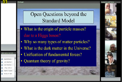
Figure 26: Videoconference with lecture by John Ellis, which he gave from his office in CERN, Switzerland, became a part of the program of XII Bled Workshop.

The ppt file of presentation is uploaded in the system in advance and then demonstrated in the central window. Video images of presenter and participants appear in the right window, while in the lower left window the list of all the attendees is given. To protect the quality of sound and record, the participants are required to switch out their audio system during presentation and to use upper left Chat window for immediate comments and urgent questions. The Chat window can be also used by participants, having no microphone, for questions and comments during Discussion. In the end of presentation the central window can be used for a whiteboard utility as well as the whole structure of windows can be changed, e.g. by making full screen the window with the images of participants of discussion.

0.70 Conclusions

The exciting experiment of VIA Discussions at Bled Workshop, the three days of permanent online transmissions and distant participation in the Gran Sasso Summer Institute on Astroparticle physics vd5VIAGS , four days of VIA interactive online transmission of series of seminars by M.Khlopov in Liege vd5VIAliege , online transmission from International Workshop on Astronomy and Relativistic Astrophysics (IWARA09, Maresias, Brazil), the stable regular weekly videoconferences with VIA lectures and the solid library of their records and presentations, creation of multi-lingual VIA Internet forum, regular basic courses and individual work on distance with students of MEPhI prove that the Scientific-Educational complex of Virtual Institute of Astroparticle physics can provide regular communications between different groups and scientists, working in different scientific fields and parts of the world, get the first-hand information on the newest scientific results, as well as to support various educational programs on distance. This activity would easily allow finding mutual interest and organizing task forces for different scientific topics of astroparticle physics and related topics. It can help in the elaboration of strategy of experimental particle, nuclear, astrophysical and cosmological studies as well as in proper analysis of experimental data. It can provide young talented people from all over the world to get the highest level education, come in direct interactive contact with the world known scientists and to find their place in the fundamental research. To conclude the VIA complex is in operation and ready for a wide use and extension of its applications.

Acknowledgements

The initial step of creation of VIA was supported by ASPERA. I am grateful to S.Katsanevas for permanent stimulating support, to P.Binetruy, J.Ellis, F.Fidecaro, M.Pohl, Y. Giraud-Heraud for help in development of the project, to K.Belotsky, A.Kirillov and K.Shibaev for assistance in educational VIA program and to C. Kouvaris, A.Mayorov and E.Soldatov for cooperation in its applications, to Z.Berezhiani and all Organizers of XIII Summer School on Astroparticle Physics in Gran Sasso, to J.-R.Cudell and all organizers of series of seminars in Liege, to Cesar Augusto Zen Vasconcellos, Rafael Martins Villas Bôas and Mario Luiz Lopes da Silva and all organizers of IWARA09 Workshop for cooperation in the use of VIA for online distant participation and to D.Rouable for help in technical realization and support of VIA complex. I express my gratitude to N.S. Mankoč Borštnik, G.Bregar, D. Lukman and all Organizers of Bled Workshop for cooperation in the exciting experiment of VIA Discussion Session at XII Bled Workshop.

References

- (1) G. F. Giudice, In Kane, Gordon (ed.), Pierce, Aaron (ed.): Perspectives on LHC physics, 155-178 (2008).
- (2) J. E. Kim, and H. P. Nilles, Phys. Lett. B138, 150 (1984).
- (3) R. Dermisek, and J. F. Gunion, Phys. Rev. Lett. 95, 041801 (2005).
- (4) M. Bastero-Gil, C. Hugonie, S. F. King, D. P. Roy, and S. Vempati, Phys. Lett. B489, 359–366 (2000).
- (5) J. F. Gunion, AIP Conf. Proc. 1030, 94–103 (2008).
- (6) C. Balazs, and D. Carter (2008).
- (7) U. Ellwanger, and C. Hugonie, Comput. Phys. Commun. 175, 290–303 (2006).
- (8) A. Djouadi, U. Ellwanger, and A. M. Teixeira, Phys. Rev. Lett. 101, 101802 (2008).
- (9) C. Hugonie, G. Belanger, and A. Pukhov, JCAP 0711, 009 (2007).
- (10) G. Belanger, F. Boudjema, C. Hugonie, A. Pukhov, and A. Semenov, JCAP 0509, 001 (2005).
- (11) D. G. Cerdeno, E. Gabrielli, D. E. Lopez-Fogliani, C. Munoz, and A. M. Teixeira, JCAP 0706, 008 (2007).
- (12) A. Djouadi, et al., JHEP 07, 002 (2008).
- (13) F. Feroz, et al., JHEP 10, 064 (2008).
- (14) R. Trotta, F. Feroz, M. P. Hobson, L. Roszkowski, and R. Ruiz de Austri, JHEP 12, 024 (2008).
- (15) S. S. AbdusSalam, B. C. Allanach, F. Quevedo, F. Feroz, and M. Hobson (2009).
- (16) U. Ellwanger, and C. Hugonie, Comput. Phys. Commun. 177, 399–407 (2007).
- (17) G. Belanger, F. Boudjema, A. Pukhov, and A. Semenov, Comput. Phys. Commun. 176, 367–382 (2007).
- (18) E. Komatsu, et al., Astrophys. J. Suppl. 180, 330–376 (2009).
- (19) Z. Ahmed, et al., Phys. Rev. Lett. 102, 011301 (2009).
- (20) F. Jegerlehner, and A. Nyffeler, arXiv:0902.3360 (2009).
- (21) E. Barberio, et al., arXiv:0808.1297 (2008).
- (22) M. Artuso, E. Barberio, and S. Stone, PMC Phys. A3, 3 (2009).
- (23) V. Barger, P. Langacker, H.-S. Lee, and G. Shaughnessy, Phys. Rev. D73, 115010 (2006).
- (24) E. A. Baltz, M. Battaglia, M. E. Peskin, and T. Wizansky, Phys. Rev. D74, 103521 (2006).
- (25) H. Baer, C. Balazs, A. Belyaev, T. Krupovnickas, and X. Tata, JHEP 06, 054 (2003).

References

- (1) D.L. Bennett and H.B. Nielsen, J. Mod. Phys A. (submitted 31 May, 1996), 1996.
- (2) D.L. Bennett and H.B. Nielsen, Intl. J. Mod. Phys., A9 (1994) 5155.
- (3) C.D. Froggatt and H.B. Nielsen, Origin of Symmetries, World Scientific Publishing Co., 1991, Singapore.
- (4) M. Nakahara, Geometry, Topology and Physics, Adam Hilger, Bristol, 1990.
- (5) B.A. Dubrovin, A.T. Fomenko and S.P. Novikov, Modern Geometry-Methods and Applications. Part II. The Geometry and Topology of Manifolds, Springer-Verlag, New York, 1984.
- (6) H.B. Nielsen, private communication.
- (7) N.S. Manton, Phys. Lett., 96B (1980) 328.

References

- (1) R. Bernabei, P. Belli, F. Cappella, R. Cerulli, F. Montecchia, F. Nozzoli, A. Incicchitti, D. Prosperi, C.J. Dai, H.H. Kuang, J.M. Ma, Z.P. Ye, ”Dark Matter particles in the galactic halo: results and implications from DAMA/NaI”, Int. J. Mod. Phys. D13 (2004) 2127-2160, astro-ph/0501412, astro-ph/0804.2738v1.
- (2) Z. Ahmed et al., A Search for WIMPs with the First Five-Tower Data from CDMS, pre-print, astro-ph/0802.3530.
- (3) S. Dodelson, Modern Cosmology, Academic Press Elsevier 2003.
- (4) C. Amsler et al., Phys. Lett. B 667, 1 (2008).
- (5) A. Borštnik Bračič, N.S. Mankoč Borštnik, ”On the origin of families of fermions and their mass matrices”, hep-ph/0512062, Phys. Rev. D 74 (2006) 073013-16.
- (6) N.S. Mankoč Borštnik, “Spin connection as a superpartner of a vielbein” Phys. Lett. B 292 (1992) 25-29, ”Unification of spin and charges”, Int. J. Theor. Phys. 40 (2001) 315-337, ”From the starting Lagrange density to the effective fields for spinors in the Approach unifying spin and charges” in the Proceedings. hep-ph/0711.4681, 94-113.
- (7) N.S. Mankoč Borštnik, “Spinor and vector representations in four dimensional Grassmann space”, J. Math. Phys. 34 (1993) 3731-3745, ”Unification of spin and charegs in Grassmann space?”, Mod. Phys. Lett. A 10 (1995) 587-595.
- (8) G. Bregar, M. Breskvar, D. Lukman, N.S. Mankoč Borštnik, ”Predictions for four families by the Approach unifying spin and charges”, New J. of Phys. 10 (2008) 093002.
- (9) N.S. Mankoč Borštnik, to be published in the Proceedings to Bled 2009 workshop, the talk can be found on www.cosmovia.org.
- (10) N.S. Mankoč Borštnik, H.B. Nielsen, ”How to generate spinor representations in any dimension in terms of projection operators”, ”How to generate families of spinor”, J. of Math. Phys. 43 (2002), (5782-5803), J. of Math. Phys. 44 (2003) 4817-4827.
- (11) G. Bregar, N.S. Mankoč Borštnik, arXiv:0812.0510 [hep-ph], 2-12, Proceedings to the workshop ”What Comes Beyond the Standard Models”, Bled July 15-25, 2008, DMFA-založništvo, Jadranska 19, 1000 Ljubljana, Slovenija, no. 1724, 1-13.
- (12) A. De Rujula, Phys. Rev. D 12 (1975) 147.
- (13) G. Bregar, M. Khlopov, N.S. Mankoč Borštnik, work in progress.
- (14) We thank cordialy R. Bernabei (in particular) and J. Filippini for very informative discussions by emails and in private communication.
- (15) V.A. Novikov, L.B. Okun,A.N. Rozanov, M.I. Vysotsky, “Extra generations and discrepancies of electroweak precision data”, Phys. Lett. B 529 (2002) 111, hep-ph/0111028, V.A. Novikov, A.N. Rozanov, M.I. Vysotsky, arXiv:0904.4570, private discussions.
- (16) A. Shchukin, talk presented at Lomonosov Conference on Elementary Particle Physics, Moscow August 19/25, 2009.
- (17) Maxim Yu. Khlopov, ”Composite dark matter from stable charged constituents”, pre-print, astro-ph/0806.3581.
- (18) M. Breskvar, D. Lukman, N.S. Mankoč Borštnik, hep-ph/0612250, p.25-50.
- (19) N. Mankoč Borštnik, M. Cvetič-Krivec, B. Golli, M. Rosina, Proc. Int. Conf on Nuclear Structure, Amsterdam (1982), Physic Letters 93B, 489-491 (1980), J. Phys. G7, 1385-1393 (1981), Rosina, Phys. Lett. 99C, 486-488 (1981).
- (20) G.D. Mack, J.F. Beacom , G. Bertone, Phys. Rev. D 76 (2007) 043523.
- (21) M. Verkerk, G. Grynberg, B. Pichard, M. Spiro, S. Zylberajch, M.E. Goldberg, P. Fayet, ”Search for superheavy hydrogen in sea watter, Phys. Rev. Lett. 8 (1992) 1116-1119.

References

- (1) E. Majorana, Nuovo Cimento 14 (1937) 171.
- (2) S. M. Bilenky and B. M. Pontekorvo, Phys. Repts 42 (1978) 224.
- (3) A. Barut and G. Ziino, Mod. Phys. Lett. A8 (1993) 1099; G. Ziino, Int. J. Mod. Phys. A11 (1996) 2081.
- (4) D. V. Ahluwalia, Int. J. Mod. Phys. A11 (1996) 1855.
- (5) P. Lounesto, Clifford Algebras and Spinors. (Cambridge University Press, 2002), Ch. 11 and 12; R. da Roacha and W. Rodrigues, Jr., Where are Elko Spinor Fields in Lounesto Spinor Field Classification? Preprint math-ph/0506075.
- (6) V. V. Dvoeglazov, Int. J. Theor. Phys. 34 (1995) 2467; Nuovo Cim. 108A (1995) 1467; Hadronic J. 20 (1997) 435; Acta Phys. Polon. B29 (1998) 619.
- (7) V. V. Dvoeglazov, Mod. Phys. Lett. A12 (1997) 2741.
- (8) M. Kirchbach, C. Compean and L. Noriega, Beta Decay with Momentum-Space Majorana Spinors. Eur. Phys. J. A22 (2004) 149.
- (9) M. Markov, ZhETF 7 (1937) 579, 603; Nucl. Phys. 55 (1964) 130.
- (10) I. M. Gelfand and M. L. Tsetlin, ZhETF 31 (1956) 1107; G. A. Sokolik, ZhETF 33 (1957) 1515.
- (11) B. Nigam and L. L. Foldy, Phys. Rev. 102 (1956) 1410.
- (12) L. H. Ryder, Quantum Field Theory. (Cambridge University Press, Cambridge, 1985).
- (13) C. Itzykson and J.-B. Zuber, Quantum Field Theory. (McGraw-Hill Book Co., 1980), p. 156.

References

- (1) V. V. Dvoeglazov, J. Phys. A33, 5011 (2000).
- (2) V. V. Dvoeglazov, Rev. Mex. Fis. Supl. 49, S1, 99 (2003) (Proceedings of the Huatulco DGFM School, 2000), math-ph/0102001.
- (3) S. Weinberg, The Quantum Theory of Fields. Vol. I. Foundations. (Cambridge University Press, Cambridge, 1995).
- (4) V. Bargmann and E. Wigner, Proc. Nat. Acad. Sci. 34, 211 (1948).
- (5) D. Luriè, Particles and Fields (Interscience Publishers, 1968).
- (6) V. V. Dvoeglazov, Hadronic J. 25, 137 (2002).
- (7) S. Weinberg, Phys. Rev. 133, B1318 (1964); ibid. 134, B882 (1964); ibid. 181, 1893 (1969).
- (8) D. L. Weaver, C. L. Hammer and R. H. Good, jr., Phys. Rev. B135, 241 (1964); R. H. Tucker and C. L. Hammer, Phys. Rev. D3, 2448 (1971).
- (9) V. V. Dvoeglazov, Hadronic J., 26, 299 (2003), hep-th/0208159.
- (10) V. V. Dvoeglazov, Helv. Phys. Acta 70, 677; ibid. 686; ibid. 697 (1997); Ann. Fond. Broglie 23, 116 (1998); Int. J. Theor. Phys. 37, 1915 (1998).
- (11) V. V. Dvoeglazov, Phys. Scripta 64, 201 (2001).
- (12) H. M. Rück y W. Greiner, J. Phys. G: Nucl. Phys. 3, 657 (1977).
- (13) V. B. Berestetskiĭ, E. M. Lifshitz and L. P. Pitaevskiĭ, Quantum Electrodynamics. (Pergamon Press, 1982, translated from the Russian), p.16.
- (14) V. I. Ogievetskiĭ and I. V. Polubarinov, Yadern. Fiz. 4, 216 (1966) [English translation: Sov. J. Nucl. Phys. 4, 156 (1967)].
- (15) K. Hayashi, Phys. Lett. B44, 497 (1973).
- (16) M. Kalb and P. Ramond, Phys. Rev. D9, 2273 (1974).
- (17) V. V. Dvoeglazov, Int. J. Theor. Phys. 43, 1287 (2004), math-ph/0309002.
- (18) S. I. Kruglov and A. F. Radyuk, Vestzi AN BSSR: Fiz. Mat., No. 2, 48 (1979); S. I. Kruglov, Vestzi AN BSSR, No. 4, 87 (1982); Hadronic J. 24, 167 (2001); Ann. Fond. Broglie 26, 725 (2001); Int. J. Theor. Phys. 41, 653 (2002); Int. J. Mod. Phys. A16, 4925 (2001).
- (19) C. Itzykson and J.-B. Zuber, Quantum Field Theory (McGraw-Hill Book Co., 1980).
- (20) L. Ryder, Quantum Field Theory (Cambridge University Press, Cambridge, 1985).
- (21) N. N. Bogoliubov and D. V. Shirkov, Introduction to the theory of Quantized Fields (Wiley, 1980), p.90 of the Russian edition.
- (22) V. V. Dvoeglazov, Adv. Appl. Clifford Algebras, 10, 7 (2000), math-ph/9805017.
- (23) H. Snyder: Phys. Rev. 71, 38 (1947); ibid. 72, 68 (1947).
- (24) S. Doplicher et al.: Phys. Lett. B331, 39 (1994); S. Majid and H. Ruegg: Phys. Lett. B334, 348 (1994); J. Lukierski, H. Ruegg and W. J. Zakrzewski: Ann. Phys. 243, 90 (1995); N. Seiberg and E. Witten: JHEP 9909, 032 (1999), hep-th/9908142; I. F. Riad and M. M. Sheikh-Jabbari: JHEP 08, 045 (2000), hep-th/0008132; M. M. Sheikh-Jabbari: Phys. Rev. Lett. 84, 5265 (2000), hep-th/0001167; J. Madore et al.: Eur. Phys. J. C16, 161 (2000); S. I. Kruglov: Ann. Fond. Broglie 27, 343 (2002).
- (25) F. Dyson: Am. J. Phys. 58, 209 (1990); S. Tanimura: Ann. Phys. 220, 229 (1992); see also many subsequent comments on these works.
- (26) K. R. Brownstein: Am. J. Phys. 67, 639 (1999); J. D. Jackson: hep-ph/0203076, L. Škovrlj and T. Ivezić: hep-ph/0203116; V. Dvoeglazov, Spacetime and Substance: 3, 125 (2002).
- (27) A. E. Chubykalo, R. A. Flores and J. A. Pérez: in Proc. of the Internatinal Workshop “Lorentz Group, CPT and Neutrinos”, Zacatecas, México, June 1999. Eds. V. V. Dvoeglazov et al. World Scientific, 2000, 384-396; A. E. Chubykalo and R. A. Flores: Hadronic J. 25, 159 (2002).
- (28) L. D. Landau and E. M. Lifshitz: The Classical Theory of Fields. 4th revised English ed. Translated from the 6th Russian edition. Pergamon Press, 1979. 402p., p. 63.
- (29) V. V. Dvoeglazov, Proceedings of the 11th Workshop ”What Comes Beyond the Standard Models?” Bled. Slovenia, July 2008, arXiv:0711.4681 .
- (30) A. Kempf, G. Mangano and R. B. Mann: Phys. Rev. D52 , 1108 (1995); G. Amelino-Camelia: Nature 408, 661 (2000); gr-qc/0012051; hep-th/0012238; gr-qc/0106004; J. Kowalski-Glikman: hep-th/0102098; G. Amelino-Camelia and M. Arzano: hep-th/0105120; N. R. Bruno, G. Amelino-Camelia and J. Kowalski-Glikman: hep-th/0107039.
- (31) V. V. Dvoeglazov: Rev. Mex. Fis. Supl. 49, 99 (2003) (Proceedings of the DGFM-SMF School, Huatulco, 2000).
- (32) R. A. Berg: Nuovo Cimento 42A, 148 (1966); V. V. Dvoeglazov: ibid. A108, 1467 (1995).

References

- (1) S. Weinberg, Phys. Rev. Lett.29, 388(1972); H. Georgi and S.L. Glashow, Phys. Rev. D 7, 2457(1973); R.N. Mohapatra, Phys. Rev. D 9, 3461(1974); S.M. Barr and A. Zee, Phys. Rev. D 15, 2652(1977); H. Georgi, ”Fermion Masses in Unified models”, in First Workshop in Grand Unification, ed. P.H. Frampton, S.L. Glashow, and A. Yildiz(1980, Math Sci Press, Brookline, MA); S.M. Barr ,Phys. Rev. D 21, 1424(1980); R. Barbieri and D.V. Nanopoulos, Phys. Lett. B 95, 43(1980); S.M. Barr ,Phys. Rev. D 24, 1895(1981); L.E. Ibanez, Phys. Lett. B 177, 403(1982); B.S. Balakrishna, A.L. Kagan and R.N. Mohapatra, Phys. Lett. B 205, 345(1988); B.S. Balakrishna, Phys. Rev. Lett. 60, 1602(1988); K.S. Babu and E. Ma, Mod. Phys. Lett. A 4 , 1975(1989); H.P. Nilles, M. Olechowski and S. Pokorski, Phys. Lett. B 248, 378(1990); R. Rattazzi, Z. Phys.C 52, 575(1991); K.S. Babu and R.N. Mohapatra, Phys. Rev. Lett. 64, 2747(1990); X.G. He, R.R. Volkas, and D.D. Wu, Phys. Rev. D 41, 1630(1990); Ernest Ma, Phys. Rev. Lett. 64 (1990) 2866. B.A. Dobrescu and P.J. Fox, JHEP 0808, 100(2008); S.M. Barr, Phys. Rev. D 76, 105024(2007); S.M. Barr and A. Khan, Phys. Rev. D 79, 115005(2009);
- (2) Sandip Pakvasa and Hirotaka Sugawara, Phys. Lett. B73, 61 (1978); Y. Yamanaka, H. Sugawara, and S. Pakvasa, Phys. Rev. D 25, 1895 (1982); K. S. Babu and X.G. He, ibid. 36, 3484 (1987) ; Ernest Ma, Phys. Rev. Lett. B 62, 61 (1989).
- (3) A. Davidson, M. Koca, and K. C. Wali, Phys. Rev. Lett. B 43, 92 (1979), Phys. Rev. D 20, 1195 (1979); C. D. Froggatt and H. B. Nielsen, Nucl. Phys. B 147, 277 (1979); A. Sirlin, Phys. Rev. D 22, 971 (1980); A. Davidson and K. C. Wali, ibid. 21, 787 (1980) .
- (4) X.G. He, R. R: Volkas, and D. D. Wu, Phys. Rev. D 41, 1630 (1990); Ernest Ma, Phys. Rev. Lett. 64, 2866 (1990).
- (5) E. Garcia, A. Hernandez-Galeana, D. Jaramillo, W. A. Ponce and A. Zepeda, Revista Mexicana de Fisica Vol. 48(1), 32 (2002), hep-ph/0006093; E. Garcia, A. Hernandez-Galeana, A. Vargas and A. Zepeda, hep-ph/0203249.
- (6) For reviews, see E. H. Simmons, in Proc. of the APS/DPF/DPB summer study on the future of Particle Physics (Snowmass 2001) ed. N. Graf, eConf C010630, P110 (2001) C. T. Hill and E. H. Simmons, Phys. Rept. 381, 235 (2003). T. Appelquist, M. Piai and R. Shrock, Phys. lett. B593, 175 (2004), Phys. Rev. D69, 015002 (2004); T. Appelquist, R. Shrock, Phys. Rev. Lett. 90, 201801 (2003).
-
(7)
Some references on family symmetry models are
M. Bowick and P. Ramond, Phys. Lett. B 103, 338 (1981); D. R. T. Jones, G. L. Kane, and J. P. Leveille, Nucl. Phys. B198, 45 (1982); Z. G. Berezhiani, Phys. Lett. B 150, 177 (1985); Z. G. Berezhiani and M. Y. Khlopov, Yad. Fiz. 51, 1157 (1990) [Sov. J. Nucl. Phys. 51, 739 (1990)]; Z. Berezhiani and A. Rossi, Nucl. Phys. B594, 113 (2001); A. Masiero, M. Piai, A. Romanino, and L. Silvestrini, Phys. Rev. D 64, 075005 (2001); S. F. King and G. G. Ross, Phys. Lett. B 520, 243 (2001); 574, 239 (2003); G. G. Ross, L. Velasco-Sevilla, and O. Vives, Nucl. Phys. B692, 50 (2004); A. Hernandez-Galeana, Rev. Mex. Fis. 50, 522 (2004); I. de Medeiros Varzielas and G. G. Ross, Nucl. Phys. B733, 31 (2006); I. de Medeiros Varzielas, S. F. King, and G. G. Ross, Phys. Lett. B 644, 153 (2007); T. Appelquist, Y. Bai, and M. Piai, Phys. Lett. B 637, 245 (2006); T. Appelquist, Y. Bai, and M. Piai, Phys. Rev. D 74, 076001 (2006). -
(8)
For review and some recent works see for example:
B. Holdom, W.S. Hou, T. Hurth, M. Mangano, S. Sultansoy and G. Unel, ”Beyond the 3-generation SM in the LHC era” Workshop, CERN, September 4-5, 2008; arXiv:0904.4698 and references therein, A.B. Bracic and N.S.M. Borstnik, Phys. Rev. D74, 073013 (2006), and talk by N.S.M. Borštnik at this Workshop, K.M. Belotsky et al, Grav. Cosmol. 11, 3 (2005); talk by M. Khlopov at this Workshop. - (9) A. Hernandez-Galeana, Phys.Rev.D 76, 093006 (2007).
- (10) C. Amsler et al., Particle Data Group, Phys. Lett. B 667, 1(2008).

References

- (1) M.Yu. Khlopov Cosmoparticle physics (World Scientific, Singapore, 1999).
- (2) M.Yu. Khlopov in Cosmion-94, Eds. M.Yu.Khlopov et al. (Editions frontieres, 1996) P. 67; M. Y. Khlopov in hep-ph/0612250 , p 51.
- (3) M. Y. Khlopov in arXiv:0711.4681, p. 114; M. Y. Khlopov and N. S. Mankoc-Borstnik, ibid, p. 195.
- (4) S. L. Glashow, arXiv:hep-ph/0504287.
- (5) D. Fargion and M. Khlopov, arXiv:hep-ph/0507087.
- (6) M.Yu. Khlopov, JETP Lett. 83, 1 (2006).
- (7) K. Belotsky et al, arXiv:astro-ph/0602261. K. Belotsky et al, Gravitation and Cosmology 12, 1 (2006); K. Belotsky et al, arXiv:0806.1067 [astro-ph].
- (8) M. Y. Khlopov, arXiv:astro-ph/0607048.
- (9) K.M.Belotsky et al, Gravitation and Cosmology 11, 3 (2005)
- (10) C. A. Stephan, arXiv:hep-th/0509213.
- (11) D. Fargion et al, Class. Quantum Grav. 23, 7305 (2006); M. Y. Khlopov and C. A. Stephan, arXiv:astro-ph/0603187.
- (12) A. Connes Noncommutative Geometry (Academic Press, London and San Diego, 1994). M. Y. Khlopov and C. A. Stephan, arXiv:astro-ph/0603187.
- (13) M. Y. Khlopov and C. Kouvaris, Phys. Rev. D 77, 065002 (2008).
- (14) F. Sannino and K. Tuominen, Phys. Rev. D 71, 051901 (2005); D. K. Hong et al, Phys. Lett. B 597, 89 (2004); D. D. Dietrich et al, Phys. Rev. D 72, 055001 (2005); D. D. Dietrich et al, arXiv:hep-ph/0510217; S. B. Gudnason et al, Phys. Rev. D 73, 115003 (2006); S. B. Gudnason et al, Phys. Rev. D 74, 095008 (2006).
- (15) N.S. Mankoč Borštnik, This Volume; A. Borštnik Bračič, N.S. Mankoč Borštnik, Phys. Rev. D 74, 073013 (2006); N.S. Mankoč Borštnik, Mod. Phys. Lett. A 10, 587 (1995); N.S. Mankoč Borštnik, Int. J. Theor. Phys. 40, 315 (2001); G. Bregar, M. Breskvar, D. Lukman, N.S. Mankoč Borštnik, New J. of Phys. 10, 093002 (2008).
- (16) M. Y. Khlopov, arXiv:0806.3581 [astro-ph].
- (17) C. B. Dover et al, Phys. Rev. Lett. 42, 1117 (1979); S. Wolfram, Phys. Lett. B 82, 65 (1979); G. D. Starkman et al, Phys. Rev. D 41, 3594 (1990); D. Javorsek et al, Phys. Rev. Lett. 87, 231804 (2001); S. Mitra, Phys. Rev. D 70, 103517 (2004); G. D. Mack et al, Phys. Rev. D 76, 043523 (2007);
- (18) B. D. Wandelt et al., arXiv:astro-ph/0006344; P. C. McGuire and P. J. Steinhardt, arXiv:astro-ph/0105567; G. Zaharijas and G. R. Farrar, Phys. Rev. D 72, 083502 (2005)
- (19) M. Y. Khlopov, arXiv:0801.0167 [astro-ph]; M. Y. Khlopov, arXiv:0801.0169 [astro-ph].
- (20) M. Y. Khlopov and C. Kouvaris, Phys. Rev. D 78, 065040 (2008)
- (21) R. Bernabei et al., Rivista Nuovo Cimento 26, 1 (2003)
- (22) R. Bernabei et al. [DAMA Collaboration],Eur.Phys.J C56, 333 (2008) arXiv:0804.2741 [astro-ph].
- (23) D. McCammon et al, Nucl. Instrum. Methods A 370, 266 (1996); D. McCammon et al, Astrophys. J. 576, 188 (2002).
- (24) K. Belotsky et al, arXiv:astro-ph/0606350.
- (25) D. S. Akerib et al. [CDMS Collaboration], Phys. Rev. Lett. 96, 011302 (2006); Z. Ahmed et al. [CDMS Collaboration], arXiv:0802.3530 [astro-ph]. N. Mirabolfathi et al. [CDMS Collaboration], Nucl. Instrum. Methods A 559, 417 (2006);
- (26) V. B. Berestecky, E. M. Lifshitz, L. P. Pitaevsky Quantum Electrodynamics (Nauka, Moscow, 1989).
- (27) O. Kamaev, for the CDMS Collaboration, arXiv:0910.3005 [hep-ex].
- (28) F. Petriello and K. M. Zurek, JHEP 0809, 047 (2008); R. Foot, Phys. Rev. D 78, 043529 (2008); J. L. Feng, J. Kumar and L. E. Strigari, arXiv:0806.3746 [hep-ph]; J. L. Feng, J. Kumar, J. Learned and L. E. Strigari, arXiv:0808.4151 [hep-ph]; E. M. Drobyshevski, arXiv:0811.0151 [astro-ph].
- (29) G. B. Gelmini, arXiv:0810.3733 [hep-ph].
- (30) L. D. Landau, E. M. Lifshitz Quantum Mechanics: Non-Relativistic Theory (Fizmatlit, Moscow, 2004).

References

- (1) Random Dynamics Homepage, http://www.nbi.dk/ kleppe/random/qa/qa.html, Random Dynamics references, http://www.nbi.dk/ kleppe/random/qa/rref.html
- (2) B. Meltzer (translation) and R. B. Braithwaite (Introduction), 1962. On Formally Undecidable Propositions of Principia Mathematica and Related Systems, Dover Publications, New York (Dover edition 1992, Stephen Hawking editor, 2005. God Created the Integers: The Mathematical Breakthroughs That Changed History, Running Press, Philadelphia, ISBN 0-7624-1922-9.
- (3) Gregory Chaitin, Information-Theoretic Incompleteness, (World Scientific, 1992), The Limits of Mathematics, (Springer-Verlag 1998)
- (4) Stephen Wolfram, A New Kind of Science, http://www.wolframscience.com
- (5) Grigory E. Volovik, The Universe in a Helium Droplet (The International Series of Monographs on Physics, 117)

References

- (1) E. Witten, Nucl. Phys. B 186 (1981) 412; Princeton Technical Rep. PRINT -83-1056, October 1983.
- (2) N. S. Mankoč Borštnik, Phys. Lett. B 292 (1992) 25.
- (3) N. S. Mankoč Borštnik, J. Math. Phys. 34 (1993) 3731.
- (4) N. S. Mankoč Borštnik, Int. J. Theor. Phys. 40 315 (2001).
- (5) N. S. Mankoč Borštnik, Modern Phys. Lett. A 10 (1995) 587.
- (6) A. Borštnik, N. S. Mankoč Borštnik, hep-ph/0401043, hep-ph/0401055, hep-ph/0301029.
- (7) A. Borštnik Bračič, N.S. Mankoč Borštnik, Phys. Rev. D 74 (2006)073013, hep-ph/0512062.
- (8) G. Bregar, M. Breskvar, D. Lukman, N.S. Mankoč Borštnik, hep-ph/0711.4681.
- (9) G. Bregar, M. Breskvar, D. Lukman, N.S. Mankoč Borštnik, New J. of Phys. 10 (2008) 093002, hep-ph/0606159, hep/ph-07082846.
- (10) N. S. Mankoč Borštnik, H. B. Nielsen, Phys. Lett. B 633 (2006) 771-775, hep-th/0311037, hep-th/0509101.
- (11) N. S. Mankoč Borštnik, H. B. Nielsen, Phys. Lett. B 644 (2007)198-202, hep-th/0608006.
- (12) N. S. Mankoč Borštnik, H. B. Nielsen, Phys. Lett. B 10.1016 (2008).
- (13) N. S. Mankoč Borštnik, H. B. Nielsen, D. Lukman, hep-ph/0412208.
- (14) S. Deser, gr-qc/9512022.
- (15) N. S. Mankoč Borštnik, H. B. Nielsen, J. of Math. Phys. 43 (2002) 5782, hep-th/0111257.
- (16) N. S. Mankoč Borštnik, H. B. Nielsen, J. of Math. Phys. 44 (2003) 4817, hep-th/0303224.
- (17) N. S. Mankoč Borštnik, H. B. Nielsen, Phys. Lett. B 633 (2006) 771, hep-th/0311037, hep-th/0509101, Phys. Lett. B 10.1016 (2008), Phys. Lett. B 644 (2007)198-202, hep-th/0608006.
- (18) M. Breskvar, D. Lukman, N.S. Mankoč Borštnik, hep-ph/0612250, p.25-50.
- (19) M. Blagojević, Gravitation and gauge symmetries (I. of Phys. Pub, ISBN 0750307676, 2001).

References

- (1) N.S. Mankoč Borštnik, Phys. Lett. B 292 (1992) 25-29, J. Math. Phys. 34 (1993) 3731-3745, Modern Phys. Lett. A 10 (1995) 587-595, Int. J. Theor. Phys. 40 (2001) 315-337.
- (2) A. Borštnik Bračič, N.S. Mankoč Borštnik, Phys Rev. D 74 (2006) 073013-16.
- (3) G. Bregar, M. Breskvar, D. Lukman, N.S. Mankoč Borštnik, New J. of Phys. 10 (2008) 093002.
- (4) N. S. Mankoč Borštnik, hep-ph/0711.4681, 94-113.
- (5) N.S. Mankoč Borštnik, H.B. Nielsen, J. of Math. Phys. 43 (2002), (5782-5803), J. of Math. Phys. 44 (2003) 4817-4827.
- (6) D. Lukman, N.S. Mankoč Borštnik, H.B. Nielsen, this proceedings.
- (7) D. Lukman, N.S. Mankoč Borštnik, H.B. Nielsen, arxiv:0812.0510[hep-ph],44-55.
- (8) N.S. Mankoč Borštnik, H.B. Nielsen, Phys. Lett. B 633 771 (2006), hep-th/0311037, hep-th/0509101; Phys. Lett. B 10.1016 (2008), the talk in this proceedings. Phys. Lett. B 644 (2007)198-202, hep-th/0608006.
- (9) M. Breskvar, D. Lukman, N.S. Mankoč Borštnik, hep-ph/0612250, p.25-50.
- (10) G. Bregar, N.S. Mankoč Borštnik, Phys. Rev. D 80, 083534 (2009), astro-ph¿arXiv: 0811.4106, arXiv:0812.0510 [hep-ph], 2-12,
- (11) G. Bregar, N.S. Mankoč Borštnik, in this proceedings.
- (12) R. Bernabei at al, Int.J.Mod.Phys. D13 (2004) 2127-2160, astro-ph/0501412, astro-ph/0804.2738v1.
- (13) Z. Ahmed et al., pre-print, astro-ph/0802.3530.
- (14) C. Amsler et al., Physics Letters B667, 1 (2008).
- (15) S. Dodelson, Modern Cosmology, Academic Press Elsevier 2003.
- (16) N.S. Mankoč Borštnik, H. B. Nielsen, Phys. Lett. B 633 (2006) 771-775, hep-th/0311037, hep-th/0509101.
- (17) N. S. Mankoč Borštnik, H. B. Nielsen, Phys. Lett. B 644 (2007)198-202, hep-th/0608006.
- (18) N.S. Mankoč Borštnik, H. B. Nielsen, Phys. Lett. B, Phys. Lett. B 10.1016 (2008) 10.1016 (2008).
- (19) E. Witten, Nucl. Phys. B 186 (1981) 412; Princeton Technical Rep. PRINT -83-1056, October 1983.
- (20) G. Bregar, M. Khlopov, N.S. Mankoč Borštnik, work in progress.
- (21) We thank cordially R. Bernabei (in particular) and J. Filippini for very informative discussions by emails and in private communication.
- (22) V.A. Novikov, L.B. Okun,A.N. Royanov, M.I. Vysotsky, Phys. Lett. B 529(2002) 111, hep-ph/0111028.
- (23) Maxim Yu. Khlopov, pre-print, astro-ph/0806.3581.

References

- (1) Borstnik, Norma Mankoc, Holger Bech Nielsen, Colin D. Froggatt, Dragan Lukman (2004), ”Proceedings to the 7th Workshop ’What comes beyond the Standard models’, July 19 – July 31. 2004, Bled, Slovenia”, Bled Workshops in Physics, Volume 5, No. 2, December.
- (2) Borstnik, Norma Mankoc, Holger Bech Nielsen, Colin D. Froggatt, Dragan Lukman (2005), ”Proceedings to the 8th Workshop ’What comes beyond the Standard models’, July 19 – July 29. 2005, Bled, Slovenia”, Bled Workshops in Physics, Volume 6, No. 2, December.
- (3) Borstnik, Norma Mankoc, Holger Bech Nielsen, Colin D. Froggatt, Dragan Lukman (2006), ”Proceedings to the 9th Workshop ’What comes beyond the Standard models’, July 19 – July 29. 2006, Bled, Slovenia”, Bled Workshops in Physics, Volume 7, No. 2, December.
- (4) Borstnik, Norma Mankoc, Holger Bech Nielsen, Colin D. Froggatt, Dragan Lukman (2007), ”Proceedings to the 10th Workshop ’What comes beyond the Standard models’, July 17 – July 27. 2006, Bled, Slovenia”, Bled Workshops in Physics, Volume 8, No. 2, December.
- (5) Borstnik, Norma Mankoc, Holger Bech Nielsen, Colin D. Froggatt, Dragan Lukman (2007), ”Proceedings to the 11th Workshop ’What Comes Beyond the Standard Models’, 15–25 July 2008, Bled, Slovenia”, Bled Workshops in Physics, Volume 9, No. 2 (December 2008), p. 56-64.
- (6) Merzbacher, Eugen (1967), Quantum Mechanics (New York: John Wiley and Sons, Inc.).
- (7) Mirman, R. (1995a), Group Theory: An Intuitive Approach (Singapore: World Scientific Publishing Co.).
- (8) Mirman, R. (1995b), Group Theoretical Foundations of Quantum Mechanics (Commack, NY: Nova Science Publishers, Inc.; republished by Backinprint.com).
- (9) Mirman, R. (1995c), Massless Representations of the Poincaré Group, electromagnetism, gravitation, quantum mechanics, geometry (Commack, NY: Nova Science Publishers, Inc.; republished by Backinprint.com).
- (10) Mirman, R. (1999), Point Groups, Space Groups, Crystals, Molecules (Singapore: World Scientific Publishing Co.).
- (11) Mirman, R. (2001a), Quantum Mechanics, Quantum Field Theory: geometry, language, logic (Huntington, NY: Nova Science Publishers, Inc.; republished by Backinprint.com).
- (12) Mirman, R. (2001b), Quantum Field Theory, Conformal Group Theory, Conformal Field Theory: Mathematical and conceptual foundations, physical and geometrical applications (Huntington, NY: Nova Science Publishers, Inc.; republished by Backinprint.com).
- (13) Mirman, R. (2004a), Geometry Decides Gravity, Demanding General Relativity — It Is Thus the Quantum Theory of Gravity, in rm1con-nmb , p. 84-93.
- (14) Mirman, R. (2004b), Physics Would Be Impossible in Any Dimension But 3+1 — There Could Be Only Empty Universes, in rm1con-nmb , p. 94-101.
- (15) Mirman, R. (2004c), Conservation of Energy Prohibits Proton Decay, in rm1con-nmb , p. 102-106.
- (16) Mirman, R. (2005), Are there Interesting Problems That Could Increase Understanding of Physics and Mathematics? in rm1con-nm2 , p. 72-78.
- (17) Mirman, R. (2006), How Can Group Theory be Generalized so Perhaps Providing Further Information About Our Universe? in rm1con-nm3 , p. 80-86.
- (18) Mirman, R. Mass Spectra are Inherent in Geometry: an Analysis Using the Only Conformal Group Allowing a Universe, in rm1con-nm4 , p. 136-143.
- (19) Mirman, R., Some Obvious Matters of Physics That Are Not Obvious, in rm1con-nm5 , p. 56-64.
- (20) Mirman, R. (2006), Our Almost Impossible Universe: Why the laws of nature make the existence of humans extraordinarily unlikely (Lincoln, NE: iUniverse, Inc.)
- (21) Mirman, R. (2006), impunv.wordpress.com; impunv.blogspot.com

References

- (1) G. Bregar, J. Filippini, M. Khlopov, N. S. Mankoc-Borstnik, A. Mayorov and E. Soldatov, In *Bled 2008, What comes beyond the standard models* 67-71.
- (2) N.S. Mankoč Borštnik, ”Offering the mechanism for generating families the Approach unifying spin and charges predicts new families”, p.119 in this proceedings
- (3) A. Borštnik Bračič, N.S. Mankoč Borštnik, ”On the origin of families of fermions and their mass matrices”, hep-ph/0512062, Phys. Rev. D 74 (2006) 073013-16.
- (4) G. Bregar, M. Breskvar, D. Lukman, N.S. Mankoč Borštnik, New J. of Phys. 10 (2008) 093002.
- (5) G. Bregar, N.S. Mankoč Borštnik, Phys. Rev. D 80 (2009) 083534, the talk in this proceedings, p. 19, discussions in the discussion section.

References

- (1) N. S. Mankoč Borštnik, H. B. Nielsen, Phys. Lett. B 633 (2006) 771-775, hep-th/0311037, hep-th/0509101.
- (2) N. S. Mankoč Borštnik, H. B. Nielsen, Phys. Lett. B 10.1016 (2008).

References

- (1) N.S. Mankoč Borštnik, talk in this proceedings, p.119 and the references therein.
- (2) A. Borštnik Bračič, N.S. Mankoč Borštnik, ”On the origin of families of fermions and their mass matrices”, hep-ph/0512062, Phys. Rev. D 74 (2006) 073013-16 and references therein.
- (3) G. Bregar, M. Breskvar, D. Lukman, N.S. Mankoč Borštnik, ”Predictions for four families by the Approach unifying spin and charges”, New J. of Phys. 10 (2008) 093002.
- (4) G. Bregar, N.S. Mankoč Borštnik, Phys. Rev. D 80, 083534 (2009), and the talk appearing in this proceedings, p. 19.
- (5) Dolgov, A. D. 2002, Phys. Rep., 370, 333 (arXiv:hep-ph/0202122)
- (6) Maxim Yu. Khlopov, ”Composite dark matter from stable charged constituents”, pre-print, astro-ph/0806.3581.
- (7) E. Elfgren and S. Fredriksson, “Mass limits for heavy neutrinos,” arXiv:0710.3893 [astro-ph].

References

- (1) N.S. Mankoč Borštnik, talk in this proceedings, p.119 and the references therein.
- (2) A. Borštnik Bračič, N.S. Mankoč Borštnik, ”On the origin of families of fermions and their mass matrices”, hep-ph/0512062, Phys. Rev. D 74 (2006) 073013-16 and references therein.
- (3) G. Bregar, M. Breskvar, D. Lukman, N.S. Mankoč Borštnik, ”Predictions for four families by the Approach unifying spin and charges”, New J. of Phys. 10 (2008) 093002.
- (4) G. Bregar, N.S. Mankoč Borštnik, Phys. Rev. D 80, 083534 (2009), and the talk appearing in this proceedings, p. 19.
- (5) D. Fargion et al., JETP Lett. 69, 434 (1999); arXiv:astro-ph-9903086; K.M.Belotsky et al, Gravitation and Cosmology 6 Supplement, 140 (2000); K.M.Belotsky et al, “May Heavy neutrinos solve underground and cosmic ray puzzles?,” Phys.Atom.Nucl. 65, 2008 147 K.M.Belotsky et al, Gravitation and Cosmology 11, (2005), 16 and references therein.
- (6) K.M.Belotsky, D.Fargion, M.Yu.Khlopov, R.Konoplich, M.G.Ryskin and K.I.Shibaev, Gravitation and Cosmology 11 (2005) 3 . K. Belotsky, M. Khlopov and K. Shibaev, “Stable quarks of the 4th family?,”Invited contribution to the book ”The Physics of Quarks: New Research.” NOVA, 2008, arXiv:0806.1067 [astro-ph] and references therein.
- (7) D. Fargion and M. Khlopov, “Tera-leptons shadows over sinister Universe,” arXiv:hep-ph/0507087.
- (8) D. Fargion et al,“Cold dark matter by heavy double charged leptons?, Class. Quantum Grav. 23, (2006) 7305.
- (9) M.Yu. Khlopov, JETP Lett. 83 (2006) 1; K. Belotsky et al,“Composite dark matter and its charged constituents,” , Gravitation and Cosmology 12 (2006) 1.
- (10) M. Y. Khlopov and C. Kouvaris, “Strong Interactive Massive Particles from a Strong Coupled Theory,” Phys. Rev. D 77 2008 065002. M. Y. Khlopov and C. Kouvaris, “Composite dark matter from a model with composite Higgs boson,” Phys. Rev. D 78 (2008) 065040
- (11) M. Yu. Khlopov, A. G. Mayorov, E.Yu. Soldatov, this Volume.
- (12) O. Kamaev for the CDMS Collaboration, arXiv:0910.3005 [hep-ex].

References

- (1) See for instance: A. Hernandez-Galeana, Phys. Rev. D 76 (2007) 093006, arXiv: 0710.2834

References

- (1) http://www.aspera-eu.org/
- (2) M.Yu. Khlopov: Cosmoparticle physics, World Scientific, New York -London-Hong Kong - Singapore, 1999
- (3) M. Y. Khlopov, arXiv:0801.0376 [astro-ph].
- (4) http://www.cosmovia.org/
- (5) M. Y. Khlopov, In *Bled 2008, What comes beyond the standard models* 81-86
- (6) G. Bregar, J. Filippini, M. Khlopov, N. S. Mankoc-Borstnik, A. Mayorov and E. Soldatov, In *Bled 2008, What comes beyond the standard models* 67-71
- (7) In http://www.cosmovia.org/ Previous - Conferences - XII Bled Workshop
- (8) G. Bregar and N.S. Mankoč Borštnik, This Volume; M.Yu.Khlopov, A.Mayorov and E.Soldatov, This Volume
- (9) In http://www.cosmovia.org/ Previous - Conferences - Gran Sasso
- (10) In http://www.cosmovia.org/ Previous - Conferences - Liege
Blejske Delavnice Iz Fizike, Letnik 10, št. 2, ISSN 1580-4992
Bled Workshops in Physics, Vol. 10, No. 2
Zbornik 12. delavnice ‘What Comes Beyond the Standard Models’, Bled, 14. – 24. julij 2009
Proceedings to the 12th workshop ’What Comes Beyond the Standard Models’, Bled, July 14.–24., 2009
Uredili Norma Susana Mankoč Borštnik, Holger Bech Nielsen in Dragan Lukman
Publikacijo sofinancira Javna agencija za knjigo Republike Slovenije
Brezplačni izvod za udeležence
Tehnični urednik Vladimir Bensa
Založilo: DMFA – založništvo, Jadranska 19, 1000 Ljubljana, Slovenija
Natisnila ALFAGRAF TRADE v nakladi 150 izvodov
Publikacija DMFA številka 1762