Entanglement of mechanical oscillators coupled to a non-equilibrium environment
Abstract
Recent experiments aim at cooling nanomechanical resonators to the ground state by coupling them to non-equilibrium environments in order to observe quantum effects such as entanglement. This raises the general question of how such environments affect entanglement. Here we show that there is an optimal dissipation strength for which the entanglement between two coupled oscillators is maximized. Our results are established with the help of a general framework of exact quantum Langevin equations valid for arbitrary bath spectra, in and out of equilibrium. We point out why the commonly employed Lindblad approach fails to give even a qualitatively correct picture.
pacs:
03.65.Yz 03.67.Bg 07.10.Cm 42.50.LcI 1. Introduction
Entanglement 1935_Schroedinger constitutes a cornerstone of quantum mechanics and is a major subject of present-day research 2009_Horodecki_RMPQuEntanglement . Whether it persists and can be observed in systems comprising macroscopic bodies has been a hotly debated topic since the early days of quantum mechanics. The ground state of two interacting quantum systems will generically be entangled. Thus, one could naively expect that it is sufficient to simply cool two interacting, macroscopic bodies to their ground states and thereby prepare an entangled state. However, when coupling to a dissipative bath – as is of course necessary for cooling – entanglement may be destroyed, as explored in a number of works, e.g., Examples_EntanglementDissipation . A slate of recent experiments has now brought a new aspect into focus: A non-equilibrium environment, consisting of either a driven optical cavity Examples_Optomechanics , a superconducting microwave resonator Examples_Microwave or a superconducting single electron transistor 2006_Naik_CoolingNanomechResonator , can be employed to cool the motion of mechanical resonators down to the ground state. The advances in this field may ultimately enable tests of quantum mechanics in an entirely new regime 2005_Schwab and to observe entanglement of massive objects OptomechanicsEntanglement ; 2008_Hartmann . Still it remains to resolve the issue of how the dissipative coupling to the non-equilibrium bath affects entanglement.
In the present work, we demonstrate a non-monotonic dependence of entanglement between two oscillators on the coupling strength to the non-equilibrium environment and show that there is an optimal value for the coupling to the bath. Below this value, entanglement is diminished by thermal fluctuations, and above this value, it is lost through dissipation. The striking behavior found here is missed entirely by the commonly employed Lindblad approach to dissipative dynamics.
In order to obtain an exact description, we develop a general framework based on quantum Langevin equations, which allows us to analyze the entanglement between harmonic oscillators in the presence of coupling to a linear bath of arbitrary spectral density. First, we exploit this scheme to show that even in equilibrium there are effects likely to be missed by simpler approaches. For example, the minimum coupling strength needed for entanglement depends logarithmically on the cutoff frequency for the most important case of an Ohmic bath spectrum. For the case of a non-equilibrium bath, we illustrate the generic behavior in a concrete example of two mechanical resonators inside an optical cavity, being cooled by the optomechanical interaction with the light field circulating in the cavity.
II 2. Model
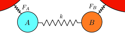
We consider two coupled oscillators with masses and frequencies , cf. Fig. 1. In terms of their positions and momenta, and the Hamiltonian reads , with a coupling spring constant . Moreover, we assume the oscillators to be subject to fluctuating quantum forces , which are possibly correlated, and which derive from a bath of harmonic oscillators, with . They will be characterized by their spectra as specified below.
If the state of the environment is Gaussian, the oscillators also end up in a Gaussian state, which is fully described by the covariance matrix . Here in steady state, and is the system’s density matrix. As a measure of the entanglement between the oscillators, the logarithmic negativity 1999_Eisert_EntanglementMeasures_JModOpt ; 2000_Simon ; 2002_Vidal_Entanglement is calculated as where for and otherwise, and where are the symplectic eigenvalues of the partially transposed covariance matrix 2002_Vidal_Entanglement .
For later use, and in order to fix the notation it will be convenient to consider first the simple example of two identical oscillators ( ) at thermal equilibrium and assume the coupling to the environment to be negligible. The system can be decoupled by introducing the normal-mode coordinates and momenta corresponding to the center-of-mass motion () and the relative motion at frequency Here we defined the coupling rate , to be used in place of . In the following, for simplicity, we assume attractive interaction, . The symplectic eigenvalues have the simple form
| (1) |
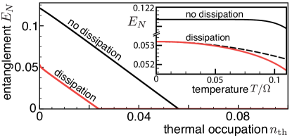
and the variances are given by and where is the thermal occupation number (we set and ). Entanglement is obtained when the product in Eq. (1) becomes smaller than , which requires a coupling rate . In this expression only terms up to first order in have been considered and we have set . For a given coupling rate the logarithmic negativity decreases linearly as a function of the thermal occupation : (black curve in Fig. 2). Thus, as is well known, thermal fluctuations will reduce and eventually destroy entanglement.
III 3. Exact solution
Returning to the full model, an exact description of the dissipative dynamics is provided by quantum Langevin equations 2000_GardinerZoller_QuNoise for the Heisenberg operators, obtained by eliminating the bath degrees of freedom:
| (2) |
where and . denotes stationary quantum noise forces acting on the oscillators (with ). The response functions that take into account the memory effect of the baths are given by . Solving Eq. (2) in Fourier space yields position correlators . Here and are elements of a matrix whose inverse is given by and for . Momentum correlators follow from , and . Finally, equal-time correlators are obtained by integration, . The solution of Eq. (2) thus provides the full covariance matrix in terms of frequency integrals over arbitrary bath spectra, and from it the logarithmic negativity for two coupled dissipative oscillators. Note that we did not assume equilibrium, i.e., the fluctuation-dissipation relation between and does not necessarily hold.
For simplicity, we will from now on restrict our explicit calculations to the symmetric case of two identical oscillators that couple equally strongly to independent baths, such that and The system can then, as before, be decomposed into the center of mass mode (, ) and the relative mode (, ), which become independent dissipative oscillators. We find , where . After frequency integration, Eq. (1) thus directly yields the logarithmic negativity.
IV 4. Equilibrium bath
First, we illustrate the general scheme for the case of equilibrium baths, picking the important example of an Ohmic bath spectrum: . Here denotes the temperature, the damping rate, and the cutoff frequency. For and , the position and momentum variances of an oscillator coupled to this bath are given analytically in 1992_Weiss_QuDissipativeSystems . Here we only display the expansion to first order in at :
| (3) |
As illustrated in Fig. 2, entanglement between the oscillators is suppressed due to their coupling to the bath. The high-frequency bath modes cause momentum fluctuations that depend logarithmically on the cutoff frequency, cf. Eq. (3). Thus, even at zero temperature, the coupling to the environment reduces the logarithmic negativity by [as follows from Eqs. (1) and (3)], and eventually destroys the entanglement completely. Entanglement persists () only if the coupling rate exceeds a threshold value of
| (4) |
As a distinctive feature, the minimal coupling rate depends logarithmically on the cutoff frequency. It indicates that any approach that disregards the influence of high-frequency fluctuations has to fail, as discussed for the example of the Lindblad approach below. Our general formula also allows to obtain the full temperature-dependence, cf. Fig. 2.
V 5. Non-equilibrium bath
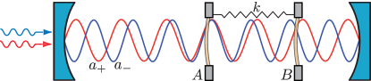
Tunable non-equilibrium quantum fluctuations are now relevant in many contexts, and may be used, e.g., to cool systems below the bulk temperature. A paradigmatic example is the photon shot noise coupled to mechanical resonators in optomechanical setups Examples_Optomechanics ; 2009_FM_ReviewOptomechanics (the following results also apply to analogous electromechanical systems Examples_Microwave ; 2006_Naik_CoolingNanomechResonator ). We treat the conceptually clearest case where two nanomechanical membranes are placed inside a laser-driven cavity and two independent light forces act on the mechanical normal modes leading to optomechanical cooling 2007_FM_SidebandCooling ; 2007_Wilson-Rae_TheoryGroundStateCooling . This may be realized in a setup with two cavity modes, where , cf. Fig. 3. Here are the annihilation operators of the cavity modes, is the mechanical ground-state width, and is the oscillator-cavity coupling rate that scales linearly with the laser amplitude (see 2009_Hammerer_StrongCoupling ; 2010_Wallquist_PRA for a derivation of this type of coupling). The mechanical coupling between the oscillators (here assumed as given) can itself be implemented via other, strongly driven far-detuned cavity modes 2008_Hartmann ; 2009_Hammerer_StrongCoupling . Other possible setups include cold-atom or hybrid atom-membrane systems 2009_Hammerer_StrongCoupling .
Elimination of the cavity degrees of freedom generates cavity noise spectra 2007_FM_SidebandCooling , where is the decay rate of the cavity photons and the detuning of the corresponding input lasers with respect to the first (second) cavity mode. A spectrum of this kind induces an optomechanical cooling rate of . In the optimal cooling regime, for and , we have . In this regime, the minimum possible phonon number due to optical cooling, defined by , will be much smaller than 1 (). Moreover, we assume and as required for ground state cooling. The full forces also contain thermal fluctuations, , independent from . For low mechanical damping () the spectrum of the thermal bath can be replaced by the values at the resonances, i.e., . The general scheme yields the variances by integrating and .
In the optimal cooling regime, the variances of the optomechanically damped system can be expressed in a compact way:
| (5) | |||||
| (6) |
where and .
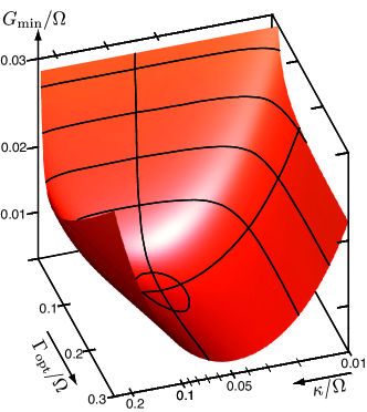
Together with Eq. (1), these formulas constitute our main result for entanglement in a system subject to optomechanical cooling. We now extract and discuss its main physical features. The first term on the rhs. of Eq. (5) describes the ground state energy, and the second term takes account of the cooling mechanism: the thermal occupation is reduced to an effective phonon number . Thus, entanglement can in principle be created even for large bulk temperatures, , if the optomechanical damping rate is sufficiently large. Since , this can be achieved either by reducing the cavity linewidth or by increasing the cavity-oscillator coupling rate . However, we identify two processes that destroy entanglement for small and large , respectively. First, as known from 2007_FM_SidebandCooling , the cooling mechanism becomes less efficient in the strong coupling regime , where the contribution of becomes appreciable. Second, for a large optomechanical coupling strength , the low-frequency contributions of the photon shot noise induce an increase of the position variance [second term on the rhs. of Eq. (6)]. This implies that strong correlations between the individual oscillators and the driven cavity lead to a destruction of entanglement between the oscillators.
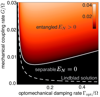
As a consequence, entanglement depends non-monotonically on the cavity linewidth and the optomechanical damping rate in the optimal cooling regime, cf. Figs. 4 and 5. Entanglement can be generated only if the mechanical coupling rate exceeds a value of
| (7) |
Note that Eq. (7) can be employed to optimize entanglement.
VI 6. Shortcomings of the Lindblad approach
The crucial destruction of entanglement by strong dissipation is missed entirely by the commonly employed Lindblad master equation approach. Its general form is given by , where the influence of the bath is taken into account by Lindblad terms 2000_GardinerZoller_QuNoise . For equilibrium baths, these are given by and where and are the mechanical normal mode annihilation operators. At zero temperature, the shortcomings of the Lindblad approach are most obvious: The system evolves into its ground state, whose entanglement is not reduced at all by the system-bath coupling. To treat the non-equilibrium case of Fig. 3 in the Lindblad approach, we have to consider four additional terms, and , which take account of the decoherence via the cavity modes (see 2010_Wallquist_PRA for a detailed derivation). The steady-state variances of the normal modes follow as This expression describes the cooling to an effective phonon number but fails to capture the loss of entanglement for strong optomechanical coupling (see the dashed curve in Fig. 4). The shortcomings of this approach can be understood by noting that the Born-Markov approximation, which assumes the bath to have a very short correlation time (no memory) and to be uncorrelated with respect to the system, does not hold in general for a non-equilibrium bath as can be seen in our example.
VII 7. Conclusions and outlook
The general exact framework introduced here can be employed to analyze the entanglement of oscillators under the influence of arbitrary bath spectra, among them non-equilibrium and tailored non-standard spectral densities. As pointed out in this paper, the effects of tunable non-equilibrium environments promise rich physics to be explored in current experimental setups. The optomechanical setup investigated here is in fact just one of a rather large class of setups to which this work applies, and which also extends into the fields of electromechanics Examples_Microwave ; 2006_Naik_CoolingNanomechResonator and cold-atom physics 2009_Hammerer_StrongCoupling . We also note that completely different systems show similar entanglement production effects under non-equilibrium conditions, as has been explored in the case of coupled, driven qubits 2009_Li_EntanglementInDrivenQubitSystems , atoms EntanglementProduction_Atoms and ions 2002_Schneider_EntanglementInDickeModel , or coupled double quantum dots 2007_Lambert_NoneqEntanglement .
In the quest to observe entanglement in dissipatively cooled optomechanical or nanoelectromechanical systems the theory presented here serves as an essential guideline: It identifies viable parameter regimes for generating and optimizing entanglement between massive mechanical oscillators.
Recent works Entanglement_ParametricAmplification ; 2010_Wallquist_PRA have proposed an alternative way of generating entanglement in nanomechanical systems: By modulation the coupling strength between the oscillators the system can be parametrically driven into a non-equilibrium state which features entanglement even at relatively large temperatures. In a future work the general framework introduced here can be employed to discuss the generation of entanglement in a parametrically driven system and to compare and connect the two approaches.
VIII Acknowledgments
Support by the DFG through NIM, SFB631 and the Emmy-Noether program, by the Austrian Science Fund through SFB FOQUS, and by the IQOQI is acknowledged.
References
- [1] E. Schrödinger. Naturwissenschaften 23, 823 (1935).
- [2] R. Horodecki, P. Horodecki, M. Horodecki and K. Horodecki, Rev. Mod. Phys. 81, 865 (2009).
- [3] W. Dür and H.-J. Briegel, Phys. Rev. Lett. 92, 180403 (2004); J. Eisert, M. B. Plenio, S. Bose and J. Hartley, textitibid. 93, 190402 (2004); J. P. Paz and A. J. Roncaglia, /textitibid. 100, 220401 (2008); T. Yu and J. H. Eberly, Science 323, 598 (2009).
- [4] for recent experiments, see: J. D. Thompson, B. M. Zwickl, A. M. Jayich, F. Marquardt, S. M. Girvin and J. G. E. Harris, Nature 452, 900 (2008); S. Groblacher, J. B. Hertzberg, M. R. Vanner, G. D. Cole, S. Gigan, K. C. Schwab and M. Aspelmeyer, Nat. Phys. 5, 485 (2009); A. Schliesser, O. Arcizet, R. Riviere, G. Anetsberger and T. J. Kippenberg,ibid. 5, 509 (2009).
- [5] J. D. Teufel, J. W. Harlow, C. A. Regal and K. W. Lehnert, Phys. Rev. Lett. 101, 197203 (2008); T. Rocheleau, T. Ndukum, C. Macklin, J. B. Hertzberg, A. A. Clerk and K. C. Schwab, Nature 463, 72 (2010).
- [6] A. Naik, O. Buu, M. D. LaHaye, A. D. Armour, A. A. Clerk, M. P. Blencowe, and K. C. Schwab, Nature 443, 193 (2006).
- [7] K. C. Schwab and M. L. Roukes, Phys. Today58 (7), 36 (2005).
- [8] M. Pinard, A. Dantan, D. Vitali, O. Arcizet, T. Briant and A. Heidmann, Europhys. Lett. 72, 747 (2005); D. Vitali, S. Mancini and P. Tombesi, J. Phys. A. 40, 8055 (2007); C. Wipf, T. Corbitt, Y. Chen, N. Mavalvala, New J. Phys. 10, 095017 (2008); H. Muller-Ebhardt, H. Rehbein, R. Schnabel, K. Danzmann, Y. Chen, Phys. Rev. Lett. 100, 013601 (2008).
- [9] M. J. Hartmann and M. B. Plenio, Phys. Rev. Lett. 101, 200503 (2008).
- [10] J. Eisert and M. B. Plenio, J. Mod. Opt 46, 145 (1999).
- [11] R. Simon, Phys. Rev. Lett. 84, 2726 (2000).
- [12] G. Vidal and R. F. Werner, Phys. Rev. A 65, 032314 (2002).
- [13] C. W. Gardiner and P. Zoller, Quantum Noise, 3rd ed. (Springer, Berlin, 2004).
- [14] U. Weiss, Quantum Dissipative Systems (World Scientific, Singapore, 1993)
- [15] For a review, see F. Marquardt and S. M. Girvin, Physics 2, 40 (2009).
- [16] F. Marquardt, J. P. Chen, A. A. Clerk, and S. M. Girvin, Phys. Rev. Lett. 99, 093902 (2007).
- [17] I. Wilson-Rae, N. Nooshi, W. Zwerger, and T. J. Kippenberg, Phys. Rev. Lett. 99, 093901 (2007).
- [18] K. Hammerer, M. Wallquist, C. Genes, M. Ludwig, F. Marquardt, P. Treutlein, P. Zoller, J. Ye, and H. J. Kimble, Phys. Rev. Lett. 103, 063005 (2009).
- [19] M. Wallquist, K. Hammerer, P. Zoller, C. Genes, M. Ludwig, F. Marquardt, P. Treutlein, J. Ye, and H. J. Kimble, Phys. Rev. A 81, 023816 (2010).
- [20] J. Li and G. S. Paraoanu, New J. Phys. 11, 113020 (2009).
- [21] S. Mancini and S. Bose, Phys. Rev. A 64, 032308 (2001); X. X. Yi, C. S. Yu, L. Zhou, and H. S. Song, ibid. 68, 052304 (2003); S. Mancini and J. Wang, Eur. Phys. J. D 32, 257 (2005); J. Wang, H. M. Wiseman, and G. J. Milburn, Phys. Rev. A 71, 042309 (2005).
- [22] S. Schneider and G. J. Milburn, Phys. Rev. A 65, 042107 (2002).
- [23] N. Lambert, R. Aguado, and T. Brandes, Phys. Rev. B 75, 045340 (2007).
- [24] L. Tian, M.S. Allman and R. W. Simmonds, New J. Phys. 10, 115001 (2008), F. Galve and E. Lutz, Phys. Rev. A 79, 032327 (2009), A. Mari and J. Eisert, Phys. Rev. Lett. 103, 213603 (2009), F. Galve, L. A. Pachon and D. Zueco, arXiv:1002.1923 (2010).