Spectral properties of a resonator driven by a superconducting single-electron transistor

Abstract

We analyze the spectral properties of a resonator coupled to a superconducting single electron transistor (SSET) close to the Josephson quasiparticle resonance. Focussing on the regime where the resonator is driven into a limit-cycle state by the SSET, we investigate the behavior of the resonator linewidth and the energy relaxation rate which control the widths of the main features in the resonator spectra. We find that the linewidth becomes very narrow in the limit-cycle regime, where it is dominated by a slow phase diffusion process, as in a laser. The overall phase diffusion rate is determined by a combination of direct phase diffusion and the effect of amplitude fluctuations which affect the phase because the resonator frequency is amplitude dependent. For sufficiently strong couplings we find that a regime emerges where the phase diffusion is no longer minimized when the average resonator energy is maximized. Finally we show that the current noise of the SSET provides a way of measuring both the linewidth and energy relaxation rate.

I Introduction

When a resonator is coupled to a superconducting single-electron transistor (SSET) tuned close to the Josephson quasiparticle (JQP) resonance the flow of charges can either damp the resonator motion, potentially leading to cooling,clerk:05 ; blencowe:05 or pump itbennett:06 ; rodrigues:07a ; marthaler:08 ; harvey:08 ; andre:09 ; ashhab:09 leading to laser-like states of self-sustaining oscillation, depending on the choice of operating point. Recent experiments using a superconducting stripline resonator coupled capacitively to the SSET island demonstrated a laser effect astafiev:07 whilst the opposite effect of cooling was demonstrated using a nanomechanical resonator. naik:06 Similar cooling effects and laser like instabilities occur close to other transport resonances in the SSET-resonator system,clerk:05 ; bennett:06 ; koerting:09 as well as in apparently rather different systems such as a driven optical cavity coupled parametrically to a mechanical resonator.kippenberg:08 ; favero:09 ; marquardt:09 Furthermore, useful analogies can be maderodrigues:07 ; you:07 ; marthaler:08 with quantum optical systems such as the micromaser where a cavity resonator interacts with a sequence of two level atoms.englert:02

The SSET is tuned to the JQP resonance by appropriate choices of the drain source and gate voltages applied nazarov:09 ; aleshkin:90 ; choi:03 (see Fig. 1 for a schematic illustration of the JQP cycle). Close to the resonance the charge dynamics of the SSET island is similar to a driven two-level system coupled to a bath.hauss:08 ; jaehne:08 Charge is transported through the system via a combination of coherent tunneling of a Cooper-pair and two successive quasiparticle decay processes. The center of the resonance occurs when two states of the SSET island differing by a single Cooper-pair, $|0\rangle$ and $|2\rangle$ have the same charging energy. For operating points where the electrostatic energy of state $|2\rangle$ is less than that of the $|0\rangle$ state the SSET tends to emit energy to the resonator.clerk:05 ; blencowe:05 The decay processes in the SSET generate a current whose average value and fluctuations provide a natural source of information about the dynamics of the resonator.harvey:08 ; koerting:09

For sufficiently strong coupling, the energy emitted to the resonator can lead to a variety of different limit-cycle states.clerk:05 ; bennett:06 ; rodrigues:07 The existence of the limit-cycle states is shown clearly in the steady state properties of the resonator’s density matrix. However, information about the important dynamical time-scales of the system such as the resonator linewidth and energy relaxation rate is only obtained by going beyond the steady-state of the system to examine the spectrum of fluctuations that occur about this state.

Figure 1: (a) Superconducting single electron transistor: two tunnel junctions and a gate capacitor $C_{g}$ form the SSET island to which the resonator is coupled capacitively. A drain source voltage, $V_{\rm ds}$, and gate voltage, $V_{\rm g}$, are used to tune the operating point of the device. (b) JQP cycle: Cooper-pair tunneling at the left hand junction between island states $|0\rangle$ and $|2\rangle$ is interrupted by two quasiparticle tunneling events which take the island charge back to $|0\rangle$ via the $|1\rangle$ state.

In this paper we use a combination of numerical and analytical methods to investigate the spectral properties of a resonator pumped by a SSET tuned close to the JQP resonance. Direct numerical evaluation of the relevant spectra allows us to obtain both the energy relaxation rate and linewidth of the resonator. We find that except within transition regions, the peaks in the resonator spectra have a Lorentzian shape with widths that correspond to the real parts of particular individual eigenvalues of the system. For weak to moderate couplings the resonator linewidth behaves in a way that is typical of self-sustained oscillators:lax:67 below threshold it is simply half the energy relaxation rate of the resonator, while above threshold, in the limit-cycle regime, it becomes much narrower. We show that the linewidth in the limit-cycle regime is set by the phase diffusion rate of the system in a way that is similar to a laser.walls:94 For sufficiently strong coupling we find that a more complex behavior emerges and the operating points (of the SSET) at which the linewidth is narrowest no longer correspond to the point where the resonator energy is maximized, an effect which was also seen in a recent study of a very similar system.andre:09 We further show that the full current noise spectrum of the SSET gives direct access to the energy relaxation ratekoerting:09 and, within a limit-cycle state, the phase diffusion rate of the resonator.

This work is organized as follows. Sec. II is devoted to the simple model we use to describe the SSET-resonator system and the methods used in its solution. We begin by outlining the Born-Markov master equation for the system, in which the evolution of the reduced density matrix is given by a Liouvillian superoperator, and then summarize the steady state properties of the resonator. Next we describe the method used to calculate the resonator spectra numerically. In Sec. III we give the numerically calculated fluctuation spectra of the resonator. Following a characterization of the features observed we go on to show how the eigenvalues of the Liouvillian matrix can be used to obtain the widths of the peaks observed in the spectra. The calculation of the eigenvalues is significantly less challenging numerically than a full calculation of the spectra, allowing us to then investigate the behavior of the linewidth for a range of coupling strengths. To understand the observed behavior of the linewidth we make use of an analytical approximation in Sec. IV and thereby link the eigenvalues to the relevant physical processes in the system. Finally, in Sec. V we show that the current noise spectrum of the system can be used to measure the linewidth and energy relaxation rate of the resonator. The Appendix contains additional details of the analytical calculations.

II Model

II.1 Master Equation

The Born-Markov master equation describing the evolution of the reduced density matrix, $\rho(t)$, of the SSET and resonator in the vicinity of the JQP resonance is given by,rodrigues:07 ; rodrigues:07a

$$\dot{\rho}(t) =-\frac{i}{\hbar}\left[H_{\rm co},\rho(t)\right]+\mathcal{L}_{\rm qp}\rho(t)+\mathcal{L}_{\rm d}\rho(t)$$

$$=\mathcal{L}\rho(t).$$ (1)

The first term describes the coherent evolution of the density matrix under the Hamiltonian $H_{\rm co}$,

$$H_{\rm co} = \Delta E|2\rangle\langle 2|-\frac{E_{J}}{2}\left(|0\rangle\langle 2|+|2\rangle\langle 0|\right)+\frac{p^{2}}{2m}$$ (2)

$$+\frac{1}{2}m\Omega^{2}x^{2}+m\Omega^{2}x_{s}x\left(|1\rangle\langle 1|+2|2\rangle\langle 2|\right),$$

where $\Delta E$ is the detuning from the JQP resonance and $E_{J}$ is the Josephson coupling energy. The resonator has frequency $\Omega$, effective mass $m$, momentum operator $p$, position operator $x$ and $x_{s}$ parameterizes the SSET-resonator coupling strength. The second and third terms of Eq. 1 describe the dissipative effects of quasiparticle tunneling and the resonator’s environment respectively,

$$\mathcal{L}_{\rm qp}\rho(t) =\Gamma|0\rangle\langle 1|\rho(t)|1\rangle\langle 0|+\Gamma|1\rangle\langle 2|\rho(t)|2\rangle\langle 1|$$

$$-\frac{\Gamma}{2}\left\{|1\rangle\langle 1|+|2\rangle\langle 2|,\rho(t)\right\},$$ (3)

$$\mathcal{L}_{\rm d}\rho(t) =-\frac{\gamma_{\rm ext}m\Omega}{\hbar}\left(n_{\rm ext}+\frac{1}{2}\right)\left[x,\left[x,\rho(t)\right]\right]$$

$$-\frac{i\gamma_{\rm ext}}{2\hbar}\left[x,\left\{p,\rho(t)\right\}\right],$$ (4)

where $\Gamma$ is the quasiparticle tunneling rate and $\{\cdot\,,\cdot\}$ is the anti-commutator. The effects of the resonator’s environment are parameterized by the external damping rate $\gamma_{\rm ext}$ and the thermal occupation number $n_{\rm ext}=({\rm e}^{\hbar\Omega/k_{\rm B}T_{\rm ext}}-1)^{-1}$, with $T_{\rm ext}$ the temperature. We have neglected the (weak) dependence of $\Gamma$ on the position of the resonator and the difference in the tunneling rates of the two quasiparticle decay processes.rodrigues:07

For the numerical analysis of the system we use a Liouville space representation,blum:96 ; briegel:93 ; jacob:04 ; flindt:04a ; brandes:08 following the notation introduced in Ref. harvey:08, . The Liouvillian,djuric:06 ; harvey:08 $\mathcal{L}$, appearing in Eq. 1, can be expressed in terms of an eigenvector expansion,

$$\mathcal{L}=\sum_{p=0}^{\infty}\lambda_{p}|l_{p}\rangle\!\rangle\!\langle\!\langle r_{p}|,$$ (5)

where $|r_{p}\rangle\!\rangle$ are the right hand eigenvectors, $\langle\!\langle l_{p}|$ the left hand eigenvectors and $\lambda_{p}$ the associated eigenvalues. The steady-state density matrix in Hilbert space $\rho_{\rm ss}$ is equivalent to the right hand eigenvector in Liouville space corresponding to the eigenvalue $\lambda_{0}=0$, i.e. $\rho_{\rm ss}\Leftrightarrow|r_{0}\rangle\!\rangle$. Multiplication on the left by $\langle\!\langle l_{0}|$ is the equivalent of the Hilbert space trace operation,flindt:04a $\langle\!\langle l_{0}|\rho(t)\rangle\!\rangle={\rm Tr}[\rho(t)]$.

An appropriate truncation of the oscillator basis allows Eq. (1) to be solved numerically to find the relevant eigenvalues and eigenvectors of $\mathcal{L}$. We do this by using the Matlab implementation of the ARPACK linear solver.lehoucq:98 In order to use a large number of resonator states we neglect the parts of the density matrix corresponding to coherences involving the $|1\rangle$ state since these are decoupled from the charge states of the system.rodrigues:07 Additionally we make the approximation that the coherence between resonator energy levels with a large separation in energy can be neglected.harvey:08 ; koerting:09

II.2 Steady state behavior

We now briefly review the steady-state properties of the resonator as a function of the dimensionless coupling strength $\kappa=\frac{m\Omega^{2}x_{s}^{2}}{eV_{\rm ds}}$ and the detuning $\Delta E$ as this will provide important points of reference for the study of the spectral properties in the following sections. For concreteness we focus our analysis on the regime of a high frequency resonator in comparison to the relaxation time of the SSET ($\Omega\gg\Gamma$), which is achievable in experiments using a superconducting stripline resonator.astafiev:07 This complements previous work on the low frequency regime,clerk:05 ; bennett:06 although we note that our methods are also suitable for a slow resonator. For this kind of resonator the temperature can be sufficiently low for thermal effects to be unimportant and so we take $n_{\rm ext}=0$ throughout. We also choose to work in a regime where the Josephson coupling is relatively weak compared to the quasiparticle decay rate and hence we take $\Gamma=V_{\rm ds}/eR_{J}$. We use a value for the Josephson energy of $E_{J}=1/16\,eV_{\rm ds}$, with a junction resistance $R_{J}=h/e^{2}$. Working in this regime has the advantage that it is also possible to develop an approximate analytical description of the dynamics.rodrigues:07 ; rodrigues:08 Furthermore, when the quasiparticle decay rate is relatively large this should be the dominant source of dephasing for the SSET island charge and so we do not need to consider additional environmental effects.

When $\Omega\gg\Gamma$ the interaction between the SSET and resonator is quite weak except for near values of $\Delta E$ where there is a matching of the eigenenergy of the SSET to the energy level separation in the resonator,

$$k\hbar\Omega=\pm\sqrt{\Delta E^{2}+E_{J}^{2}},$$ (6)

where $k$ is a non-zero integer and the sign should match the sign of $\Delta E$. For $\Delta E<0$ ($k<0$) these resonances correspond to the transfer of energy from the SSET to the resonator. For sufficient coupling the resonator is driven into states of self-sustained oscillations.rodrigues:07a

The steady state of the resonator is nicely described by the distribution $P(n)={\rm Tr}[|n\rangle\langle n|\rho_{\rm ss}]$, where $|n\rangle$ is a Fock state of the resonator. The resonator is said to be in a fixed point state when the $P(n)$ distribution has a single peak at $n=0$. We define a well-defined limit-cycle state as corresponding to a $P(n)$ distribution with a peak at $n\neq 0$ and additionally a small value for $P(0)$ (for the purposes of plotting we choose ‘small’ to mean $P(0)\leq 1\times 10^{-5}$). Finally we define the transition region between the two states. In the regimes studied here this occurs via a continuous transition, starting from a fixed point state increasing the coupling $\kappa$ leads first to a wider $P(n)$ distribution and then the peak in the distribution moves away from $n=0$. We define the transition region as when the peak in $P(n)$ is at $n\neq 0$ but there is also substantial weight at $P(0)$ (again we choose $P(0)>1\times 10^{-5}$). Although this particular definition of the transition region is of course somewhat arbitrary, it nevertheless proves a useful indicator in what follows. The resonator can display bistable (and multistable) behavior in this system,rodrigues:07a but here we focus only on a parameter range where this is not the case and the $P(n)$ distribution only ever has a single peak.

The steady state properties of the resonator, $\left\langle n\right\rangle=\left\langle a^{\dagger}a\right\rangle$, where $a$ is the resonator lowering operator, and $F_{n}=\left\langle\bar{n}^{2}\right\rangle/\left\langle n\right\rangle$, with $\bar{n}=n-\left\langle n\right\rangle$, are shown in Figs. 2a and 2b for varying detunings and coupling strengths. The plots are centered around the $k=-1$ resonance [Eq. (6)], which for our parameters occurs at $\Delta E=-1.59\,eV_{\rm ds}$. Similar plots were given in Ref. harvey:08, , but here we go to higher coupling. As the coupling is increased we see that $\left\langle n\right\rangle$ increases on resonance up to a maximum value for $\kappa\simeq 0.005$ and then decreases. $F_{n}$ shows a large peak at the point where the peak in the $P(n)$ distribution moves from $n=0$ to $n\neq 0$ [see Fig. 2b harvey:08 ]. The value of $F_{n}$ drops as the coupling is increased further and the system develops a well-defined limit-cycle state. The value of $F_{n}$ drops below unity (i.e. becomes sub-Poissonian) for sufficiently strong coupling ($\kappa\gtrsim 0.0075$ in Fig. 2b).

Figure 2: (Color online) (a) Average resonator energy $\left\langle n\right\rangle$ and (b) Fano factor $F_{n}$, for varying $\Delta E$ and $\kappa$, with $\Omega=10$ and $\gamma_{\rm ext}=3\times 10^{-4}$ (we adopt units such that $\Gamma=1$). Within the inner dashed line the resonator is in a limit-cycle state, between the two lines it is in the transition region (as defined in the text) and elsewhere it is in a fixed point state.

II.3 Noise spectra of the system

The steady-state of a system only gives information about average quantities. By also calculating noise spectra, further important information about the dynamics of the system can be obtained. We define the symmetrized noise spectrum for the two operators $b$ and $b^{\dagger}$ as,

$$S_{b,b^{\dagger}}(\omega) = \lim_{t\to\infty}\int_{-\infty}^{\infty}d\tau\left\langle\{\bar{b}(t+\tau),\bar{b}^{\dagger}(t)\}\right\rangle e^{i\omega\tau}$$ (7)

$$= 2\Re\lim_{t\to\infty}\int_{0}^{\infty}d\tau\left\langle\{\bar{b}(t+\tau),\bar{b^{\dagger}}(t)\}\right\rangle e^{i\omega\tau},$$ (8)

where $\bar{b}(t)=b(t)-\left\langle b\right\rangle$, $\left\langle b\right\rangle={\rm Tr}[b\rho_{\rm ss}]$ and $\Re$ indicates the real part. The symmetrized noise spectrum has the property $S_{b,b^{\dagger}}(\omega)=S_{b^{\dagger},b}(-\omega)$. Note that we consider fluctuations about the steady-state of the system represented by the limit $t\to\infty$.

For system operators the correlation function can be evaluated by using the quantum regression theorem (QRT). The QRT states that the two-time correlation function can be written,walls:94

$$\lim_{t\to\infty}\left\langle b(t+\tau)b^{\dagger}(t)\right\rangle=\text{Tr}\!\left[be^{\mathcal{L}\tau}b^{\dagger}\rho_{\rm ss}\right],\qquad\tau\geq 0.$$ (9)

In Liouville space this leads to,flindt:04a

$$S_{b,b^{\dagger}}(\omega)=4\Re\langle\!\langle l_{0}|\mathcal{B}\mathcal{R}(\omega)\mathcal{B}^{\dagger}|r_{0}\rangle\!\rangle,$$ (10)

where $\mathcal{B}$ is the Liouville space symmetrized superoperator whose relation to the Hilbert space operator $b$ is given by,

$$\mathcal{B}|\rho(t)\rangle\!\rangle\Leftrightarrow\frac{1}{2}\left(b\rho(t)+\rho(t)b\right),$$ (11)

and we define the pseudo-inverse of the Liouvillian,

$$\mathcal{R}(\omega)=\mathcal{W}\left(-i\omega-\mathcal{L}\right)^{-1}\mathcal{W},$$ (12)

with $\mathcal{W}$ an operator that projects away from the steady-state of the system, $\mathcal{W}\equiv 1-|r_{0}\rangle\!\rangle\!\langle\!\langle l_{0}|$. The matrix formulation, given in Eq. (10), is used to numerically evaluate the noise spectra in the next section.

We can obtain helpful approximations and considerable insight into how the resonator dynamics affect the noise by performing an eigenfunction expansion of the Liouvillian [Eq. (5)] in $\mathcal{R}(\omega)$ to obtain the alternative form for the spectrum,

$$S_{b,b^{\dagger}}(\omega) =4\Re\left[\sum_{p=1}^{\infty}\frac{1}{-i\omega-\lambda_{p}}\langle\!\langle l_{0}|\mathcal{B}|r_{p}\rangle\!\rangle\!\langle\!\langle l_{p}|\mathcal{B}^{\dagger}|r_{0}\rangle\!\rangle\right]$$

$$=-4\sum_{p=1}^{\infty}\frac{\Re[\lambda_{p}]\Re[m_{B}^{p}]-(\Im[\lambda_{p}]+\omega)\Im[m_{B}^{p}]}{\Re[\lambda_{p}]^{2}+(\Im[\lambda_{p}]+\omega)^{2}},$$ (13)

where $m_{B}^{p}=\langle\!\langle l_{0}|\mathcal{B}|r_{p}\rangle\!\rangle\!\langle\!\langle l_{p}|\mathcal{B}^{\dagger}|r_{0}\rangle\!\rangle$. In almost all the cases considered here $m_{B}^{p}$ turns out to be real, and each term in the sum corresponds to a Lorentzian. However, in the case of the current noise we find that $\Im[m_{B}^{p}]\neq 0$, leading to a somewhat more complex lineshape,rodrigues:08 a point which we discuss further in Sec. V.

A knowledge of the eigenvalues of the system tells us where we can expect features in the spectra and how wide these features are. For the two separate systems of a damped oscillator and the SSET near the JQP resonance the eigenvalues are easily obtained. The eigenvalues for an oscillator coupled to a thermal bath are,englert:02

$$\lambda=-im\Omega-\left(l+\frac{1}{2}|m|\right)\gamma_{\rm ext}\quad\begin{array}[]{l}l=0,1,2,\ldots\\ m=0,\pm 1,\pm 2,\ldots\end{array}$$ (14)

The eigenvalues of the SSET do not have such a simple analytic form. For small $E_{J}$, the non-zero eigenvalues consist of a conjugate pair with a real part $\sim-\Gamma/2$ and imaginary parts close to the SSET frequency $\Omega_{\rm SSET}=\sqrt{\Delta E^{2}+E_{J}^{2}}/\hbar$, with the others real and of order $-\Gamma$. In the limit of zero coupling, the eigenvalues of the combined system will just be the sum and difference of these eigenvalues.

III Spectral properties of the resonator

The first resonator spectrum we consider is

$$S_{a,a^{\dagger}}(\omega) =\lim_{t\to\infty}\int_{-\infty}^{\infty}d\tau\left\langle\{\bar{a}(t+\tau),\bar{a^{\dagger}}(t)\}\right\rangle e^{i\omega\tau}$$

$$=4\Re\langle\!\langle l_{0}|\mathcal{A}\mathcal{R}(\omega)\mathcal{A}^{\dagger}|r_{0}\rangle\!\rangle,$$ (15)

where $\mathcal{A}|\rho(t)\rangle\!\rangle\Leftrightarrow\frac{1}{2}\left(a\rho(t)+\rho(t)a\right)$. The width of the peak that appears at the resonator frequency in this spectrum is the resonator linewidth, $\gamma_{\Omega}$. For a superconducting stripline resonator this spectrum can be inferred by probing the field that leaks out of the resonator walls:94 (e.g. via capacitive coupling to a transmission line astafiev:07 ), but here we will focus instead [in Sec. V] on how the current noise spectrum can be used to obtain the resonator linewidth. For a resonator coupled only to a thermal bath this spectrum consists of a single Lorentzian peak at the frequency of the resonator, with a width given by half the energy relaxation rate which in this case is simply $\gamma_{\rm ext}/2$.

The behavior of $S_{a,a^{\dagger}}(\omega)$ for $\Delta E$ detuned away from the center of the $k=-1$ resonance [Eq. (6)] (where the resonator is in a fixed point state) and at the resonance (with $\kappa$ such that the system is just inside the region where a well-defined limit-cycle exists) is shown in Figs. 3a and 3b respectively. For the off-resonant case, peaks are observed at $\omega=0$, $\omega\simeq\Omega$, $\omega\simeq\Omega_{\rm SSET}$, $\omega\simeq\Omega-\Omega_{\rm SSET}$ and $\omega\simeq-\Omega+\Omega_{\rm SSET}$. When at resonance we also observe the appearance of additional peaks at higher multiples of the resonator frequency. Also note that the peaks involving the SSET frequency have a much larger width since $\Gamma\gg\gamma_{\rm ext}$.

Figure 3: (Color online) Resonator spectrum $S_{a,a^{\dagger}}(\omega)$ for $\kappa=0.003$ (other parameters are the same as in Fig. 2). (a) off-resonance $\Delta E=-1.75\,eV_{\rm ds}$, $\Omega_{\rm SSET}=1.1\Omega$ on a $\log_{10}$ scale, (b) on-resonance $\Delta E=-1.59\,eV_{\rm ds}$, $\Omega_{\rm SSET}=\Omega$ on a $\log_{10}$ scale. The insets show the behavior around the peak at $\omega\simeq\Omega$ without logarithmic scaling (full lines) along with Lorentzian fits to the peaks (dashed lines).

The spectra are dominated by the peak near to the frequency of the resonator, which is shown in detail in the insets. In each case the position of the peak is shifted slightly from the bare frequency of the resonator due to a renormalization arising from the interaction with the SSET. In both cases the peak remains Lorentzian. By comparing these two plots alone we see that the linewidth is much narrower for the resonant case. The spectra are shown for a relatively small value of $\kappa$, but for increased coupling similar features are observed.

We also calculate the spectrum of energy fluctuations in the resonator,

$$S_{n,n}(\omega) =\lim_{t\to\infty}\int_{-\infty}^{\infty}d\tau\left\langle\{\bar{n}(t+\tau),\bar{n}(t)\}\right\rangle e^{i\omega\tau}$$

$$=4\Re\langle\!\langle l_{0}|\mathcal{N}\mathcal{R}(\omega)\mathcal{N}|r_{0}\rangle\!\rangle.$$ (16)

where $\mathcal{N}|\rho(t)\rangle\!\rangle\Leftrightarrow\frac{1}{2}\left(n\rho(t)+\rho(t)n\right)$. For a resonator alone this spectrum consists of a single peak at $\omega=0$ with a width, $\gamma_{n}$, given by the energy relaxation rate ($\gamma_{\rm ext}$ in this case) and height $4\left\langle\bar{n}^{2}\right\rangle/\gamma_{\rm ext}$. For the coupled system the peak at $\omega=0$ is found to be Lorentzian to a very good approximation in both the limit-cycle and fixed point regimes, but not within the transition region. We show in Sec. IV that the width of this peak, $\gamma_{n}$, is still given by the energy relaxation rate of the resonator in both the limit-cycle and fixed point states.

The behavior of the resonator linewidth, $\gamma_{\Omega}$, and the rate $\gamma_{n}$ obtained from Lorentzian fits to the appropriate spectral peaks are shown as a function of $\Delta E$ in Fig. 4. The behavior far from resonance is well-understood: the resonator remains in the fixed point state and the SSET acts on it like an effective thermal bathclerk:05 ; blencowe:05 ; rodrigues:08a ; harvey:08 leading (for $\Delta E<0$) to a reduction in the energy relaxation rate and an increase in the effective frequency of the resonator. Thus one expects that in this regime the resonator linewidth should be equal to $\gamma_{n}/2$, as we find. Close to the center of the resonance where the resonator is in a well-developed limit-cycle state there is a strong suppression of the linewidth, whilst the energy relaxation rate remains much larger. This behavior is precisely what one expects for a self-sustained oscillator.lax:67

Figure 4: (Color online) Width of zero frequency peak in the $S_{n,n}(\omega)$ spectrum (upper curves) as determined from a Lorentzian fit ($\gamma_{n}/2$, solid line) and from the smallest non-zero eigenvalue ($-\lambda_{1}/2$, dashed line). The lower curves show the linewidth of the resonator as determined from a Lorentzian fit to $S_{a,a^{\dagger}}(\omega)$ ($\gamma_{\Omega}$, solid line) and from the eigenvalue ($-\Re\lambda_{\Omega}$, dashed line). $\kappa=0.003$ with other parameters the same as in Fig. 2. Vertical dashed lines indicate the transition region.

The fact that a given spectrum can be expressed in terms of the eigenfunction expansion of the Liouvillian as a sum of Lorentzians [Eq. 13] suggests that where the spectral peaks are found to be Lorentzian a single term in the expansion should dominate and the peak width be given by a single eigenvalue. Considering first the spectrum of energy fluctuations, $S_{n,n}(\omega)$, we note that since this is the Fourier transform of the correlation function $\left\langle n(t+\tau)n(t)\right\rangle$, we expect the places where $\left\langle\bar{n}^{2}\right\rangle$ and $S_{n,n}(\omega)$ can be captured by a single term in the eigenfunction expansion to be closely related. In the fixed point and limit-cycle states (but not the transition region) the first term in the eigenfunction expansion describes the variance in the resonator energy rather wellharvey:08 $\left\langle\bar{n}^{2}\right\rangle\simeq\langle\!\langle l_{0}|\mathcal{N}|r_{1}\rangle\!\rangle\!\langle\!\langle l_{1}|\mathcal{N}|r_{0}\rangle\!\rangle$, where the corresponding eigenvalue $\lambda_{1}$ is the smallest non-zero one. The single term approximation to the spectrum is,

$$S_{n,n}(\omega) \simeq 4\Re\left[\frac{1}{-i\omega-\lambda_{1}}\langle\!\langle l_{0}|\mathcal{N}|r_{1}\rangle\!\rangle\!\langle\!\langle l_{1}|\mathcal{N}|r_{0}\rangle\!\rangle\right]$$

$$\simeq\frac{4(-\lambda_{1})\left\langle\bar{n}^{2}\right\rangle}{\omega^{2}+\lambda_{1}^{2}}.$$ (17)

The validity of this expression is confirmed in Fig. 4 where we compare the eigenvalue $\lambda_{1}$ and $\gamma_{n}$ and find excellent agreement except within the transition region, where the $\Omega=0$ peak is not well-described by a Lorentzian and further terms in the eigenfunction expansion are required.

For $S_{a,a^{\dagger}}$ it is expected that the eigenvalue closest to $-i\Omega$ is the most important (this is certainly true for the decoupled system). We denote this eigenvalue $\lambda_{\Omega}$. For the eigenfunction expansion of the steady-state quantity $\left\langle\{\bar{a},\bar{a^{\dagger}}\}\right\rangle$ we find that (for fixed point and limit-cycle states and also in the transition region for weak coupling) the term corresponding to the $\lambda_{\Omega}$ eigenvalue dominates, i.e. $\frac{1}{2}+\left\langle n\right\rangle\simeq\langle\!\langle l_{0}|\mathcal{A}|r_{\Omega}\rangle\!\rangle\!\langle\!\langle l_{\Omega}|\mathcal{A}^{\dagger}|r_{0}\rangle\!\rangle$. Thus we expect that the spectrum around $\omega=\Omega$ should be well approximated by,

$$S_{a,a^{\dagger}}(\omega)\simeq\frac{4(-\Re\lambda_{\Omega})\left(\left\langle n\right\rangle+\frac{1}{2}\right)}{(\omega-\Omega_{R})^{2}+[\Re\lambda_{\Omega}]^{2}},$$ (18)

where $\Omega_{R}$ is the renormalized frequency of the resonator, which is given by the imaginary part of the eigenvalue, $\Omega_{R}=-\Im[\lambda_{\Omega}]$. The comparison of $\gamma_{\Omega}$ with $\Re\lambda_{\Omega}$ in Fig. 4 shows convincing agreement.

The calculation of the eigenvalues is much less numerically intensive than the calculation of the full spectrum, allowing us to calculate the linewidth for a large range of parameters. In Fig. 5a we show the value of $\gamma_{\Omega}$, as determined from the $\lambda_{\Omega}$ eigenvalue, for the same range of parameters as Fig. 2. For weak coupling $\gamma_{\Omega}$ decreases with increasing $\left\langle n\right\rangle$ and hence the maximum in $\left\langle n\right\rangle$ corresponds to a minimum in the linewidth. This behavior is analogous to that seen in a laser where the linewidth above threshold is given by the rate of phase diffusion,walls:94 $\gamma_{\phi}^{\rm laser}=\frac{G}{8\left\langle n\right\rangle}$, where $G$ is the gain. However, a more complex behavior is apparent close to resonance for $\kappa>0.005$ where $\left\langle n\right\rangle$ decreases with increasing $\kappa$ (see Fig. 2) and the (single) maximum in $\left\langle n\right\rangle$ now corresponds to a local maximum in $\gamma_{\Omega}$ with minima on either side.

Figure 5: (Color online) Widths of spectral peaks calculated from the eigenvalues as a function of $\kappa$ and $\Delta E$. (a) $\log_{10}\left[\gamma_{\Omega}\right]$, the logarithm of the linewidth of $S_{a,a^{\dagger}}(\omega)$ (b)$\gamma_{n}$, the width of the zero-frequency peak in $S_{n,n}(\omega)$, (other parameters and lines are as in Fig. 2).

The behavior of $\gamma_{\Omega}$ manifests itself in the height of peak at $\omega\sim\Omega$ in $S_{a,a^{\dagger}}(\omega)$, which from Eq. (18), is $\simeq 4\left\langle n\right\rangle/\gamma_{\Omega}$ ($\left\langle n\right\rangle\gg 1$ in the limit-cycle). The height of this peak as a function of $\Delta E$ initially shows a single maximum at $\Delta E=-1.59\,eV_{\rm ds}$, which splits into a pair of maximas (with a minimum between) as the coupling is increased. Similar behavior was observed in the emission spectrum of a stripline resonator coupled to a SSET in a recent experiment.astafiev:07 However, this experiment was in a rather different parameter regime to the one considered here ($E_{J}\gg\hbar\Gamma$) and in the experiment there were accompanying features in the current, which we do not obtain here. A double peak in the spectral maximum as a function of the detuning from resonance was also predicted in the emission spectrum for a closely related system in Ref. andre:09, . In contrast to the linewidth, the energy relaxation rate $\gamma_{n}$ shown in Fig. 5b shows a similar behavior to that shown in Fig. 4 for all the values of $\kappa$ plotted.

IV Origin of the peak widths

We have shown that the widths of the peaks in the noise spectra are related to the eigenvalues of the Liouvillian, and that when the peaks are Lorentzian, the widths are given by a single eigenvalue corresponding to the dominant noise process. In this section we identify the eigenvalues with physical processes by comparing them to analytic expressions that describe those processes.

We first consider $\gamma_{n}$, the width of the $\omega=0$ peak in $S_{n,n}(\omega)$. We do not expect the correlation function of $n$ to depend on phase, and so in Section III we identified this term as the energy relaxation rate. This is supported by the fact that this term reduces to $\gamma_{\rm ext}$ in the zero-coupling limit. It is well known that when the resonator is in a fixed point state, the energy relaxation rate is given by the sum of the external damping and an additional effective damping due to the SSET,blencowe:05 ; clerk:05 and indeed we find that when the resonator is in a fixed point state, $\gamma_{n}$ is well approximated by this total damping rate. We will now go on to show that $\gamma_{n}$ also corresponds to the energy relaxation rate in the limit-cycle.

In a limit-cycle, the effective damping can be generalized to obtain an amplitude dependent dampingclerk:05 ; bennett:06 ; rodrigues:07 ; rodrigues:08a $\gamma_{\rm eff}(E)$ where $E\approx\left\langle n\right\rangle$ is the average energy. The calculation, which is described in Ref. rodrigues:08a, , proceeds by deriving a set of Langevin equations for the SSET and resonator operators. Assuming then that the resonator energy relaxes much more slowly than the SSET charge, the problem can be separated into two parts (though at the cost of neglecting some of the SSET-resonator correlations). Firstly the SSET charge dynamics can be solved treating the resonator as an harmonic drive with a fixed amplitude. The driven charge response as a function of the resonator amplitude is then used to obtain an effective Langevin equation for the resonator alone.rodrigues:08a Writing down the corresponding equation for the average amplitude of the resonator leads immediately to the effective damping, an expression for which (valid in the limit $E_{J}\ll\Gamma$) is given in the appendix. The average energy of the resonator obeys the equation of motion,

$$\frac{dE}{dt}=-\gamma_{T}(E)E,$$ (19)

where $\gamma_{T}(E)=\gamma_{\rm ext}+\gamma_{\rm eff}(E)$ is the total damping rate. Although this equation is nonlinear, for small fluctuations about a stable limit-cycle with average energy $E_{0}$ (given by $\gamma_{T}(E_{0})=0$) we can linearize this equation to obtain,

$$\frac{dE}{dt} \simeq-\gamma_{\rm lin}\left(E-E_{0}\right)$$

$$\gamma_{\rm lin} =E_{0}\left.\frac{d\gamma(E)_{T}}{dE}\right|_{E=E_{0}},$$ (20)

where $\gamma_{\rm lin}$ is the linearized damping, which gives the energy relaxation rate of the resonator near to a stable limit-cycle solution. The same approach also allows us to calculate the renormalized frequency of the resonator, $\Omega_{R}$ (as we discuss in the appendix).

The calculation of $\gamma_{\rm eff}(E)$ requiresrodrigues:07 ; rodrigues:08a approximations in which certain correlations between the resonator and the SSET are dropped. Not surprisingly, this approach does not capture all of the coupled dynamics of the system and in particular it does not describe the small shift in the SSET frequency which arises due to the coupling to the resonator. This SSET frequency shift is apparent in the plot of $\left\langle n\right\rangle$ in Fig. 2a, where there is a clear change in the position of the peak as the coupling is increased (since this shift is much larger than than $\Omega_{R}-\Omega$, it can be attributed to a shift in $\Omega_{SSET}$). The shifted frequency of the SSET can be obtained from a calculation which includes more of the SSET-resonator correlations (for example from the shift in the SSET eigenvalues within the second order mean field equations described in Ref. harvey:08, ), or simply from the precise location of the peaks in the current noise spectrum of the SSET (Section V). In Fig. 6 we compare $\gamma_{n}$ obtained numerically (from the Liouvillian eigenvalue $\lambda_{1}$) to $\gamma_{\rm lin}$ plotted against $\Delta E$ renormalized to take into account the shift in $\Omega_{SSET}$ (for low-$E_{J}$ and high-$\Omega$, the required renormalization is well approximated by $\Delta\widetilde{E}\approx\Delta E+2\kappa eV_{ds}$). We find good agreement for these parameters which confirms that our identification of $\gamma_{n}$ as the energy relaxation rate is indeed valid. The small difference between the curves in Fig. 6 arises because the expression for $\gamma_{\rm lin}$ is strictly only valid in the small $E_{J}$ limit; we find that a smaller value of $E_{J}$ improves the agreement.

Figure 6: (Color online) Comparison of the width of the zero frequency peak in $S_{n,n}(\omega)$, as given by the eigenvalue $\gamma_{n}(\Delta\tilde{E})$ (solid line), with the energy relaxation rate $\gamma_{\rm lin}(\Delta E)$ (dashed line). Here $\kappa=0.03$, with other parameters the same as in Fig. 2.

We now consider $\gamma_{\Omega}$, the width of the $\omega=\Omega$ peak in $S_{a,a^{\dagger}}(\omega)$. In the fixed point regime, we find that $\gamma_{\Omega}\approx\gamma_{n}/2$, i.e. this width is also determined by the energy relaxation rate — indicating that the dominant fluctuations of $a$ are energy fluctuations in this regime. However, in the limit-cycle regime where the energy fluctuations are small there is an additional process by which $a$ can fluctuate, namely phase diffusion. The linewidth in a laser is determined by this phase diffusion rate,lax:66 ; walls:94 and we shall now show that this is also the case for the SSET-resonator system.

Mapping the effective Langevin equation for the resonatorrodrigues:08a onto a c-number equation,scully:97 we then follow the approach of Lax,lax:66 ; lax:67 and derive effective equations of motion for the phase and amplitude. The calculation follows very closely that described in Ref. rodrigues:09, where the phase diffusion rate of a resonator coupled to a driven cavity is obtained. The effective amplitude and phase equations contain terms representing fluctuations arising from both the environment and the the SSET island charge. These fluctuations (calculated in Ref. rodrigues:08a, and summarized in the appendix) lead to effective diffusion terms for the amplitude ($D_{\rm eff}^{-}$) and phase ($D_{\rm eff}^{+}$) of the resonator about the limit-cycle, where the effective diffusion constants are valid on timescales long compared to the resonator period, but short compared to the damping rate.

We findrodrigues:09 that as well as the direct phase diffusion $D^{+}_{\rm eff}$, we must also take into account another mechanism of phase diffusion. The frequency shift $\Omega^{\prime}=\Omega_{R}-\Omega$ depends on the amplitude, so any change in amplitude will lead to a change in frequency.bennett:06 This means that a term describing amplitude fluctuations appears in the equation of motion of phase, and thus there are both direct and indirect contributions to the phase diffusion.

We combine the terms arising from direct phase diffusion and the contribution from amplitude fluctuations (neglecting cross-correlations) to obtain the total linewidth $\gamma_{\phi}=\gamma_{\phi}^{\phi}+\gamma_{\phi}^{n}$,

$$\gamma_{\phi}=\frac{D_{\rm ext}+D_{\rm eff}^{+}(E)}{4\left\langle n\right\rangle}+\left(\frac{\Omega_{\rm lin}}{\gamma_{\rm lin}}\right)^{2}\frac{D_{\rm ext}+D_{\rm eff}^{-}(E)}{\left\langle n\right\rangle}$$ (21)

where $\Omega_{\rm lin}=E_{0}\left.\frac{d\Omega^{\prime}(E)}{dE}\right|_{E=E_{0}}$ is the frequency shift linearized about the limit-cycle, and $D_{\rm ext}=\frac{\gamma_{\rm ext}}{2}$ at zero temperature. In Fig. 7 we compare $\gamma_{\phi}$ with the numerically obtained result for the linewidth from the eigenvalue, $\gamma_{\Omega}$. We see that near to the center of the resonance the indirect diffusion term tends to zero, but it contributes significantly when the system is not exactly on resonance.

Looking at Fig. 7 we see that the double-peak structure seen in $\gamma_{\phi}$ at strong couplings arises from the combination of the maximum in $\gamma_{\phi}^{\phi}$ at the center of the resonance and the strong increase in $\gamma_{\phi}^{n}$ off-resonance. At weaker couplings the limit-cycle regime becomes much narrower as a function of $\Delta E$. Here we find that the combination of a less pronounced maximum in $\gamma_{\phi}^{\phi}$ and a much sharper minimum in $\gamma_{\phi}^{n}$ together lead to a single minimum in $\gamma_{\phi}$.

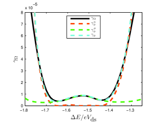
Figure 7: (Color online) Comparison of the linewidth $\gamma_{\Omega}$ of $S_{a,a^{\dagger}}(\omega)$ obtained from the $\lambda_{\Omega}$ eigenvalue (plotted as a function of $\Delta\tilde{E}$) with the analytic expression $\gamma_{\phi}=\gamma_{\phi}^{\phi}+\gamma_{\phi}^{n}$ (plotted as a function of $\Delta{E}$). Also shown are the direct ($\gamma_{\phi}^{\phi}$) and indirect ($\gamma_{\phi}^{n}$) phase diffusion contributions. Here $\kappa=0.03$, with other parameters the same as in Fig. 2.

V Current noise

In this section we investigate the extent to which features in the resonator noise spectra from Sec. III manifest themselves in the current noise. The low frequency limit of the current noise in this system was discussed in Ref. harvey:08, , but here our interest is in the dynamical timescales which become imprinted in the widths of the peaks in the finite frequency current noise. The finite frequency current noise through the SSET can be split into contributions from the current noise at the two junctions and the charge noise of the island,mozyrsky:02

$$S_{I,I}(\omega)=\frac{1}{2}S_{I_{L},I_{L}}(\omega)+\frac{1}{2}S_{I_{R},I_{R}}(\omega)-\frac{1}{4}\omega^{2}S_{Q,Q}(\omega),$$ (22)

where we have assumed equal junction capacitances. We choose the Cooper pair tunneling to take place at the left hand junction. To calculate the charge noise and the current noise at the left hand junction we can again use the quantum regression theorem as described in Sec. II.3,

$$S_{I_{L},I_{L}}(\omega) =4\Re\langle\!\langle l_{0}|\mathcal{I}_{L}\mathcal{R}(\omega)\mathcal{I}_{L}|r_{0}\rangle\!\rangle,$$

$$S_{Q,Q}(\omega) =4\Re\langle\!\langle l_{0}|\mathcal{Q}\mathcal{R}(\omega)\mathcal{Q}|r_{0}\rangle\!\rangle,$$ (23)

where the current and charge operators are defined as,

$$I_{L} =ie\frac{E_{J}}{\hbar}\Big{(}|2\rangle\langle 0|-|0\rangle\langle 2|\Big{)},$$

$$Q =e\Big{(}|1\rangle\langle 1|+2|2\rangle\langle 2|\Big{)}.$$ (24)

and the superoperator forms are defined in the same manner as Eq. (11). For the current noise at the right hand junction a counting variable approach can be used.flindt:05 The resulting expression is very much the same but with the addition of a self-correlation term,

$$S_{I_{R},I_{R}}(\omega)=2e\langle\!\langle l_{0}|\mathcal{I}_{R}|r_{0}\rangle\!\rangle+4\Re\langle\!\langle l_{0}|\mathcal{I}_{R}\mathcal{R}(\omega)\mathcal{I}_{R}|r_{0}\rangle\!\rangle,$$ (25)

where the current super operator for the right hand junction is defined,

$$\mathcal{I}_{R}|\rho(t)\rangle\!\rangle=e\Gamma\Big{(}|0\rangle\langle 1|\rho(t)|1\rangle\langle 0|+|1\rangle\langle 2|\rho(t)|2\rangle\langle 1|\Big{)}.$$ (26)

We give results in terms of the current Fano factor, $F_{I}(\omega)=S_{I,I}(\omega)/2e\left\langle I\right\rangle$. For the SSET alone the current noise spectrum, for these parameters, consists of a large peak at $\omega\simeq\Omega_{\rm SSET}$ and a much smaller peak at $\omega=0$.

In Figs. 8a and 8b we show the current noise spectra for the same off-resonant and resonant parameters used in Figs. 3a and 3b. The SSET current has a non-linear dependence on the resonator positionharvey:08 leading to peaks at higher harmonicsflindt:05a of $\Omega$. In the off-resonant regime the resonator state consists of Gaussian fluctuations about a fixed point and only the $\omega\simeq 2\Omega$ harmonic is seen in the current noisearmour:04 ; doiron:06 and it is very much weaker than the peak at $\omega\simeq\Omega$. On-resonance, the resonator motion consists of oscillations of a (relatively) much larger amplitude and hence leads to clearly visible peaks at higher harmonics of $\Omega$.

It is interesting to note that for the peak near $\omega\simeq\Omega$ the off-resonant current noise spectrum displays an important difference from the resonator spectra: as is shown in the inset (Fig. 8a) the peak is not of a Lorentzian form. The non-Lorentzian shape of this peak in the fixed point regime can be understoodrodrigues:08 as arising from an extra element of correlation between the SSET and resonator: the SSET current picks up the fluctuations in the resonator motion which were originally driven by the SSET charge motion (rather than a totally uncorrelated external bath).rodrigues:08 This effect is rapidly reduced with increasing external damping and temperature. Note that in the limit-cycle (resonant) region the peak at $\omega\simeq\Omega$ is again a Lorentzian.

Nevertheless, we find that the non-Lorentzian peak at $\omega\simeq\Omega$ in the fixed point regime can still be fitted by a term in the eigenfunction expansion Eq. 13 (but with a complex matrix element $m_{B}^{p}$), and hence the parameter describing the width, $\Re\lambda_{\Omega,I}$, can be obtained over the whole range of $\Delta E$. Comparing $\Re\lambda_{\Omega,I}$ obtained in this way with the linewidth $\gamma_{\phi}$, and comparing the width of the $\omega=0$ peak in $S_{I,I}(\omega)$ with $\gamma_{n}$ for the parameters in Fig. 4 we find in both cases that the pairs of curves overlay one another (the resulting plot thus effectively duplicates that shown in Fig. 4 and hence is not shown here). Hence the current noise provides a direct measure of the spectral properties of the resonator spectra and, in particular, gives access to the energy relaxation and phase diffusion rates.

Figure 8: (Color online) Finite frequency current noise spectrum for $\kappa=0.003$ with the other parameters the same as in Fig. 2. (a) Off-resonance $\Delta E=-1.75\,eV_{\rm ds}$, (b) on-resonance for $\Delta E=-1.59\,eV_{\rm ds}$. The insets show expansions of the narrow peaks at $\omega\simeq\Omega$ without logarithmic scaling (full lines) along with fits to the peaks (dashed lines) with the form of Eq. 13, inset (a), and Lorentzian form, inset (b).

VI Conclusions

We have studied the noise properties of a resonator coupled to a SSET in the vicinity of the JQP resonance, focussing our analysis on the case of a resonator whose frequency is large compared to the quasiparticle decay rate. We analyze the resonator spectrum that includes fluctuations in both the resonator energy and phase, $S_{a,a^{\dagger}}(\omega)$, as well as the spectrum of energy fluctuations $S_{n,n^{\dagger}}(\omega)$. The main feature in the spectrum $S_{a,a^{\dagger}}(\omega)$ is a large peak at the resonator frequency, $\omega\approx\Omega$ while $S_{n,n^{\dagger}}(\omega)$ is dominated by a peak at $\omega=0$. We find that outside transition regions, these peaks are Lorentzian with widths, $\gamma_{\Omega}$ (the linewidth) and $\gamma_{n}$, respectively, which are each controlled by a single eigenvalue of the Liouvillian. Examining the behavior of these eigenvalues for a range of coupling strengths, we find that for large enough coupling $\lambda_{\Omega}$ has a double minimum as a function of the detuning from resonance. An analysis of the coupled dynamics of the system allows us to identify the peak width $\gamma_{n}$ with the energy relaxation rate and $\gamma_{\Omega}$ (within the limit-cycle regime) with the phase diffusion rate. We show that the double minimum in the linewidth arises from a combination of direct and indirect phase diffusion. Finally, we show that these rates can be extracted from the current noise, and thus the current noise provides a direct measure of the key dynamical time scales of the resonator.

Appendix A Energy dependent damping and diffusion

In this appendix we present further details on the analytical approximations used to obtain the effective damping and diffusion rates. The details of the methods used in the calculations (and the approximations required) can be found in Refs. rodrigues:08a, and rodrigues:09, . Although the expressions obtained are only valid for small Josephson energy, $E_{J}\ll\hbar\Gamma$, they are valid for all values of $\Omega/\Gamma$, i.e. for both fast and slow resonators. The basis of the calculation is that the resonator energy is assumed to relax very slowly compared to both the resonator period and the quasiparticle tunneling rate, so that its effect on the SSET charge can be approximated as a harmonic drive. The behavior of the SSET under the influence of this drive is then found, and the result then fed back to obtain a coarse-grained equation of motion for the resonator.

The effective damping, $\gamma_{\rm eff}$, and frequency shift, $\Omega^{\prime}=\Omega_{R}-\Omega$, for a resonator with average (real) amplitude $\sqrt{E}$ are given by,rodrigues:08a

$$\frac{\gamma_{\rm eff}(E)}{2}+i\Omega^{\prime}(E) =-i\frac{x_{s}\Omega\pi^{2}E_{J}^{2}\Gamma^{2}}{x_{q}(eV_{ds})^{2}2\sqrt{E}}\frac{(3\Gamma+2i\Omega)}{(\Gamma+i\Omega)^{2}}$$

$$\times\sum\limits_{n}J_{n}(z)J_{1-n}(z)\left(\frac{1}{h_{n}}-\frac{1}{h_{-n}^{*}}\right)$$ (27)

where $x_{q}=\sqrt{\hbar/(2m\Omega)}$, the Bessel function of the first kind $J_{n}(z)$ is a function of the scaled amplitude $z=2\sqrt{E}x_{s}/x_{q}$ and we define $h_{n}=\frac{\Gamma}{2}+i(\Omega n+\Delta E/\hbar)$.

In a similar way, the fluctuations of the charge on the SSETrodrigues:08a lead to effective diffusion constants for the amplitude and phase of the resonator.rodrigues:09 The details of the calculation are rather involved, and the calculation follows the same approach as that given in Ref. rodrigues:09, hence here we merely summarize the results. The total diffusion rate is given by $D_{\rm eff}^{\pm}=\frac{E_{J}^{2}\Gamma^{4}}{(eV_{ds})^{2}}\pi^{3}\Omega\kappa\Re\left(D_{1}^{\pm}+D_{2}^{\pm}+D_{3}^{\pm}\right)$, where $D_{\rm eff}^{+}$ refers to the phase diffusion, and the $D_{\rm eff}^{-}$ terms to the amplitude diffusion. The first term is,

$$D_{1}^{\pm} =\frac{1}{2}\sum\limits_{n}\frac{\left|J_{n+1}(z)C_{1}\pm J_{n-1}(z)C_{1}^{*}\right|^{2}}{|h_{n}|^{2}},$$

where

$$C_{1}=\frac{3\Gamma+2i\Omega}{(\Gamma+i\Omega)^{2}}.$$

The second term is given by,

$$D_{2}^{\pm} =\sum\limits_{n}\frac{\left(J_{n+1}(z)C_{1}\pm J_{n-1}(z)C_{1}^{*}\right)}{h_{n}^{*}}$$

$$\times\left(\frac{J_{n+1}(z)C_{2}^{*}}{h_{n+1}^{*}}\pm\frac{J_{n-1}(z)C_{2}}{h_{n-1}^{*}}\right),$$

with

$$C_{2}=\frac{2\Gamma+i\Omega}{(\Gamma+i\Omega)^{2}}.$$

The final term is given by,

$$D_{3}^{\pm} =\sum\limits_{n}C_{3}J_{n}^{2}(z)\left(\frac{1}{h_{n}^{*}}+\frac{1}{h_{n}}\right)$$

$$\pm C_{4}J_{n-1}(z)J_{n+1}(z)\left(\frac{1}{h_{n-1}^{*}}+\frac{1}{h_{n+1}}\right)$$

where

$$C_{3} =\frac{5\Gamma^{2}+2\Omega^{2}}{(\Gamma^{2}+\Omega^{2})^{2}}$$

$$C_{4} =\frac{\Gamma C_{2}^{2}}{\Gamma+i2\Omega}+\frac{\Gamma^{2}}{(\Gamma+i\Omega)^{2}(\Gamma+i2\Omega)^{2}}.$$

The effective damping and diffusion can now be used to calculate the linewidth. These quantities can in addition be integrated to give an effective potential, allowing a calculation of the resonator distribution.rodrigues:09 We note that this result generalizes the phase diffusion rate calculated in Ref. bennett:06, to the regime where $\Omega/\Gamma$ is no longer small.

References

- (1) A. A. Clerk and S. Bennett, New J. Phys. 7 238 (2005).
- (2) M. P. Blencwoe, J. Imbers and A. D. Armour, New J. Phys. 7 236 (2005).
- (3) S. D. Bennett and A. A. Clerk, Phys. Rev. B 74, 201301(R) (2006).
- (4) D. A. Rodrigues, J. Imbers and A. D. Armour, Phys. Rev. Lett. 98 067204 (2007).
- (5) M. Marthaler, G. Schön and A. Shnirman, Phys. Rev. Lett. 101 147001 (2008).
- (6) T. J. Harvey, D. A. Rodrigues and A. D. Armour, Phys. Rev. B 78, 024513 (2008).
- (7) S. André, V. Brosco, A. Shnirman and G. Schön, Phys. Rev. A 79, 053848 (2009).
- (8) S. Ashhab, J. R. Johansson, A. M. Zagoskin and F. Nori, New J. Phys. 11, 023030 (2009).
- (9) O. Astafiev, K. Inomata, A. O. Niskanen , T. Yamamoto, Yu. A. Pashkin, Y. Nakamura and J. S. Tsai, Nature (London) 449 588 (2007).
- (10) A. Naik, O. Buu, M. D. LaHaye, A. D. Armour, A. A. Clerk, M. P. Blencowe and K. C. Schwab, Nature (London) 443 193 (2006).
- (11) V. Koerting, T. L. Schmidt, C. B. Doiron, B. Trauzettel and C. Bruder, Phys. Rev. B 79, 134511 (2009).
- (12) T. J. Kippenberg and K. J. Vahala, Science 321, 1172 (2008).
- (13) I. Favero and K. Karrai, Nature Photon. 3, 201 (2009).
- (14) F. Marquardt and S. M. Girvin, Physics 2 40 (2009).
- (15) D. A. Rodrigues, J. Imbers, T. J. Harvey and A. D. Armour, New J. Phys. 9 84 (2007).
- (16) J. Q. You, Y.-X. Liu, C. P. Sun and F. Nori, Phys. Rev. B 75, 104516 (2007).
- (17) B.-G. Englert and G. Morigi, in Coherent Evolution in Noisy Environments. Lecture Notes in Phys. (Springer, Berlin)”, 611, 55 (2002).
- (18) Yu. V. Nazarov and Ya. M. Blanter, Quantum Transport, (Cambridge University Press, Cambridge, UK), (2009).
- (19) V. Ya. Aleshkin and D. V. Averin, Physica B 165&166, 949 (1990).
- (20) M.-S. Choi, F. Plastina and R. Fazio, Phys. Rev. B 67, 045105 (2003).
- (21) J. Hauss, A. Fedorov, C. Hutter, A. Shnirman and G. Schön, Phys. Rev. Lett. 100, 037003 (2008).
- (22) K. Jaehne, K. Hammerer and M. Wallquist, New J. Phys. 10, 095019 (2008).
- (23) M. Lax, Phys. Rev. 160, 290 (1967).
- (24) D. F. Walls and G. J. Milburn, Quantum Optics, (Springer, Berlin, Germany), (1994).
- (25) K. Blum, Density Matrix Theory and Applications, (Plenum Press, New York), (1996).
- (26) H.-J. Briegel and B.-G. Englert, Phys. Rev. A 47, 3311 (1993).
- (27) M. Jakob and S. Stenholm, Phys. Rev. A 69, 042105 (2004).
- (28) C. Flindt, T. Novotný and A.-P. Jauho, Phys. Rev. B 70, 205334 (2004).
- (29) T. Brandes, Ann. Phys. 17, 477 (2008).
- (30) I. Djuric, B. Dong and H. L. Cui, J. Appl. Phys. 99, 063710 (2006).
- (31) R. B. Lehoucq, D. C. Sorensen and C. Yang, ARPACK Users’ Guide: Solution of Large-Scale Eigenvalue Problems with Implicitly Restarted Arnoldi Methods, (SIAM) (1998).
- (32) D. A. Rodrigues, Phys. Rev. Lett. 102 067202 (2009).
- (33) D. A. Rodrigues and G. J. Milburn, Phys. Rev. B 78, 104302 (2008).
- (34) M. Lax, Phys. Rev. 145, 110 (1966).
- (35) M. O. Scully and M. S. Zubairy, Quantum Optics, (Cambridge University Press, Cambridge, UK), (1997).
- (36) D. A. Rodrigues and A. D. Armour, arXiv:0909.4389 (2009).
- (37) D. Mozyrsky, L. Fedichkin, S. A. Gurvitz and G. P. Berman, Phys. Rev. B 66, 161313(R) (2002).
- (38) C. Flindt, T. Novotný and A.-P. Jauho, Europhys. Lett. 69, 475 (2005).
- (39) C. Flindt, T. Novotný and A.-P. Jauho, Physica E 29 411 (2005).
- (40) A. D. Armour, Phys. Rev. B 70, 165315 (2004).
- (41) C. B. Doiron, W. Belzig and C. Bruder, Phys. Rev. B 74, 205336 (2006).