Quantifying structure in networks

Abstract

We investigate exponential families of random graph distributions as a framework for systematic quantification of structure in networks. In this paper we restrict ourselves to undirected unlabeled graphs. For these graphs, the counts of subgraphs with no more than $k$ links are a sufficient statistics for the exponential families of graphs with interactions between at most $k$ links. In this framework we investigate the dependencies between several observables commonly used to quantify structure in networks, such as the degree distribution, cluster and assortativity coefficients.

1 Introduction

The notion of “complex networks” is usually utilized in an informal manner, intending to suggest that these networks are not simple in some sense or another. Among the simple networks one would include regular lattices on the one side and purely random networks, i.e. Erdős-Rényi random graphs or Bernoulli graphs, on the other side. In contrast, in the physics literature, two types of networks are considered as prototypes of complex networks: scale free graphs, i.e. graphs with degrees distributed according to a power law and small world networks, i.e. graphs with a small diameter, but higher cluster coefficient than a Bernoulli graph with the same diameter. Thus the degree distribution and the cluster coefficient are used to define certain kinds of complex networks. Another structural property, utilized to assess whether some graph should be termed complex, is its assortativity or disassortativity, describing whether high degree nodes are more often connected to high degree nodes or to low degree nodes.

These properties are not independent of each other; the degree distribution, for instance, imposes constraints on the degree of assortativity. Therefore it would be desirable to have a general framework that allows to study these dependencies in a systematic way and, in particular, to quantify structure and therefore complexity of networks. Here we propose the theory of hierarchically structured exponential families Amari2001 ; Kahle2009 with the help of which we can, starting from the Erdős-Rényi random graphs, incorporate more and more interaction between parts of a network and provide a framework for quantifying the degree of interaction.

In this theory “complexity” means statistical complexity Ay2006b : In order to distinguish between the structure and the random part, not only one object is considered, but a set of objects equipped with a probability distribution. “Random” then means statistically independent. Accordingly, measures of statistical complexity quantify statistical dependencies in a distribution. They vanish in both cases of a totally ordered and a totally random system.

Using the notion of “statistical complexity” to characterize single objects such as a given network is problematic in the following sense. If we speak about the complexity of a single network, we have to consider it as typical in an ensemble of networks. This assumption need not always be justified. If it is satisfied, however, we can use an ergodicity-type argument to approximate ensemble means by counts over a single typical instance in the ensemble. For example, the count of edges in one instance should provide an estimate of the edge probability in the ensemble.

This paper is structured as follows. In Section 2 we describe the theoretical framework of exponential families of random graphs. Building on this, Section 3 contains our main results. We interpret common observables on graphs in our framework and shed new light on their interpretation. Section 4 contains concrete examples of our models with few parameters and discusses special features of sampling procedures. Following the discussion in Section 5 is an Appendix which contains technical details.

2 Basic setting — exponential families of random graphs

We consider undirected random graphs without self connections, specified by an adjacency matrix $A$. Denote by $N$ the number of nodes, $[N]\mathrel{\mathop{:}}=\left\{1,\ldots,N\right\}$ the set of nodes, and $E\mathrel{\mathop{:}}=\left\{(i,j)\in[N]\times[N]:i\neq j\right\}$ the set of off-diagonal indices of $A$. In a given graph each edge is either present or not, therefore we are dealing with $\left\lvert E\right\rvert$ binary random variables. Denote by $\mathcal{X}\mathrel{\mathop{:}}=\left\{0,1\right\}^{E}$ the set of states of this collection of random variables. For any subset $B$ of potential edges we denote $\mathcal{X}_{B}\mathrel{\mathop{:}}=\left\{0,1\right\}^{B}$.

In this labeled setting the probability of a random graph is given by the probability of its adjacency matrix $A=(a_{e})_{e\in E}$. A random graph $G$ is described by binary random variables with state space $\mathcal{X}$ and a probability

$$P(G)=P(a_{e_{1}},\ldots,a_{e_{N(N-1)}})\;.$$

A distribution $P(G)$ is often called a graph ensemble in the following. We consider so called exponential families, classes of graph ensembles with a particularly nice structure and interpretation. When used to describe probability distributions for random graphs they have been termed “exponential random graphs”, “$p^{*}$ models”, or “logit-models” in the literature. For a recent overview see Robins2007 . Here, we utilize families $\mathcal{E}_{k}$ that consist of the distributions with interactions between at most $k$ units. Let $f$ be a function mapping states $(a_{e_{1}},\ldots,a_{e_{N(N-1)}})$ to the reals. With the usual addition and multiplication by real numbers, these functions form a vector space

$$\mathbb{R}^{\mathcal{X}}\mathrel{\mathop{:}}=\left\{f:\mathcal{X}\to\mathbb{R}\right\}.$$

Of course, any (real-valued) observable is such a function. Our systematic approach to quantifying structure consists in considering natural bases of this space. We can then express well known observables in terms of these bases, yielding a better understanding of the relation between observables.

The probability measures

$$\mathcal{P}(\mathcal{X})\mathrel{\mathop{:}}=\left\{P\in\mathbb{R}^{\mathcal{X}}:P(x)>0,\sum_{x\in\mathcal{X}}P(x)=1\right\}\;,$$

form a subset of $\mathbb{R}^{\mathcal{X}}$, which has the geometry of a simplex. Its closure, where $P(x)=0$ is allowed, is denoted by $\overline{\mathcal{P}}(\mathcal{X})$. The exponential map assigns to each function a strictly positive probability measure:

$$\exp:\mathbb{R}^{\mathcal{X}}\to\mathcal{P}(\mathcal{X})\qquad f\mapsto\frac{\exp(f)}{\sum_{x\in\mathcal{X}}\exp(f(x))}\;.$$

Here, $\exp(f)$ is to be taken coordinatewise. Using the exponential map, there is a natural way to define exponential families of probability measures by considering families $\mathcal{E}$ that are exponential images of linear subspaces of $\mathbb{R}^{\mathcal{X}}$. One natural class of such subspaces is given by limiting the interaction order. Following Ay2006a ; Kahle2009 one can define

$${\mathcal{I}}_{B}\mathrel{\mathop{:}}=\left\{f\in{\mathbb{R}}^{\mathcal{X}}:f(x_{B},x_{E\setminus B})=f(x_{B},x_{E\setminus B}^{\prime})\mbox{ for all $x_{B}\in\mathcal{X}_{B}$, $x_{E\setminus B},x_{E\setminus B}^{\prime}\in\mathcal{X}_{E\setminus B}$}\right\}\;,$$

as the space of functions depending only on the subset $B\subseteq E$ of their arguments. Then

$$\mathcal{I}_{k}=\sum_{\left\lvert B\right\rvert\leq k}\mathcal{I}_{B}$$

is the space of functions depending on at most $k$ of their arguments. Here, the sum over $\mathcal{I}_{B}$ is to be understood as their span inside $\mathbb{R}^{\mathcal{X}}$. This definition leads to a hierarchy of exponential families

$$\mathcal{E}_{1}\subsetneq\ldots\subsetneq\mathcal{E}_{N(N-1)-1}\subsetneq\mathcal{P}(\mathcal{X})\;,$$ (1)

which is studied in information geometry Amari2001 . It allows to model networks by considering interactions of successively increasing order between their parts. It has been used to quantify the amount and degree of interaction in dynamical systems in a systematic fashion in Kahle2009 .

The notion of interaction order can be understood from the fact that any $P\in\mathcal{E}_{k}$ has a (non-unique) representation as

$$P(G)=\prod_{B\subseteq E:\left\lvert B\right\rvert=k}\Phi(x_{B})=\frac{1}{Z}\exp\left(\sum_{B\subseteq E:\left\lvert B\right\rvert=k}\phi_{B}(x_{B})\right)\;.$$

Thus, $P\in\mathcal{E}_{k}$ means that

$$P(G)= \frac{1}{Z}e^{-\mathcal{H}(G)}$$

$$\mathcal{H}(G)= \sum_{e}c_{e}f_{e}(a_{e})+\sum_{e_{1},e_{2}}c_{e_{1},e_{2}}f_{e_{1},e_{2}}(a_{e_{1}},a_{e_{2}})+\ldots$$ (2)

$$\ldots+\sum_{e_{1},e_{2},\ldots,e_{k}}c_{e_{1},e_{2},\ldots,e_{k}}f_{e_{1},e_{2},\ldots,e_{k}}(a_{e_{1}},a_{e_{2}},\ldots,a_{e_{k}})\;.$$

As mentioned above any collection $\mathcal{O}_{1},\ldots,\mathcal{O}_{s}$ of observables defines a linear space as their span

$$\mathcal{L}=\left\{f\in\mathbb{R}^{\mathcal{X}}:f=\sum_{i=1}^{s}c_{i}\mathcal{O}_{i},\;c_{1},\ldots,c_{s}\in\mathbb{R}\right\}\;,$$

which in turn defines an exponential family $\mathcal{E}_{\mathcal{L}}\mathrel{\mathop{:}}=\exp(\mathcal{L})$. This exponential family is the collection of maximum entropy distributions for fixed expectation values of the observables. In particular, the mean values of the observables in a sample form a sufficient statistics for the model $\mathcal{E}_{\mathcal{L}}$. Given data, one can determine the mean values of the observables on the data and then find a unique $P$ in the closure $\overline{\mathcal{E}}_{\mathcal{L}}$ which has the same statistics as the data and maximal entropy among all such distributions. Finding this estimate in practice can be computationally expansive for a general linear space. In practice, an algorithm called iterative proportional fitting is used deming40 . It is implemented in cipi cipi and statistical software packages like loglin inside the software R. Since this method works directly on the vectors in $\mathbb{R}^{\mathcal{X}}$ it is limited to small $\mathcal{X}$. Less than $N=20$ elements can be feasible. It is well known that for $\mathcal{E}_{1}$ the maximum entropy distribution is just the product of the one-dimensional marginals of the data.

2.1 Undirected Graphs and subgraph counts

In the following we specialize the general theory to the case of undirected unlabeled homogeneous graphs. Here $E=\left\{(i,j)\in[N]\times[N]:i<j\right\}$ is the set of potential edges, resulting in a symmetric adjacency matrix $A=(a_{ij})_{i,j=1,\ldots,N}$, by setting $a_{ij}=a_{e}$ if $(i,j)\in E$ or $(j,i)\in E$, and $a_{ii}=0$.

Unlabeled graphs are defined as equivalence classes and working with them in practice becomes infeasible quickly. It is a curiosity of complexity theory that the graph isomorphism problem is in the class NP, but neither known to lie in P, nor to be NP-complete. In any case, at the current time there is no fast algorithm to determine whether two unlabeled graphs are isomorphic. Due to this unavoidable restriction we will always work with adjacency matrices. In particular the partition function is a sum over symmetric adjacency matrices and $P(H)$, for some unlabeled graph $H$ denotes the sum of probabilities of adjacency matrices which have $H$ as their unlabeled graph. This is complemented by the homogeneity that we assume in this setting. It means that we consider observables that are only evaluated on a small part of the system, and the value should show no systematic differences when varying the position. In particular, the probability of finding an edge should be the same for any pair of vertices. In the setting that was described in Section 2 this homogeneity is a certain symmetry requirement. For instance the Erdős-Rényi graphs emerge from the exponential family where the linear space is the one-dimensional span of the edge count observable.

Generalizing from Erdős-Rényi graphs to higher dependency structures, natural observables are the subgraph counts, defined as follows: Given a graph $G$ with potential edge set $E$, we define the subgraph counts of a subgraph $H$ as

$$n_{H}\mathrel{\mathop{:}}=\#\left\{\text{unlabeled subgraphs $H$ of $G$}\right\}\;.$$ (3)

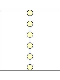
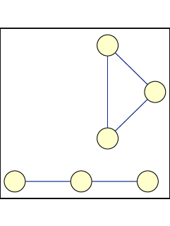
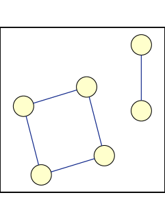
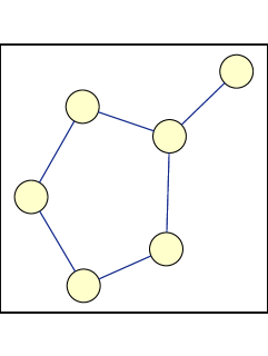
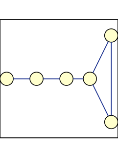
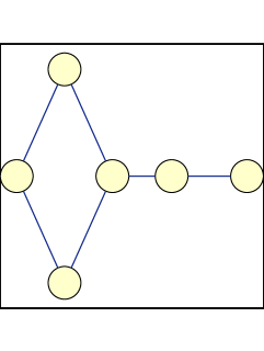
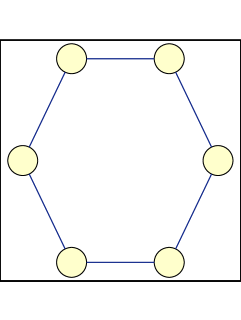
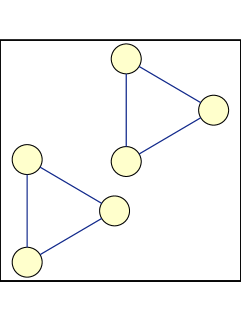
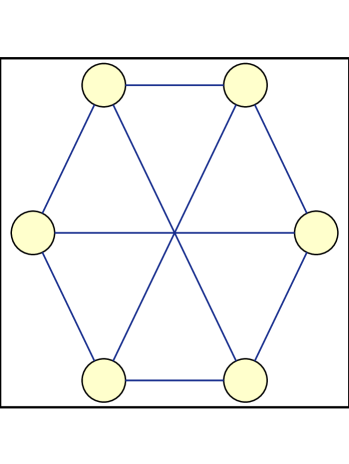
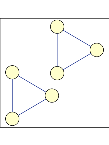
For example, we denote by $n_{-}$ the number of edges and by $n_{\includegraphics[height=3.01389pt]{9.pdf}}$ the number of triangles. For any undirected graph $G$, the counts of subgraphs with at most $k$ edges form a sufficient statistics for the exponential family $\mathcal{E}_{k}$ considered above. This can be seen as follows. For each set $B\subseteq E$ of potential edges, we can define a function which takes the value one precisely if all edges in $B$ are present, i.e. it counts the subgraph defined by the labeled graph $B$:

$$f_{B}(G):=\prod_{e\in B}a_{e}\;.$$ (4)

A classical argument from the theory of Markov random fields winkler_image_analysis shows that these functions $\left\{f_{B}:B\subseteq E\right\}$ form a basis of the whole space $\mathbb{R}^{\mathcal{X}}$, while with $k=\left\lvert B\right\rvert$ we have $f_{B}\in\mathcal{I}_{k}$. Uniqueness of the coefficients with respect to this basis depends on a choice of a reference configuration, the so called vacuum state. In our case the vacuum is the empty graph. The statement about sufficiency follows if one observes that the homogeneity requirement translates into a condition on the coefficients in (2): Coefficients $c_{e_{1},\ldots,e_{l}}$ for different $e_{1},\ldots,e_{l}$ representing the same undirected unlabeled subgraph are required to be the same. Therefore the counts of unlabeled subgraphs with $k$ edges (which are just sums over the $f_{B}$ for all $B$ representing a specific subgraph) span the linear subspace space of functions depending only on $k$ of their arguments, and taking equal values whenever these $k$ arguments represent the same subgraph. Summarizing we have

$$\sum_{B\sim H}f_{B}=n_{H}\;,$$ (5)

where the summation runs over all sets $B$ which define a subgraph isomorphic to an unlabeled graph $H$.

Note that fixing the number of vertices breaks the relation with the hierarchy in (1). Consider as an example the full model with subgraph counts up to 4 vertices. The energy has the form

$$\mathcal{H}=c_{-}n_{-}+c_{\includegraphics[height=3.01389pt]{2.pdf}}n_{\includegraphics[height=3.01389pt]{2.pdf}}+c_{\includegraphics[height=3.01389pt]{9.pdf}}n_{\includegraphics[height=3.01389pt]{9.pdf}}+\ldots+c_{\includegraphics[height=3.01389pt]{6.pdf}}n_{\includegraphics[height=3.01389pt]{6.pdf}}+c_{\includegraphics[height=3.01389pt]{7.pdf}}n_{\includegraphics[height=3.01389pt]{7.pdf}}\;.$$ (6)

This distribution is an element of $\mathcal{E}_{6}$, but not all elements of $\mathcal{E}_{6}$ are of this form, as we have not used a subgraph count for 6 edges forming a chain, which would be a subgraph on 7 vertices. It is also important to notice that changing one of the coefficients will generally change all of the expected counts.

Apart from the subgraph counts, we often use the subgraph probabilities $p_{H}$, that is, the probabilities for observing the subgraph $H$ when drawing a random graph from the ensemble $P$ on randomly selected nodes. This can be written as an expectation value with respect to the distribution $P$ as

$$p_{H}\mathrel{\mathop{:}}=\left\langle f_{B}\right\rangle,\qquad B\sim H\;,$$ (7)

where $B\subseteq E$ is any set of edges whose unlabeled graph is $H$. That any such $B$ can be chosen is a consequence of the homogeneity that we require for our model. If the subgraphs whose counts we use as observables are small enough (when compared to the size of the network $G$), the homogeneity assumption allows to use counts on a single given network to estimate the ensemble expectation values. Quantities derived from a single network are denoted by a hat as in $\widehat{n}_{H}$.

When a subgraph probability $p_{H}$ is estimated from a single network, it is given by the count of that subgraph, normalized by the maximum possible number of occurrences of that subgraph. This in turn is just the number of occurrences of $H$ in the fully connected network $F$:

$$\widehat{p}_{H}=\frac{n_{H}(G)}{n_{H}(F)}\;.$$ (8)

3 Measures of structural network properties

3.1 Link density

One of our main aims is to find good sets of network observables that capture the important structural properties of a graph. Obviously the first property is the number of links $n_{-}$ or the link density

$$\widehat{p}_{-} = \frac{n_{-}(G)}{n_{-}(F)}$$ (9)

$$= \frac{2n_{-}}{N(N-1)}\;,$$ (10)

with $F$ denoting the fully connected graph.
If only the expectation value of the link density or the number of links is specified, the corresponding maximum entropy ensemble is the ensemble of Erdős-Rényi random graphs or Bernoulli graphs. Its Hamiltonian is simply

$$\mathcal{H}(G)=c_{-}n_{-}=c_{-}\sum_{(i,j):i<j}a_{ij}\;.$$ (11)

The main property of this ensemble is that there are no statistical dependencies between the links. The degrees of the nodes are distributed according to a Bernoulli distribution fully determined by the mean node degree.

3.2 Degree distribution

A distribution different from the Bernoulli distribution introduces statistical dependencies between the potential links. The resulting random graph ensemble will therefore be different from the Bernoulli graphs. How does the degree enter our framework? In a first step one might label the nodes using some labeling $\pi$, and assign to each node an expected degree. This leads to exponential random graph model

$$\mathcal{H}(G,\pi)=\sum_{i}c_{i}\sum_{j}a_{\pi(i)\pi(j)},$$ (12)

with the $c_{i}$ determining the degree of node $\pi(i)$. In a second step one considers an ensemble of ensembles of random graphs, where the different ensembles correspond to different labellings, i.e. permutations of the node degrees. This leads to a probability distribution that is a convex combination of distributions $P\in\mathcal{E}_{1}$, and thus generally not contained in $\mathcal{E}_{1}$ but in a so called mixture model. Moreover, this approach does not lead to a parameterization of the form (2).

Our next aim is to understand how the degree distribution can be specified within the exponential families $\mathcal{E}_{k}$. The key point is that the $k$-star counts allow to determine the moments of the degree distribution. With $d_{i}=\sum_{j}a_{ij}$ being the degree of node $i$ we call $P(d)$ the probability that a randomly chosen node has degree $d$. We find

$$P(d) = \sum_{G}P(G)\frac{1}{N}\sum_{i=1}^{N}\delta_{d_{i}(G),d}\;.$$ (13)

The moments of the degree distribution are

$$\mu_{k}=\langle d^{k}\rangle=\sum_{d=0}^{\infty}d^{k}P(d)\;.$$ (14)

For a given graph, we also have the empirical degree distribution

$$\widehat{P}_{G}(d)=\frac{1}{N}\sum_{i=1}^{N}\delta_{d_{i}(G),d}\;,$$

with the moments

$$\widehat{\mu}_{k}=\frac{1}{N}\sum_{i=1}^{N}d_{i}^{k}\;.$$ (15)

Note that $\langle\widehat{\mu}_{k}\rangle=\mu_{k}$. There is a direct relationship between the moments of the degree distribution and the numbers of $k$-stars

$$n_{k}=\sum_{i=1}^{N}{d_{i}\choose k}\;.$$ (16)

Note that with this definition the number of $1$-stars is two times the numbers of links $n_{1}=2n_{-}$. Thus looking for the maximum entropy distribution for graphs with given moments of the degree distribution up to order $k_{\max}$ corresponds to the exponential random graph model having non-zero coefficients only for $k$-stars with $k\leq k_{\max}$. In particular, this distribution lies in $\mathcal{E}_{k_{\max}}$. The parameterization using the $k$-stars on the one hand side

$$\mathcal{H}=\sum_{k=1}^{k_{\max}}c_{k}n_{k}\;,$$ (17)

and the moments of the empirical degree distribution of the graph

$$\mathcal{H}=\sum_{k=1}^{k_{\max}}c^{(d)}_{k}\widehat{\mu}_{k}\;,$$ (18)

can be converted into each other using

$$n_{k} = \frac{1}{k!}\sum_{i=1}^{N}\sum_{m=1}^{k}s(k,m)d_{i}^{m}$$ (19)

$$= \frac{N}{k!}\sum_{m=1}^{k}s(k,m)\widehat{\mu}_{m}\;.$$ (20)

with $s(k,m)$ being the Stirling numbers of the first kind. The inverse relationship between the $k$-star counts and the moments of the degree distribution can be expressed using the Stirling number of the second kind $S(k,m)$:

$$\widehat{\mu}_{k}=\sum_{m=1}^{k}S(k,m)\frac{k!}{N}n_{m}\;.$$ (21)

For the parameters this leads to the relationships

$$c_{m} = \sum_{k=m}^{k_{\max}}\frac{k!}{N}S(k,m)c^{(d)}_{k}$$ (22)

$$c^{(d)}_{m} = \sum_{k=m}^{k_{\max}}\frac{N}{k!}s(k,m)c_{k}\;.$$ (23)

The parameterization (18) might still not be the best way to explore different degree distributions, because of the dependencies between the different moments. Instead of using the empirical moments (15) as observables, one could think of observables that can be independently varied more easily, such as the variance, skewness, and kurtosis. Let us look in more detail at the variance, the other cases are similar. In the two star model

$$\mathcal{H}(G) = c_{-}n_{-}+c_{\includegraphics[height=3.01389pt]{2.pdf}}n_{\includegraphics[height=3.01389pt]{2.pdf}}$$ (24)

$$= c_{1}n_{1}+c_{2}n_{2}\;.$$ (25)

with $c_{1}=c_{-}/2$ and $c_{2}=c_{\includegraphics[height=3.01389pt]{2.pdf}}$, the resulting probability distribution can be equivalently parameterized by the pairs $(c_{1},c_{2})$, $(\mu_{1},\mu_{2})$ or $(\mu_{1},\mu_{2}-\mu_{1}^{2})$, the last being the mean and the variance of the degree distribution. The variance of the empirical degree distribution of a graph $G$ is

$$\mbox{var}(\widehat{P}(d))=\widehat{\mu}_{2}-{\widehat{\mu}_{1}}^{2}\;.$$ (26)

One might think of a Hamiltonian of the form

$$\mathcal{H}(G)=c^{(d)}_{1}\widehat{\mu}_{1}+\widetilde{c}^{(d)}_{2}\left(\widehat{\mu}_{2}-{\widehat{\mu}_{1}}^{2}\right)\;.$$ (27)

This model is different from the two star model because it involves a non-linear transformation of the observables.

3.3 Cluster coefficient

The cluster coefficient can be defined as three times the ratio between the numbers of triangles and the numbers of two stars in a given graph:

$$\widehat{C} = \frac{3n_{\includegraphics[height=3.01389pt]{9.pdf}}}{n_{\includegraphics[height=3.01389pt]{2.pdf}}}$$ (28)

$$= \frac{\widehat{p}_{\includegraphics[height=3.01389pt]{9.pdf}}}{\widehat{p}_{\includegraphics[height=3.01389pt]{2.pdf}}}\;,$$ (29)

with

$$\widehat{p}_{\includegraphics[height=3.01389pt]{2.pdf}} = \frac{2n_{\includegraphics[height=3.01389pt]{2.pdf}}}{N(N-1)(N-2)}$$ (30)

$$\widehat{p}_{\includegraphics[height=3.01389pt]{9.pdf}} = \frac{6n_{\includegraphics[height=3.01389pt]{9.pdf}}}{N(N-1)(N-2)}\;.$$ (31)

Thus the cluster coefficient for the ensemble $P$ measures the conditional probability that if for three randomly selected nodes one node is connected to the two others, these are also connected.

$$C=p(a_{ij}=1|a_{ik}=1,a_{jk}=1)\;.$$ (32)

In the context of social networks this property is also called “transitivity” because it means the probability that the friend of my friend is also my friend. If there are no statistical dependencies between the links, we would expect

$$C_{\text{ind}}:=p_{-}\;.$$ (33)

Moreover, if there are statistical dependencies only between pairs of links ($P(G)\in\mathcal{E}_{2}$), such as in the two star model, one might expect

$$p(a_{ij}=1|a_{ik}=1,a_{jk}=1)=p(a_{ij}=1|a_{ik}=1)\;,$$

or

$$\frac{p_{\includegraphics[height=3.01389pt]{9.pdf}}}{p_{\includegraphics[height=3.01389pt]{2.pdf}}}=\frac{p_{\includegraphics[height=3.01389pt]{2.pdf}}}{p_{-}},$$ (34)

respectively, and therefore the cluster coefficient would be equal to

$$\frac{p_{\includegraphics[height=3.01389pt]{2.pdf}}}{p_{-}}\;.$$ (35)

This is, however, not the correct expression for the two star model. Already the case of only three nodes provides an example:

$$P(G)=P(a_{1,2},a_{2,3},a_{3,1})=\frac{1}{Z}\exp(c_{-}n_{-}+c_{\includegraphics[height=3.01389pt]{2.pdf}}n_{\includegraphics[height=3.01389pt]{2.pdf}})\;.$$

There we have

$$ZP(0,0,0) = 1$$

$$ZP(1,0,0) = ZP(0,1,0)=ZP(0,0,1)=h_{1}=\exp c_{-}$$

$$ZP(1,1,0) = ZP(1,0,1)=ZP(0,1,1)=h_{2}=\exp(2c_{-}+c_{\includegraphics[height=3.01389pt]{2.pdf}})$$

$$ZP(1,1,1) = h_{3}=\exp(3c_{-}+3c_{\includegraphics[height=3.01389pt]{2.pdf}})=p_{\includegraphics[height=3.01389pt]{9.pdf}}$$

$$Z = 1+3h_{1}+3h_{2}+h_{3}\;.$$

Hence, the cluster coefficient is

$$C = \frac{p_{\includegraphics[height=3.01389pt]{9.pdf}}}{p_{\includegraphics[height=3.01389pt]{2.pdf}}}=\frac{P(1,1,1)}{P(1,1)}=\frac{P(1,1,1)}{P(1,1,1)+P(1,1,0)}$$

$$= \frac{h_{3}}{h_{2}+h_{3}}=\frac{1}{1+h_{2}/h_{3}}\;.$$

On the other hand (35) becomes

$$\frac{p_{\includegraphics[height=3.01389pt]{2.pdf}}}{p_{-}} = \frac{h2+h3}{h2+h3+h2+h1}$$

$$= \frac{1}{1+h_{2}/h_{3}(\frac{h_{1}/h_{2}+1}{h_{2}/h_{3}+1})}\neq C\;.$$

If the three random variables are only a subset of a larger set of random variables as in the case of larger networks, things become even more complicated.
Nevertheless, if $n_{-}$ and $n_{\includegraphics[height=3.01389pt]{2.pdf}}$ are sufficient statistics for the two star model, we should be able to express the cluster coefficient by these two variables. In particular, we should be able to express the expected number of triangles by the expected number of two stars and the expected number of links.

3.4 Markov graphs

If the Hamiltonian contains only the numbers of $k$-stars and triangles, it defines the so called Markov graphs Frank1986 . This class of random graphs is well known in the social network community. “Markov” here refers to the fact that in these graphs the occurrence of links without a common node is statistically independent. The only subgraphs where all pairs of links have a common node are the $k$-stars and the triangles. From what we have discussed so far it becomes clear that these models can account already for a large range of degree distributions in contrast to the statement sometimes found in the literature that the exponential random graph models of the social network community only accounts for Poissonian degree distributions Boerner2007 .

3.5 Assortativity

Another widely studied property of a graph is its assortativity or disassortativity. In an assortative graph, high degree nodes are prevalently connected to other high degree nodes and low degree nodes to low degree ones. In disassortative graphs, high degree nodes tend to be connected to low degree nodes. A simple way to measure this property is the correlation coefficient between the remaining degrees of two connected nodes Newman2002 . “Remaining” degree refers to the degree of a node after subtracting one for the link connecting this node to the other one. Empirical investigations showed that most social networks are assortative, while the Internet or biological networks are rather disassortative Newman2002 .

For an edge $a_{ij}=1$ the remaining degrees at either side of the edge are given by

$$d^{r,i}_{ij} = \sum_{k\neq i,j}a_{ki}=d_{i}-1\;,$$

$$d^{r,j}_{ij} = \sum_{l\neq i,j}a_{jl}=d_{j}-1\;.$$

The assortativity is then given by the correlation coefficient between the remaining degrees at either side of an edge:

$$r^{2}=\frac{\langle(d^{r,i}-\langle d^{r,i}\rangle)(d^{r,j}-\langle d^{r,j}\rangle)\rangle}{\sqrt{\langle(d^{r,i}-\langle d^{r,i}\rangle)^{2}\rangle\langle(d^{r,j}-\langle d^{r,j}\rangle)^{2}\rangle}}\;.$$

Using that we consider undirected graphs, i.e. $A$ is symmetric, $\langle(d^{r,i})^{n}\rangle=\langle(d^{r,j})^{n}\rangle$ for $n=1,2,\ldots$, and linearity of expectation values, this simplifies to

$$r^{2}=\frac{\langle d^{r,i}d^{r,j}\rangle-\langle d^{r,i}\rangle\langle d^{r,i}\rangle}{\langle(d^{r,i})^{2}\rangle-\langle d^{r,i}\rangle^{2}}\;.$$ (36)

All relevant quantities can now be expressed in terms of subgraph counts (see appendix for details):

$$\widehat{r^{2}}=\frac{\frac{n_{-}}{n_{\includegraphics[height=2.15277pt]{2.pdf}}}\left(\frac{3n_{\includegraphics[height=2.15277pt]{9.pdf}}}{n_{\includegraphics[height=2.15277pt]{2.pdf}}}+\frac{n_{\includegraphics[height=2.15277pt]{3.pdf}}}{n_{\includegraphics[height=2.15277pt]{2.pdf}}}\right)-1}{\frac{n_{-}}{n_{\includegraphics[height=2.15277pt]{2.pdf}}}\left(\frac{3n_{\includegraphics[height=2.15277pt]{4.pdf}}}{n_{\includegraphics[height=2.15277pt]{2.pdf}}}+1\right)-1}\;.$$ (37)

In order to express the assortativity by the subgraph probabilities we list again all subgraph probabilities including the missing ones:

$$\widehat{p}_{-} = \frac{2n_{-}}{N(N-1)}$$ (38)

$$\widehat{p}_{\includegraphics[height=3.01389pt]{2.pdf}} = \frac{2n_{\includegraphics[height=3.01389pt]{2.pdf}}}{N(N-1)(N-2)}$$ (39)

$$\widehat{p}_{\includegraphics[height=3.01389pt]{9.pdf}} = \frac{6n_{\includegraphics[height=3.01389pt]{9.pdf}}}{N(N-1)(N-2)}$$ (40)

$$\widehat{p}_{\includegraphics[height=3.01389pt]{4.pdf}} = \frac{6n_{\includegraphics[height=3.01389pt]{4.pdf}}}{N(N-1)(N-2)(N-3)}$$ (41)

$$\widehat{p}_{\includegraphics[height=3.01389pt]{3.pdf}} = \frac{2n_{\includegraphics[height=3.01389pt]{3.pdf}}}{N(N-1)(N-2)(N-3)}$$ (42)

Thus

$$\widehat{r^{2}} = \frac{\frac{\widehat{p}_{-}}{(N-2)\widehat{p}_{\includegraphics[height=2.15277pt]{2.pdf}}}\left(\frac{\widehat{p}_{\includegraphics[height=2.15277pt]{9.pdf}}}{\widehat{p}_{\includegraphics[height=2.15277pt]{2.pdf}}}+\frac{(N-3)\widehat{p}_{\includegraphics[height=2.15277pt]{3.pdf}}}{\widehat{p}_{\includegraphics[height=2.15277pt]{2.pdf}}}\right)-1}{\frac{\widehat{p}_{-}}{(N-2)\widehat{p}_{\includegraphics[height=2.15277pt]{2.pdf}}}\left(\frac{(N-3)\widehat{p}_{\includegraphics[height=2.15277pt]{4.pdf}}}{\widehat{p}_{\includegraphics[height=2.15277pt]{2.pdf}}}+1\right)-1}$$ (43)

$$= \frac{\left(\frac{\widehat{p}_{\includegraphics[height=2.15277pt]{9.pdf}}}{\widehat{p}_{\includegraphics[height=2.15277pt]{2.pdf}}}-\frac{\widehat{p}_{\includegraphics[height=2.15277pt]{2.pdf}}}{\widehat{p}_{-}}\right)+\left(\frac{\widehat{p}_{\includegraphics[height=2.15277pt]{3.pdf}}}{\widehat{p}_{\includegraphics[height=2.15277pt]{2.pdf}}}-\frac{\widehat{p}_{\includegraphics[height=2.15277pt]{2.pdf}}}{\widehat{p}_{-}}\right)(N-3)}{\left(1-\frac{\widehat{p}_{\includegraphics[height=2.15277pt]{2.pdf}}}{\widehat{p}_{-}}\right)+\left(\frac{\widehat{p}_{\includegraphics[height=2.15277pt]{4.pdf}}}{\widehat{p}_{\includegraphics[height=2.15277pt]{2.pdf}}}-\frac{\widehat{p}_{\includegraphics[height=2.15277pt]{2.pdf}}}{\widehat{p}_{-}}\right)(N-3)}\;.$$

The assortativity coefficient is zero, if

$$\frac{3\cdot n_{\includegraphics[height=3.01389pt]{9.pdf}}}{n_{\includegraphics[height=3.01389pt]{2.pdf}}}+\frac{n_{\includegraphics[height=3.01389pt]{3.pdf}}}{n_{\includegraphics[height=3.01389pt]{2.pdf}}}=\frac{n_{\includegraphics[height=3.01389pt]{2.pdf}}}{n_{-}}\;,$$ (44)

or equivalently

$$\frac{\widehat{p}_{\includegraphics[height=3.01389pt]{9.pdf}}}{\widehat{p}_{\includegraphics[height=3.01389pt]{2.pdf}}}+\frac{(N-3)\widehat{p}_{\includegraphics[height=3.01389pt]{3.pdf}}}{\widehat{p}_{\includegraphics[height=3.01389pt]{2.pdf}}}=\frac{(N-2)\widehat{p}_{\includegraphics[height=3.01389pt]{2.pdf}}}{\widehat{p}_{-}}\;,$$ (45)

which is a relation between conditional probabilities that is fulfilled in particular if

$$\frac{\widehat{p}_{\includegraphics[height=3.01389pt]{3.pdf}}}{\widehat{p}_{\includegraphics[height=3.01389pt]{2.pdf}}}=\frac{\widehat{p}_{\includegraphics[height=3.01389pt]{2.pdf}}}{\widehat{p}_{-}}\quad\text{ and }\quad\frac{\widehat{p}_{\includegraphics[height=3.01389pt]{9.pdf}}}{\widehat{p}_{\includegraphics[height=3.01389pt]{2.pdf}}}=\frac{\widehat{p}_{\includegraphics[height=3.01389pt]{2.pdf}}}{\widehat{p}_{-}}\;.$$ (46)

Again, this does not mean that exponential random graphs with pairwise interactions only, such as the two star model, have a vanishing assortativity coefficient $r^{2}$. The same arguments as for the cluster coefficient apply. For Markov graphs, defined as random graphs for which links without a common node occur statistically independently, we can make an interesting observation: Condition (46) is fulfilled, and the assortativity is fully controlled by the cluster coefficient.

4 Network structure in simple exponential random graph models

Let us consider an exponential random graph model

$$\mathcal{H}(G)=\sum_{H}c_{H}p_{H}(G)$$ (47)

where the summation runs over some set of subgraphs. If we fix the number of nodes, then (47) defines an energy landscape in the space of all graphs with $N$ nodes. High probability corresponds to low energy, therefore the minima of (47) should correspond to the graphs that are most probable and therefore “typical” in the ensemble defined by this model. A second possible reason for a graph being typical is a high number of isomorphic graphs, but for sufficiently low temperatures this effect will be dominated by the effect of the energy. Because we expressed the energy using the subgraph probabilities (8) it is obvious that the empty graph has zero energy and the energy of the fully connected graph is equal to the sum of all coefficients $\mathcal{H}(F)=\sum_{H}c_{H}$. Thus we realize a first property of (47): If all coefficients $c_{H}$ are sufficiently negative, the fully connected graph has minimal energy and is the most probable and only typical graph. If, on the other hand, all coefficients are sufficiently positive, the empty graph is the most probable and therefore typical graph. We conclude that in order to get non-trivial typical graphs, at least one coefficient has to have a different sign then the other coefficients. A more detailed analysis will show that additional requirements are needed in order to get “interesting” typical graphs. In the following we discuss this for some simple exponential random graph models, and shed some light on the difficulties that were reported by several authors that tried to use them to describe real world networks Handcock2003 .

4.1 The two star model

Figure 1: Position of all graphs with $N=6$ nodes in the $(p_{-},p_{\includegraphics[height=3.01389pt]{2.pdf}})$-plane. On each point a bar is drawn according to its multiplicity, i.e. the number of adjacency matrices with these link and two star counts. The dashed line shows the position of Erdős-Rényi graphs.

The two star model has the form

$$\mathcal{H}=c_{-}p_{-}+c_{\includegraphics[height=3.01389pt]{2.pdf}}p_{\includegraphics[height=3.01389pt]{2.pdf}}\;.$$ (48)

Fig. 1 shows the position of all $6$-node graphs in the $(p_{-},p_{\includegraphics[height=3.01389pt]{2.pdf}})$-plane. The convex hull of these points defines all possible expectation values of $p_{-}$ and $p_{\includegraphics[height=3.01389pt]{2.pdf}}$ for two star models. By linearity, the energy landscape is a plane in a third dimension and extreme values lie on the boundary of the convex region. A positive value of $c_{-}$ and a negative value of $c_{\includegraphics[height=3.01389pt]{2.pdf}}$ result in the minimal energy graphs being located on the upper boundary of the region. As visible in Fig. 1, the empty and the fully connected graphs are the only graphs lying on this boundary. Therefore, for sufficiently low temperatures, the graph ensemble is supported only on these two graphs In the opposite case of negative $c_{-}$ and positive $c_{\includegraphics[height=3.01389pt]{2.pdf}}$ the minimal energy graphs lie on the lower boundary of the region. These graphs have less two stars than the Erdős-Rényi graphs with the same link density. This is the only structural property of graphs that can be quantified by the two star model (48). Fig. 2 gives an example of such a graph ensemble and shows its typical graphs corresponding to the three most probable combinations of link and two star counts. The two most probable positions $A$ and $B$ have a higher energy than the graphs of lowest energy at $C$, but gain probability from their multiplicity (compare Fig. 1).

A

B C

Figure 2: Graph ensemble over graphs of six nodes as specified by the two star model with parameters $c_{-}=-80$ and $c_{\includegraphics[height=3.01389pt]{2.pdf}}=120$. At the right typical graphs corresponding to the three most probable combinations of link and two star counts are shown.

4.2 Cluster coefficient and assortativity

A

B

C

D

Figure 3: Position of all graphs with $N=6$ nodes in the $(p_{\includegraphics[height=3.01389pt]{3.pdf}},p_{\includegraphics[height=3.01389pt]{9.pdf}})$-plane. Graphs corresponding to the extremal points of the convex hull are shown to the right.

$$\mathcal{H}=c_{\includegraphics[height=3.01389pt]{9.pdf}}p_{\includegraphics[height=3.01389pt]{9.pdf}}+c_{\includegraphics[height=3.01389pt]{3.pdf}}p_{\includegraphics[height=3.01389pt]{3.pdf}}$$ (49)

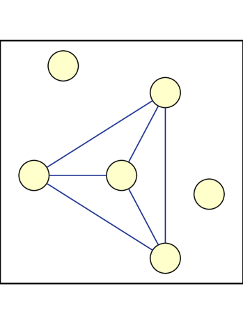
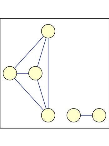
Another simple exponential random graph model is given by (49). By the same reasoning as above $c_{\includegraphics[height=3.01389pt]{3.pdf}}$ and $c_{\includegraphics[height=3.01389pt]{9.pdf}}$ should have opposite signs in order to have non-trivial typical graphs. Fig. 3 shows again the region of admissible expectation values $p_{\includegraphics[height=3.01389pt]{9.pdf}}$ and $p_{\includegraphics[height=3.01389pt]{3.pdf}}$, all $6$-node graphs, and the line $p_{\includegraphics[height=3.01389pt]{3.pdf}}=p_{\includegraphics[height=3.01389pt]{9.pdf}}=p_{-}$ of the Erdős-Rényi graphs. The minimal energy graphs can be easily understood in this example. In the case of negative $c_{\includegraphics[height=3.01389pt]{9.pdf}}$ and positive $c_{\includegraphics[height=3.01389pt]{3.pdf}}$ triangles are preferred. The minimal energy graphs are lying on the lower boundary of the admissible region and are non-connected graphs with fully connected components that could be considered as the ideal case of a “community structure” (see for instance Newman2004 ). The size of the components depends on the concrete values of the parameters. If the components are of different size, the graph is fully assortative, i.e. $r=1$. In the opposite case of positive $c_{\includegraphics[height=3.01389pt]{9.pdf}}$ and negative $c_{\includegraphics[height=3.01389pt]{3.pdf}}$ triangles are suppressed, and the minimal energy graph is a complete bipartite graph. The numbers of nodes in the two subsets are equal if the total number of nodes is even. Fig. 3A shows this graph in the case of $6$ nodes. If the total number of nodes is odd, the numbers of nodes in the two subsets will differ by one. As a consequence the minimal energy graph in this case will be fully disassortative. This disassortativity is a consequence of the bipartiteness and the different size of the components, thus not very informative on its own. The same applies for the observed assortativity in the first case that is also the consequence of the very specific structure of these minimal energy graphs. At the moment it is not clear to which extent it is possible and reasonable to explain assortativity and disassortativity by a catalog of paradigmatic structures that correspond to minimal energy graphs in exponential random graphs model as in these simple examples.

5 Discussion

We have presented a formalism that allows to study and quantify systematically the structures of networks as statistical dependencies. In particular, we showed how popular measures of network structures such as the degree distribution, the cluster coefficient and the assortativity coefficient could be expressed by subgraph probabilities. This allows to situate graph ensembles with predetermined values of these properties in the elements of the hierarchy of exponential families (1) which illuminates both their relationship and to which extent they specify redundant information about the graph structure. Very often only a single property is studied. For instance in Newman2002 , a random graph model with given degree distribution and additionally given joint remaining degree distribution for connected links is considered. This model allows for control of the degree of assortativity, corresponding to a variation of $P(G)$ in one direction. Depending on the exponential family $\mathcal{E}_{k}$ chosen, there are many other directions with non-vanishing assortativity. Thus it remains unclear how relevant this particular direction is.

By identifying the subgraph counts as sufficient statistics for exponential random graph models we also provide a link to systematically incorporate motif analysis in the analysis of network structures. A more detailed analysis of this aspect is beyond the scope of this paper and will be presented elsewhere.

Appendix A Expressing the assortativity coefficient by subgraph counts

Due to the homogeneity assumption all expectation values occurring in (36) can be estimated as the average over all links in a given graph. Then the following relations to the subgraph counts are derived:

• $\langle d^{r,i}\rangle$:

  $$\widehat{\langle d^{r,i}\rangle} = \frac{\sum_{i,j}a_{ij}d^{r,i}_{ij}}{\sum_{i,j}a_{ij}}$$

  $$= \frac{\sum_{i,j}\left(a_{ij}\sum_{k\neq i,j}a_{ki}\right)}{\sum_{i,j}a_{ij}}$$

  $$= \frac{\sum_{i,j\neq k}a_{ki}a_{ij}}{\sum_{i,j}a_{ij}}$$

  $$= \frac{2\cdot n_{\includegraphics[height=3.01389pt]{2.pdf}}}{2\cdot n_{-}}=\frac{n_{\includegraphics[height=3.01389pt]{2.pdf}}}{n_{-}}$$

  Since the average is performed with respect to all links, nodes with high degree get high weights. Thus, even though $d^{r,i}_{ij}=d_{i}-1$, $\frac{1}{\sum_{i,j}a_{ij}}\sum_{i,j}d^{r,i}$ is not equal to $\frac{1}{N}\sum_{i}d_{i}-1$!

• $\langle d^{r,i}d^{r,j}\rangle$:

  $$\widehat{\langle d^{r,i}d^{r,j}\rangle} = \frac{\sum_{i,j}a_{ij}d^{r,i}_{ij}d^{r,j}_{ij}}{\sum_{i,j}a_{i}j}$$

  $$= \frac{\sum_{i,j}\left(a_{ij}\sum_{k\neq i,j}a_{ki}\sum_{l\neq i,j}a_{jl}\right)}{\sum_{i,j}a_{i}j}$$

  $$= \frac{\sum_{i,j\neq k}a_{ki}a_{ij}a_{jk}+\sum_{i,j\neq k\neq l}a_{ki}a_{ij}a_{jl}}{\sum_{i,j}a_{i}j}$$

  $$= \frac{3\cdot n_{\includegraphics[height=3.01389pt]{9.pdf}}+n_{\includegraphics[height=3.01389pt]{3.pdf}}}{n_{-}}$$

• $\langle(d^{r,i})^{2}\rangle$:

  $$\widehat{\langle(d^{r,i})^{2}\rangle} = \frac{\sum_{i,j}a_{ij}\left(\sum_{k\neq i,j}a_{ki}\right)^{2}}{\sum_{i,j}a_{ij}}$$

  $$= \frac{\sum_{i,j}\left(a_{ij}\sum_{k\neq i,j}a_{ki}\sum_{k^{\prime}\neq i,j}a_{k^{\prime}i}\right)}{\sum_{i,j}a_{ij}}$$

  $$= \frac{\sum_{i,j\neq k}a_{ij}\overbrace{a_{ki}^{2}}^{=a_{ki}}+\sum_{i,j\neq k\neq k^{\prime}}a_{ij}a_{ki}a_{k^{\prime}i}}{\sum_{i,j}a_{ij}}$$

  $$= \frac{2\cdot n_{\includegraphics[height=3.01389pt]{2.pdf}}+6\cdot n_{\includegraphics[height=3.01389pt]{4.pdf}}}{2\cdot n_{-}}$$

  $$= \frac{n_{\includegraphics[height=3.01389pt]{2.pdf}}+3n_{\includegraphics[height=3.01389pt]{4.pdf}}}{n_{-}}$$

Hence the assortativity expressed in subgraph counts is

$$\widehat{r^{2}} = \frac{3\cdot n_{\includegraphics[height=3.01389pt]{9.pdf}}+n_{\includegraphics[height=3.01389pt]{3.pdf}}-\frac{n_{\includegraphics[height=2.15277pt]{2.pdf}}^{2}}{n_{-}}}{\left(n_{\includegraphics[height=3.01389pt]{2.pdf}}+3\cdot n_{\includegraphics[height=3.01389pt]{4.pdf}}-\frac{n_{\includegraphics[height=2.15277pt]{2.pdf}}^{2}}{n_{-}}\right)}$$

$$= \frac{n_{-}\left(3\cdot n_{\includegraphics[height=3.01389pt]{9.pdf}}+n_{\includegraphics[height=3.01389pt]{3.pdf}}\right)-n_{\includegraphics[height=3.01389pt]{2.pdf}}^{2}}{\left(n_{-}n_{\includegraphics[height=3.01389pt]{2.pdf}}+3n_{-}n_{\includegraphics[height=3.01389pt]{4.pdf}}-n_{\includegraphics[height=3.01389pt]{2.pdf}}^{2}\right)}$$

$$= \frac{\frac{n_{-}}{n_{\includegraphics[height=2.15277pt]{2.pdf}}}\left(\frac{3n_{\includegraphics[height=2.15277pt]{9.pdf}}}{n_{\includegraphics[height=2.15277pt]{2.pdf}}}+\frac{n_{\includegraphics[height=2.15277pt]{3.pdf}}}{n_{\includegraphics[height=2.15277pt]{2.pdf}}}\right)-1}{\frac{n_{-}}{n_{\includegraphics[height=2.15277pt]{2.pdf}}}\left(\frac{3n_{\includegraphics[height=2.15277pt]{4.pdf}}}{n_{\includegraphics[height=2.15277pt]{2.pdf}}}+1\right)-1}\;.$$

References

• (1) Amari, S.I.: Information geometry on hierarchy of probability distributions. Information Theory, IEEE Transactions on 47(5), 1701–1711 (2001). DOI 10.1109/18.930911
• (2) Ay, N., Knauf, A.: Maximizing multi-information. Kybernetika 42, 517–538 (2006)
• (3) Ay, N., Olbrich, E., Bertschinger, N., Jost, J.: A unifying framework for complexity measures of finite systems. Working Paper 06-08-028, Santa Fe Institute (2006). Proceedings of ECCS’06.
• (4) Börner, K., Sanyal, S., Vespignani, A.: Network science. Annual Review of Information Science and Technology 41(1), 537–607 (2007). URL http://dx.doi.org/10.1002/aris.2007.1440410119
• (5) Deming, W., Stephan, F.: On least square adjustment of sampled frequency tables when the expected marginal totals are known. Annals of Mathematical Statistics 6, 427–444 (1940)
• (6) Frank, O., Strauss, D.: Markov graphs. Journal of the American Statistical Association 81(395), 832–842 (Sep., 1986). URL http://www.jstor.org/stable/2289017
• (7) Handcock, M.S.: Assessing degeneracy in statistical models of social networks. Tech. rep., CSSS (2003). Working Paper no. 39
• (8) Kahle, T., Olbrich, E., Jost, J., Ay, N.: Complexity measures from interaction structures. Phys. Rev. E 79, 026,201 (2009). URL http://arxiv.org/pdf/0806.2552v2
• (9) Newman, M.: Detecting community structure in networks. The European Physical Journal B - Condensed Matter and Complex Systems 38(2), 321–330 (2004). URL http://dx.doi.org/10.1140/epjb/e2004-00124-y
• (10) Newman, M.E.J.: Assortative mixing in networks. Phys. Rev. Lett. 89(20), 208,701 (2002). DOI 10.1103/PhysRevLett.89.208701. URL http://link.aps.org/doi/10.1103/PhysRevLett.89.208701
• (11) Robins, G., Pattison, P., Kalish, Y., Lusher, D.: An introduction to exponential random graph (p*) models for social networks. Social Networks 29(2), 173–191 (2007). URL http://www.sciencedirect.com/science/article/B6VD1-4M4CVKM-1/2/df27f691fa8b1fcfc94380da74bbab77
• (12) Steiner, L., Kahle, T.: cipi—computing information projections iterativly. Available at http://personal-homepages.mis.mpg.de/kahle/cipi
• (13) Winkler, G.: Image Analysis, Random Fields and Markov Chain Monte Carlo Methods, 2nd edn. Springer (2003)