Statistical Laws in Urban Mobility from microscopic GPS data in the area of Florence

Abstract

The application of Statistical Physics to social systems is mainly related to the search for macroscopic laws, that can be derived from experimental data averaged in time or space,assuming the system in a steady state. One of the major goals would be to find a connection between the statistical laws to the microscopic properties: for example to understand the nature of the microscopic interactions or to point out the existence of interaction networks. The probability theory suggests the existence of few classes of stationary distributions in the thermodynamics limit, so that the question is if a statistical physics approach could be able to enroll the complex nature of the social systems. We have analyzed a large GPS data base for single vehicle mobility in the Florence urban area, obtaining statistical laws for path lengths, for activity downtimes and for activity degrees. We show also that simple generic assumptions on the microscopic behavior could explain the existence of stationary macroscopic laws, with an universal function describing the distribution. Our conclusion is that understanding the system complexity requires dynamical data-base for the microscopic evolution, that allow to solve both small space and time scales in order to study the transients.

, , ,
and

1 Introduction

Any statistical analysis of real systems is based on the Ergodic Principle for the microscopic dynamics, that implies the relaxation towards steady states and the independence property of elementary components. Even if the existence of microscopic interactions is necessary for the system to evolve toward a statistical equilibrium, in this state any particle moves independently from the others and all the particles are statistically equivalent (any particle may be representative for the whole). The thermodynamics laws that are derived from a statistical mechanics approach, concern some macroscopic observables of the system, evolving adiabatically with respect the microscopic relaxation time (i.e. we can consider the whole system in a almost equilibrium state), so that the effects of single particle dynamics are conveniently described by means of stochastic processes. As a consequence, there should exist a natural separation among macroscopic and microscopic space-time scales. Indeed space and time scales are expected to be strictly correlated: to understand small scale phenomena we need to solve short time scales and viceversa. Nevertheless the statistical mechanics has a great success in describing evolution of macroscopic systems and there is a strong effort to generalize the results for a non-equilibrium thermodynamics and for application to complex systems[1]. The statistical properties of social systems have been recently considered under a different point of view due to the possibility of recording large microscopic data sets[2, 3]. The main problem is what are the macroscopic effects of cognitive behavior for ”social particles”. Indeed the cognitive behavior would imply the existence of strong bidirectional interactions among the dynamics at different space and time scales of the system[4]. Emergence and self-organization characterize the macroscopic states, but the question is which macroscopic observables (if they exist) may enrol the complex nature of the system. These variables may also play an important role in the study of phase transitions and in the control parameters definition.

In Italy GPS data on individual vehicle paths are currently recorded for insurance reasons over a sample $\simeq 2\%$ of the whole private vehicle population[5, 6]. This data set gives the opportunity to study the individual mobility demand in urban contexts. The GPS data set contains the geographical coordinates, the time, the instantaneous velocity and the path length of individual trajectories at positions whose relative distance is of order $1\div 2$ km. Special signals are recorded when the engine is switched on and off. We remark that the data refer mainly to the private transportation mobility and that, due to privacy legal problems, we do not have any knowledge on the social features of individuals in the sample.

In this paper we analyze the statistical distributions of the path lengths of individual trajectories, of the activity downtime and the distribution of the monthly activity degree. Our aim is to point out the main macroscopic features of urban mobility studying their correlation with the idea of ”asystematic mobility” recently proposed by sociologists to explain the observational data in modern metropolis. We consider GPS data recorded during March 2008 in the Florence urban area. We show that some simple assumptions on single particles, like the existence of an ”individual mobility energy” and of an ”individual mobility time” that define the daily agenda, may explain the statistical laws emerging from the GPS data. Moreover in the equilibrium state individuals seem to minimize their interactions, behaving independently, so that the Maximum Entropy Principle of statistical mechanics can be applied[7]. These results are consistent with the idea that the sprawling phenomenon of modern cities implies that citizens move as stochastic particles[8]. Finally our analysis enlightens some average cognitive properties of individuals in urban mobility. The paper is organized as follows: in the first section we shortly described the GPS data base for vehicle mobility; in the remaining sections we discuss the three statistical laws on path lengths distribution, on the activities downtime and on the activity degree that are inferred from the data.

2 GPS data for vehicle mobility

A sample of $\simeq 2\%$ of the private vehicles in Italy has a GPS system for insurance reason. Any vehicle is associated to an ID number, so that it is possible to follow its mobility during a long time. Each datum gives position, velocity, covered distance from the previous measure and quality of signal. The data give a sampling of individual trajectories each $\simeq 2$ km, but a signal is also recorded any time the engine is switched on or off. The data suffer from the GPS limited precision, in particular when the GPS looses the satellite signal. These problems are especially relevant at starting points of the trajectories or when vehicles are parked inside a building, and short paths could be strongly affected by these pathologies. When the quality of signal is good the time precision of the recorded data is practically perfect, whereas the space precision is of the order of $10\,m$, usually sufficient to localize a vehicle on the road. Both the instantaneous velocity and the covered space, are given with an adequate precision since they result from a calculation based on GPS data recorded each second, but not registered. We have developed several methods to clean the data from spurious effects in order to avoid passible bias in the sample.

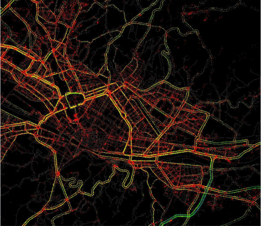
In the present work we consider the GPS data in the Florence urban area recorded during March 2008: these data are related to 35,000 vehicles in a circular area of radius $\simeq 30$ Km, around the historical center and defining $\simeq 2.5\times 10^{6}$ different trajectories. We have restricted our analysis to the trajectories which start inside a circle of 10 Km around the historical town and remain inside the considered area, so that with a good probability we select people living and moving in Florence. Then we look for the vehicles which perform daily loops from starting points that we identify as ”home”: in this case the number of trajectories reduces to $\simeq 4.\times 10^{5}$. In figure 1 we show the considered area where we have plotted the aggregate position GPS data: the color refers to the different instantaneous velocities (red means less than $30$ Km/h, whereas yellow refers to a velocity in the interval $30\div 60$ Km/h and the green to a velocity $\geq 60$ km/h).

Figure 1: Aggregated GPS position data in the Florence area recorded during March 2008; the red dots corresponds to a recorded instantaneous velocity $\leq 30$ Km/h, whereas the yellow dots correspond to velocities in the interval $30\div 60$ Km/h and the green dots to a velocity $\geq 60$ km/h.

We are completely ignorant on the social composition of the sample and on the specific drivers, but we expect that such individuals perform a mobility related to the activities present in the Florence area and have a certain knowledge of the road network.

3 Path length distribution

The activity sprawling that characterizes the modern metropolis has certainly a strong influence on the individual mobility demand[9]. Even if the Florence historical center is a very special area full of artistic and tourist attractions, but forbidden to private traffic, nevertheless we assume the activities randomly distributed in the urban system. This hypothesis is quite reasonable because we consider a large urban area and our sample is surely composed by inhabitants and not tourists. As a consequence, we expect that the citizen mobility agenda are influenced by individual features rather than by the city structure. In cities the stationary average traffic state should emerge as the result of individual interactions of cognitive particles which share the same spatial resources. In particular we assume that drivers organize their mobility, by applying a minimization strategy of the interactions with other individuals[10]. In this conceptual framework, the mobility can be seen as the realization of many independent individual agenda and the dynamical properties become similar to that of a Boltzmann gas. Even if it is obviously true that individuals are non-identical particles, path length and activity downtime can be considered common mobility features to all people, and good candidates for a statistical physics approach to describe the stationary state. For each vehicle we have recorded the total lengths $L$ of his daily round trips for the whole considered period. The length distribution is plotted in fig. 2 where we point out the existence of an interpolation with a Maxwell-Boltzmann distribution

$$p(L)=L_{0}\exp(-L/L_{0})$$ (1)

with $L_{0}\simeq 25$ Km the characteristic daily path length.

Figure 2: Empirical distribution of the daily mobility length $L$(dots). The continuous line is an interpolation with a Maxwell-Boltzmann distribution with average value $<L>\simeq 25\,Km$.

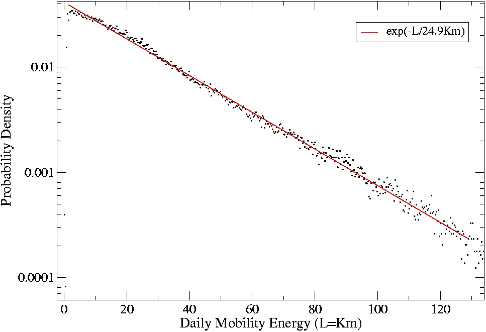
The distribution (1) provides a very good fit of the experimental data, and it can be justified by the Maximum Entropy Principle under the assumption that the individuals are independent particles and that there exists an average daily trip length in the population (see supplementary material). In such a case the distribution (1) is realized when any particle chooses its mobility energy randomly. It is straightforward to associate an individual ”mobility energy” to the daily path lengths. The assumption that citizens organize their mobility as they own an internal ”mobility energy”, agrees with similar hypotheses discussed by R.Kolb and D.Helbing[11] to explain the daily travel-time distributions for different transport modes.

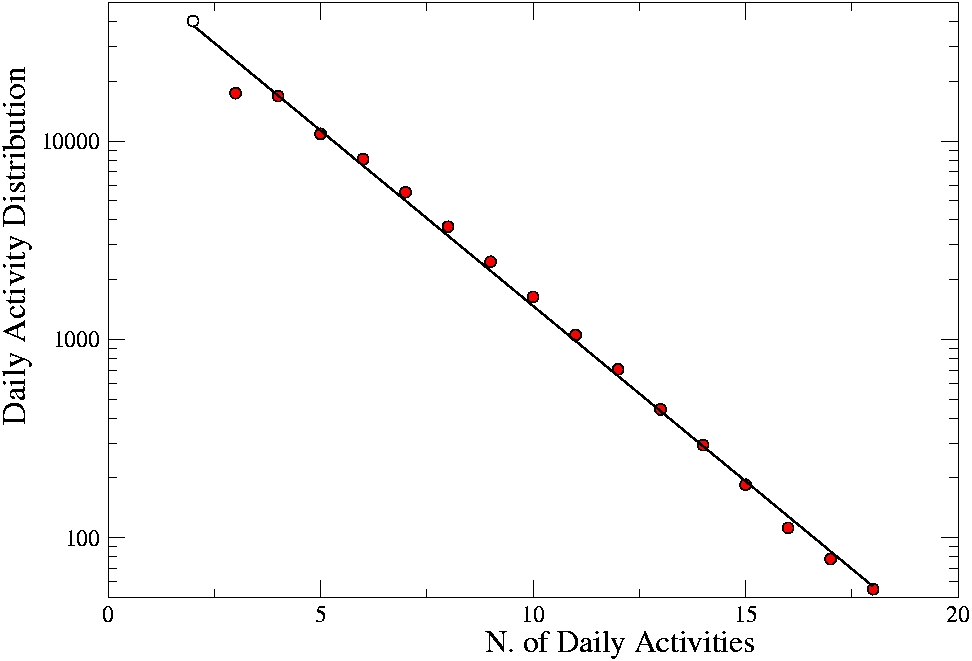
In order to investigate the concept of the mobility energy together with the Maximum Entropy Principle, we consider the relation between the daily path length and the single trip path length, building up the rank distribution of individual daily activities. To define an activity from GPS mobility data, we apply a clustering procedure to vehicle stop positions, identifying the positions which lie in a circle of diameter $\simeq 500$ m (this is considered a acceptable distance between the true destination and the parking place[12]). Moreover we have associated an activity when the elapsed time before the next trip is greater than 15 minutes. In figure 3 we plot the rank distribution for the daily activities together with an exponential interpolation

$$p(k)\propto a^{k}$$ (2)

that provides a very good fit of experimental observations. The equation (2) is consistent with the assumption that, in average, the individuals behave as independent random particles which define their daily agenda in a random way.

Figure 3: Rank distribution of daily activities computed from the GPS data(circles). The continuous line is an exponential interpolation according to (2) with $a\simeq.7$.

According to previous hypotheses, it is possible to compute in analytical way the single trip length distribution, as the distribution realized by uniformly spreading $k$ points into a given segment of length $L$. A simple calculation provides the single trip length distribution in the form (see appendix)

$$p_{N}(x)={c\over L}\sum_{k=1}^{N}(k+1)ka^{k}(1-x/L)^{k-1}$$ (3)

where $c$ is a normalizing factor and $N$ is the maximum number of daily activities; we remark that the choice of the points in the segment is contextual without any time-ordering. It is quite natural to assume that there should exist a correlation between the number of daily activities $N$ and the daily mobility length $L$, but the GPS data do not suggest any correlation function, so that we decided to use an effective daily length in the theoretical distribution (3) to make a comparison with the empirical one. It turns out that If we exclude the very short paths, the curve (3) fits very well with the experimental data (see fig. 4) with an effective daily mobility length $L=30$ Km (the result is not too sensitive to this particular value and we have not performed any optimization procedure).

Figure 4: Single trip length distribution computed from the GPS data(circles). The continuous line corresponds to an interpolation with the distribution (3) by fixing the maximal number of daily activities at $N=18$ according to fig. 3 and an effective daily mobility length $L=30$ Km (not optimized).

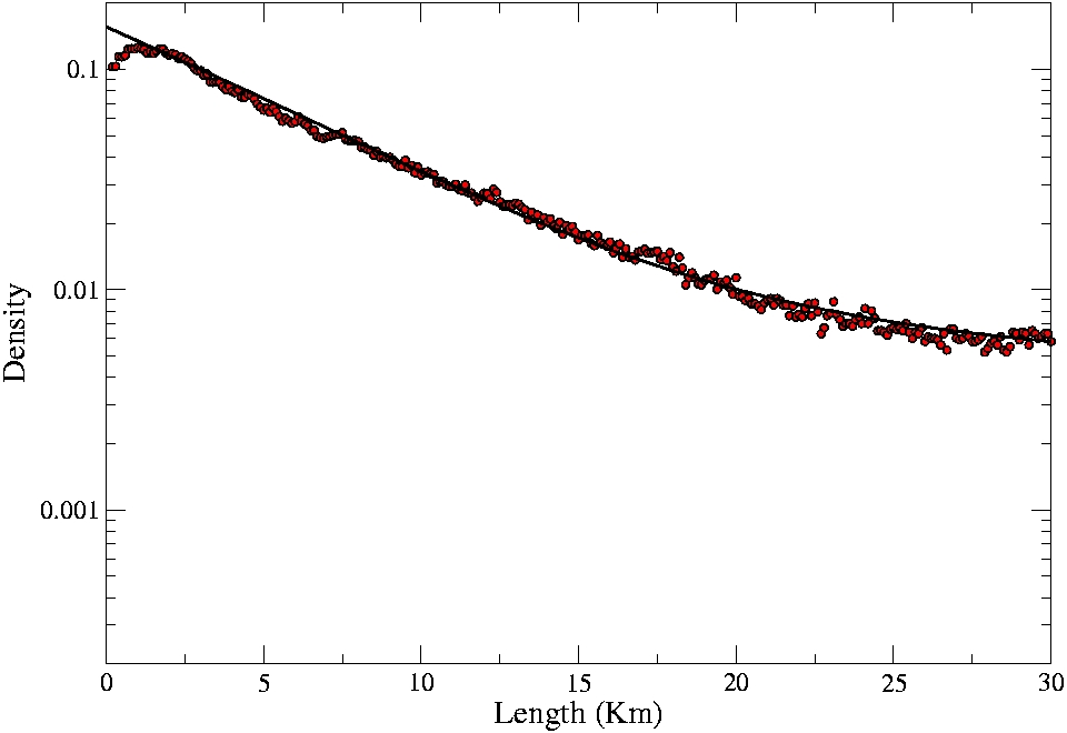
As a final remark from the figure 4, we observe that the long trip length distribution differs from an exponential behavior and it rather seems to follow a power law.

4 Activity downtime distribution

Time is the second fundamental individual variable of human mobility, directly related to the dynamical realization of daily agenda. From the GPS data base in the Florence area we have computed the downtime spent in each daily activity by a fixed individual; we discard from the activities the sleeping time linked to circadian rhythms. The distribution of the activity downtimes of the recorded individuals is plotted in fig. 5, recovering the well known Benford’s law[13].

Figure 5: Activity downtime distribution computed from the GPS data(circles); we have normalized the data at the maximal value. The continuous line corresponds to an interpolation with a power law $x^{\alpha}$ with $\alpha=.97$ which is consistent with the Benford’s law (4).

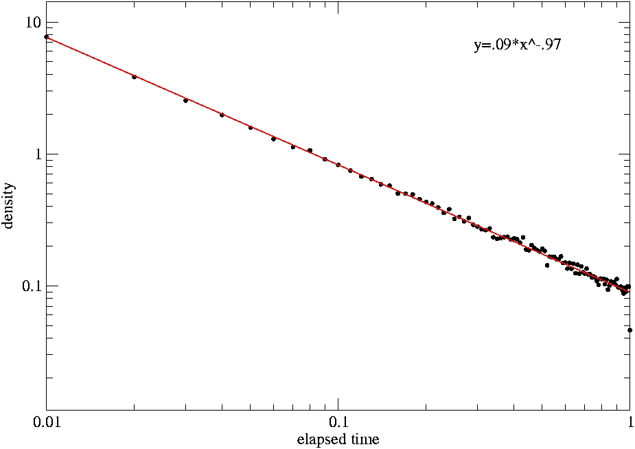
In order to give a microscopical interpretation of the empirical downtime distribution, we assume that individuals cannot determine a priori each activity downtime, because this is varied depending on unpredictable circumstances. According to this hypothesis, in the average, each particle has a finite mobility time at disposal to perform the desired activities, and he consumes the time in successive random choices up to the end of the whole mobility time. If one computes the interval distribution that is obtained by choosing successively $k$ points in a given segment, one get analytically the Benford’s distribution[13]

$$p(t)\propto-\sum_{k=1}^{N}{(\ln t)^{(}k-1)\over(k-1)!}\simeq{1\over t}$$ (4)

Shortly, the statistical results of the monthly mobility in the Florence area, recorded by the GPS data on vehicles, suggest that the macroscopic average properties are the same of those of Boltzmann’s particles moving in a homogeneous space with an average energy and a finite time at disposal. The energy introduces a global constraint in the individual daily mobility, whereas the time can be seen as a local constraint in the activity planning since it is consumed step by step.

However computing the distribution of the total activity downtime for the monitored vehicles, we can get an idea of the typology of urban mobility described by our sample.

Figure 6: Daily activity downtime distribution. We remark three characters of the underlying mobility: the first peak is related to short downtime activities ($\simeq 1$ h), the second peak ($\simeq$ 10 h) is probably due to working people and the long tail ($\geq 12$ h) could be explained by the presence of business vehicles that are used by different people.

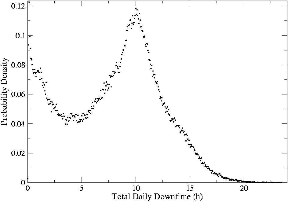
The results are plotted in fig. 6 We remark the presence of two peaks: one is related to short downtime activities, that probably corresponds to a specific use of the vehicle for a single trip, whereas the second peak centered at $\simeq 10$ h denotes people performing a more complex mobility agenda, which contains the working activities. Finally the presence of a long queue for the daily activity downtime ($\geq 12$ h) is probably due to business vehicles in our sample, that are used by different people.

5 Activity degree distribution

Both the Boltzmann distribution for the mobility energy and the Benford’s law for the activity downtime enroll stochastic features of the system, but they do not explain how such features can be related to the individual daily agenda, that are certainly the result of a cognitive behavior. In order to study this question, we perform a statistical analysis of the downtime related to daily activities, considering the monthly degree $k$ for the different individual activities (i.e. the number of times that a citizen repeats a certain activity during a month)[14]. Let $t$ the activity downtime, we introduce the join probability $p(t,k)$ to denote the probability of finding a $k$-degree activity associated to a downtime $t$. Then by definition we have to recover the Benford’s law (4) by summing over $k$

$$\sum_{k}p(t,k)\propto{1\over t}$$ (5)

We have also the equality

$$p(t,k)=p(t\mid k)kp(k)$$

where $p(t\mid k)$ is the conditional probability for a downtime $t$ considering only the $k$-degree activities, and $p(k)$ is the probability to detect a $k$ degree activity; the factor $k$ takes into account the multiplicity of the $k$ degree activities. The study of the conditional probability $p(t\mid k)$ can shed some light to understand the mobility habits related to the use of private vehicles and to face the question of the relevance of repeated activities both in the mobility and in the use of time. Remarkably the experimental observation suggest the existence of an universal probability distribution $f(u)$ for the normalized downtime $t/<t>_{k}$:

$$p(t\mid k)={f(t/<t>_{k})\over<t>_{k}}$$ (6)

where $<t>_{k}$ is the average downtime for the $k$-degree activities. We read this universal function as the signature of the fact that individuals organize their time, when performing a private car mobility, in a common way independently from the specific activity, i.e. the relative downtime fluctuations are the result of a stochastic universal mechanism. Moreover there should exist a common feature among the individuals, concerning how they manage the downtime related to the $k$-degree activities, since only the average value $<t>_{k}$ characterizes the $k$ dependence of the conditional probability $p(t\mid k)$. This universal character could be explained thinking that the $t/<t>_{k}$ variable is a generic ”measure” of the mobility actions, valid for every individual. More precisely $t/<t>_{k}$ can be considered the temporal norm for all the mobility related activities. From the empirical data we detect $\simeq 3\times 10^{5}$ activity downtimes and we have computed the dependence of the average value $<t>_{k}$ using the degree $k=3,..,20$.

Figure 7: Dependence of the average downtime $<t>_{k}$ from the activities degree $k$. The continuous line refer to a possible interpolation with the exponential function (7).

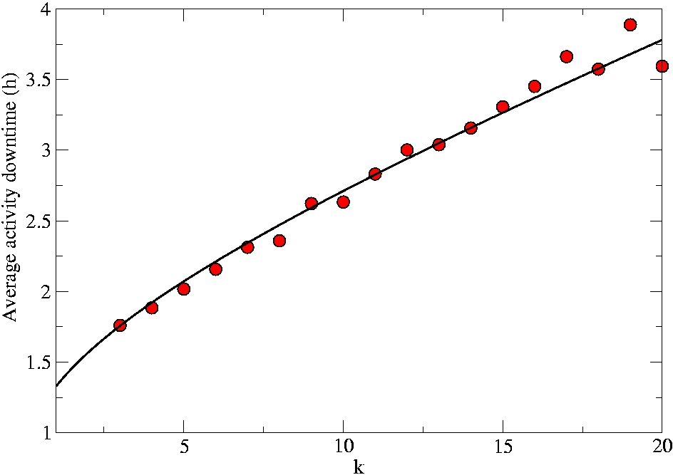
It is evident from fig. 7 that we have an almost linearly increasing behavior of $<t>_{k}$ as the degree $k$ increases. This means the existence of a relation between the activity degree and the activity ”use value” (individual satisfaction, profit, etc…) that introduces an individual tendency to repeat and to spend time in the activities with a relevant added value[15]. A possible local interpolation of the empirical data is obtained by using the function (continuous line in fig. 7)

$$<t>_{k}\propto\exp(\gamma k^{a})$$ (7)

where $a\simeq.3$ and $\gamma\simeq.7$. In figures 8,9 and 10 we plot the empirical probability densities for different degree (from $k=3$ to $k=20$) to investigate the existence of the universal distribution $f(u)$.

Figure 8: Empirical distributions of the $k$-degree activity downtime as a function of the normalized downtime $t/<t>_{k}$. The different symbols refer to the different activity degrees: $k=3$ (circles), $k=4$ (squares), $k=5$ (rhumbs), $k=6$ (up triangles), $k=7$ (down triangles).

Figure 9: Empirical distributions of the $k$-degree activity downtime as a function of the normalized downtime $t/<t>_{k}$. The different symbols refer to the different activity degrees: $k=8$ (circles), $k=9$ (squares), $k=10$ (rhumbs), $k=11$ (up triangles), $k=12$ (down triangles)..

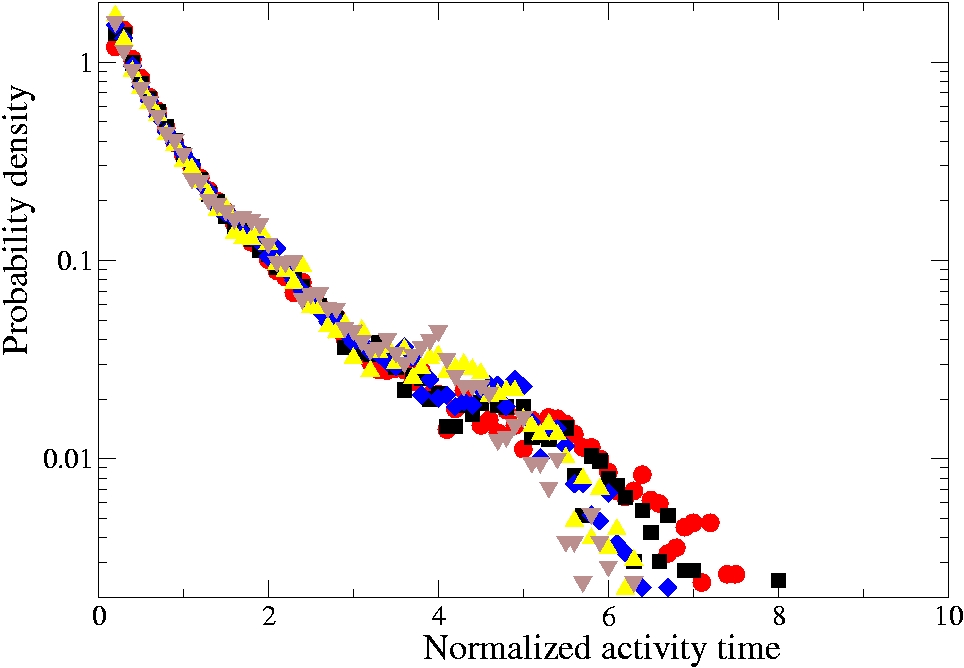
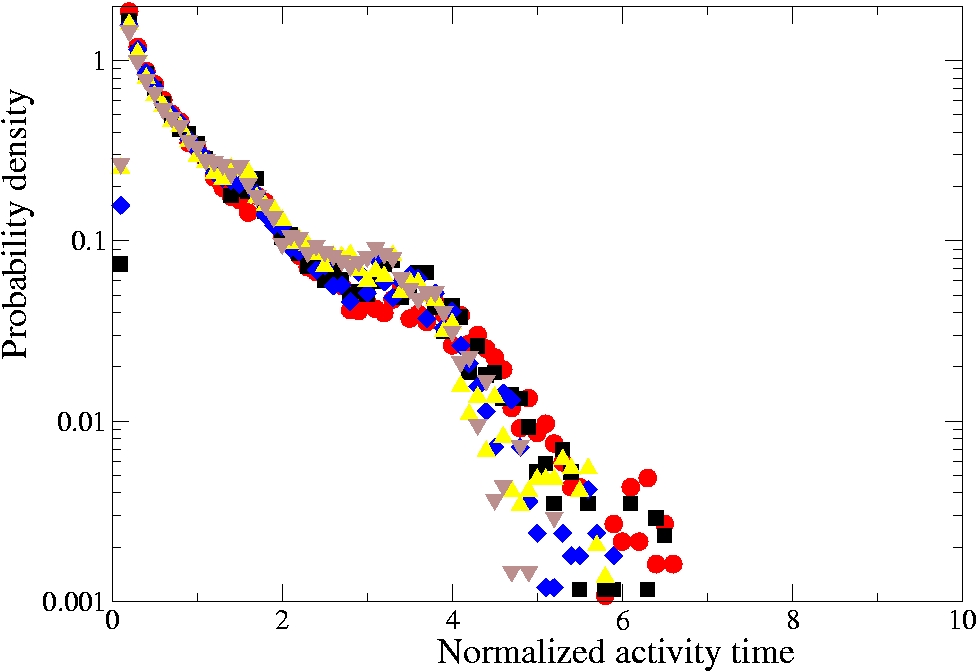
There is a decreasing of the data number as $k$ increases, but all the distributions are computed with a sample of the same order (from $4\times 10^{4}$ to $10^{4}$). The figures enlighten three different features. There is a collapse of all the curves on a unique distribution: this is clear in the figure 8 (the tail spread is consistent with statistical fluctuations) and in the first part of all the plotted distributions that contains the great majority of the data. All the distributions show a big contribution from the short times activities and a fast decaying tail for large $(t/<t_{k}>)>2$.

Figure 10: Empirical distributions of the $k$-degree activity downtime as a function of the normalized downtime $t/<t>_{k}$. The different symbols refer to the different activity degrees: $k=16$ (circles), $k=17$ (squares), $k=18$ (rhumbs), $k=19$ (up triangles), $k=20$ (down triangles).

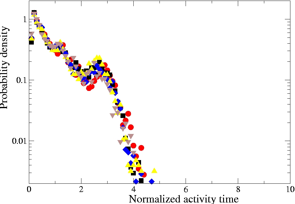
There is a smooth rise of a ”signal” as $k$ increases denoted by the appearance of two peaks at $t/<t>_{k}\simeq 1,3$: this is clear in the last figure 10. Therefore the empirical observation gives a strong indication for the existence of an universal distribution $f(u)$ for the normalized activity downtime, even if when we consider high degree activities ($k\geq 10$) some new features appear but with a small statistical weight. A possible interpolation of the distribution $f(u)$ is given by

$$f(u)\propto{1\over u}e^{-\alpha u}$$ (8)

where the coefficient $\alpha$ has a value $\simeq.4$. The distribution (8) is singular at the origin so that the interpolation is certainly approximated at $u\to 0$ (see fig. 14 in the appendix).

Figure 11: Ratio between the empirical distributions of the $k$-degree activity downtime and the interpolation (7) as a function of time (h). The different symbols refer to the different activity degrees: $k=16$ (circles), $k=17$ (squares), $k=18$ (rhumbs), $k=19$ (up triangles), $k=20$ (down triangles). Two peaks at a downtime $t\simeq 4$ h and at $t\simeq 10$ h that are common to all the distributions can be observed.

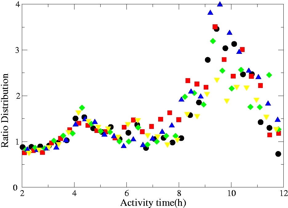
The exponential decay is the typical Boltzmann statistics as for the path length distribution, whereas the $u^{-1}$ behavior is consistent with the Benford’s law for the downtime distribution. So that this ”universal distribution” seems to mix both the features shown in fig. 4 and 5. To explain the singular $f(u)$ trend at the origin, we guess that it can be a sign of a strong free-will in the individual behavior in the short time activity range. Surely for a more precise justification further study are required. We can use the interpolation (8) to extract the signal from the high degree activity distribution, by computing the ratio between the empirical distribution data and the interpolation (7); in the figure 11 we plot the ratio distribution results. As it can be seen, the empirical data define two peaks centered at $t\simeq 4$ hours and at $t\simeq 10$ that are common to all the distributions when $k=16,...,20$. Even if these peaks are not statistically relevant, they can be related to individuals that perform repeated activities linked to the canonical working time schedule. Clearly the working time schedule introduces further constrains to the individual mobility agenda, that are not taken into account by the universal distribution $f(u)$. Now the existence of an universal distribution implies (cfr. eq. (6))

$$p(t,k)=f\left({t\over<t>_{k}}\right){kp(k)\over<t_{k}>}$$ (9)

Then using the interpolation (7) and performing the change of variable $u(k)=t/\exp(\gamma k^{a})$, we obtain that the Benford’s law (5) implies a power law distribution for the activity degrees(see appendix)

$$p(k)\simeq{1\over k^{2-a}}$$ (10)

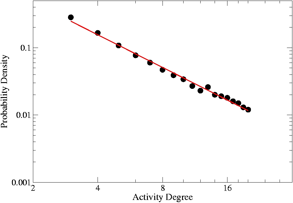
According to the estimate (7), we expect an exponent $\simeq-1.7$. In fig. 12 we plot the empirical activity degree distribution with a numerical interpolation by a power law $k^{-b}$; the data provide $b\simeq 1.6$ which is consistent with the analytical estimate (10).

Figure 12: Empirical distributions of the activity degree (circles). In a log-log scale we enlighten the interpolation with a power law $k^{-b}$ with $b\simeq 1.6$ (continuous curve).

6 Conclusions

The citizens mobility is an interesting social phenomenon that involves a large number of ”intelligent” elementary components with a free will individual property, so that we can speak of a cognitive dynamics. In this paper we analyze a lot of car mobility data for the Florence area, showing the emergence of three robust statistical laws for the path lengths, the activity downtime and degree. These laws can be explained as the direct consequence of some simple hypotheses as the particle independence, and above all assuming the existence of an individual mobility energy and of a finite individual time spent for the desired urban activities. Moreover, from the downtime distribution we deduce an universal function which fits with empirical observations and data. We think that this universal function can be interpreted as an indication of the cognitive time perception common to all human beings, or at least surely common to the car drivers. Finally the urban mobility is clearly complex, but the our steady state statistics cannot point out the typical complexity signatures as, for instance, self-organized states. To detect complexity in mobility dynamics, it is necessary to investigate the transients, i.e. the states far from equilibrium.

7 AKNOWLEDGEMENTS

We thank OCTO Telematics for the access to the GPS data base on the Florence area. The authors are in debt with Prof. Dirk Helbing and Prof. Luciano Pietronero for several stimulating discussions.

8 Appendix

Let us consider $k$ stochastic variables uniformly distributed in the unit segment, the probability that a segment of length $\leq x$ is empty can be estimated according

$${\cal P}(\leq x)=1-(1-x)^{k}$$

As a consequence the probability density that a certain segment $x$ is empty is given by

$$p(x)={d{\cal P}\over dx}=k(1-x)^{k-1}$$

Therefore if one choices randomly an integer number $k$ in the interval $[1,N]$, the probability density for a segment of length $x$ conditioned by the choice $k$ is

$$p_{k}(x)\propto(k+1)k(1-x)^{k-1}\qquad x\in[0,1]$$ (11)

since we have to take into account $k+1$ possible segments. The probability (11) has to be weighted by the probability $p(k)\propto a^{k}$ to have $k$ points so that the probability density to detect a segment of length $x$ for any choice $k$ is

$$p_{N}(x)={(1-a)^{2}\over(2-a)a(1-a^{N})-Na^{N+1}(1-a)}\sum_{k=1}^{N}(k+1)ka^{k}(1-x)^{n-1}$$ (12)

where we have introduced a normalizing factor. In fig. 13 we show the comparison between the equation (12) and a MonteCarlo distribution with $N=7$.

Figure 13: MonteCarlo simulations for the probability density of intervals in a given segment defined by randomly choosing $n$ points in the interval uniformly distributed with $n$ a random integer $\leq N=7$. The continuous line is the plot of the theoretical distribution (12).

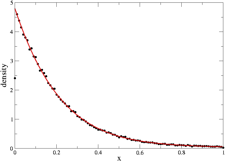
The distribution (12) allows an analytical approach to the single trip length distribution (cfr. fig. 4 in the paper).

The empirical conditional distributions $p(t\mid k)$ for different degrees $k$ as a function of the normalized activity downtime $t/<t>_{k}$ suggests that the statistically relevant can be described according to

$$p(t\mid k)={f(t/<t>_{k})\over<t>_{k}}$$ (13)

where we introduce an universal function $f(t/<t>_{k})$ which can be interpolated by

$$f(u)\propto{1\over u}e^{-\alpha u}$$ (14)

The results are shown in figure 14 for the activity degrees $k=3,..,20$.

Figure 14: Empirical distributions for the conditional probabilities $p(t\mid k)$ for activities degrees $k=3,..,20$ as a function of the normalized activity downtime $t/<t>_{k}$ (different symbols). The continuous line refers to an interpolation with the function (4).

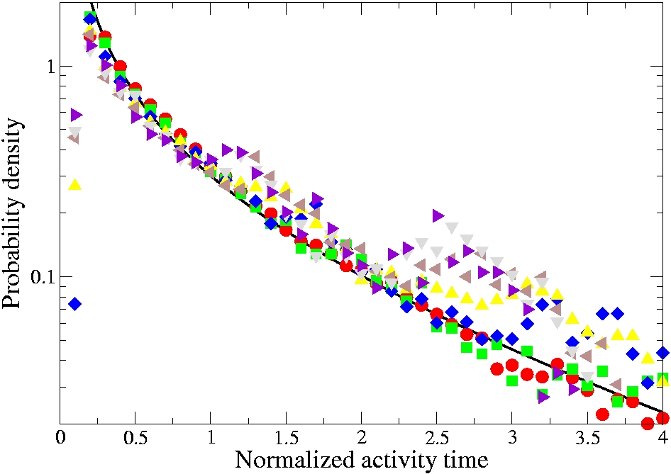
There is a strict relation between the activity degree distribution (see fig. 12 in the paper) and the existence of an universal distribution probability $f(u)$ in eq. (13) Indeed taking advantage from the dependence of $<t>_{k}$ on the degree $k$ pointed out by experimental observations (see fig. 7 in the paper) we perform the change of variables

$$\cases{t}&=t\\ u=t/<t>_{k}\\$$ (15)

in the join probability distribution $p(k,t)$ of degree and downtime (cfr. eq. (9)). Using the definition (5), we get the new distribution

$$p^{\prime}(u,t)=f(u)k(u)p(k(u)){dk\over du}=-f(u)kp(k){<t>_{k}\over t}\left({d<t>_{k}\over dk}\right)^{-1}$$

where $k$ has to be read $k(u)$ in the r.h.s. and $p(k)$ is the activity degree distribution. In the previous formula we approximate interpolate the discrete variable $k$ with a continuous variable. By integrating of $u$ we have to recover the Benford’s law $\propto 1/t$ for the global activity downtime distribution (see fig. 5 in the paper). Since $f(u)$ is normalized as probability distribution, this is possible if

$$kp(k)<t>_{k}\left({d<t>_{k}\over dk}\right)^{-1}={\rm const.}$$ (16)

According to the interpolation $<t>_{k}\propto\exp\gamma k^{a}$ of the experimental data as shown in the figure 7 in the paper, we explicitly have

$${d<t>_{k}\over dk}\propto k^{a-1}e^{\gamma k^{a}}\propto k^{a-1}<t>_{k}$$

therefore the condition (16) reads

$$k^{2-a}p(k)={\rm const.}$$

i.e. a power law distribution of the activity degree with exponent $\leq 2$. This is consistent with the experimental observations as shown by the figure 12 in the paper.

References

- [1] R. Balescu Equilibrium and nonequilibrium statistical mechanics, New York, Wiley-Interscience, (1975).
- [2] D. Brockmann, L. Hufnagel3 and T. Geisel The scaling laws of human travel Nature, 439, (2006), pp. 462-465.
- [3] M.C. González1, C.A. Hidalgo and A.L. Barabási Understanding individual human mobility patterns Nature, 453, (5 June 2008), pp 779-782.
- [4] T.van Gelder, The dynamical hypothesis in cognitive science, Behavioral and Brain Sciences 21, (1998), pp. 615-628.
- [5] http://traffico.octotelematics.it/.
- [6] A. Bazzani, S. Rambaldi, B. Giorgini and L. Giovannini Mobility in modern cities: looking for physical laws ECCS07 Conference Proceedings, n. 132, (2007).
- [7] L.D. Landau,E.M. Lifshitz Statistical Physics - Course of Theoretical Physics 5, Third edition, Butterworth-Heinemann, (1980)
- [8] M. Batty Cities and Complexity The MIT Press, Cambridge, Massachusetts (2005).
- [9] T. Domencich and D.L. McFadden Urban Travel Demand: A Behavioral Analysis North-Holland Publishing Co., (1975).
- [10] I. Volkov, J.R. Banavar, S.P. Hubbell and A. Maritan Infering species interactions in tropical forests PNAS, 106-33, (2009), pp. 13854-13859.
- [11] R. Kölb and D. Helbing Energy laws in human travel behaviour, New J. Phys. 5, (2003) pp.48.1-48.12.
- [12] I. Benenson, K. Martens From modeling parking search to establishing urban policy Kunstliche Intelligenz, 3, (2008), pp.3-8.
- [13] L. Pietronero, E. Tosatti, V. Tosatti and A. Vespignani, Explaining the uneven distribution of numbers in nature: The Laws of Benford and Zipf Physica A: Statistical Mechanics and its Applications, 293 (12), (2001), pp. 297-304.
- [14] S. Schönfelder and K.W. Axhausen Structure and innovation of human activity space Arbeitsbericht Verkerhrs und Raumplanung 258, IVT and ETH Zurich, (2004).
- [15] P. S. Samuelson and W. D. Nordhaus Economics 17th Edition, McGraw-Hill, (2004).
8 Appendix
Let us consider stochastic variables uniformly distributed in the unit segment, the probability that a segment of length is empty can be estimated according