Diffusion and Localization of Cold Atoms in 3D Optical Speckle

Abstract

In this work we re-formulate and solve the self-consistent theory for localization to a Bose-Einstein condensate expanding in a 3D optical speckle. The long-range nature of the fluctuations in the potential energy, treated in the self-consistent Born approximation, make the scattering strongly velocity dependent, and its consequences for mobility edge and fraction of localized atoms have been investigated numerically.

1 Introduction

Anderson localization is by now a phenomenon that has been widely investigated, both theoretically and experimentally, and for many different kinds of waves, from electrons, to electromagnetic waves, ultrasound pht1 , and cold atoms pht2 . To understand Anderson localization and to provide quantitative predictions for experiments, many tool models have been proposed, among which the Anderson model is undoubtedly the best known. This model describes a noninteracting and electron, tightly bound to the nucleus, but capable to tunnel to nearby atoms. Already in the celebrated 1958 paper pwa , Anderson demonstrated how this model highlights the role of dimensionality. A genuine mobility edge only occurs in dimensions larger than 2 kramer . For classical waves, a few observations on 3D localization have been reported died ; page .

The tight binding model is highly relevant to understand 3D dynamical localization of cold atoms dynamic . However, is not appropriate to describe localization of many other waves, where the starting point is much more a diffuse, extended motion, rather than a tightly bound state. Localization of electromagnetic waves in 3D disordered media for instance, is much more a diffusion problem than a problem of tunneling to nearest neighbors. The scaling theory of localization g4 , as well as the Thouless criterion thou , both deal with conductance, and thus use the diffuse motion as a starting point.

The self-consistent theory, first formulated by Vollhardt and Wölfle in 1981 for 2D electron conductivity vw , was the first work that explicitly calculated how quantum corrections affect the classical ”Drude” picture, to make way for localization. Despite its evident perturbational nature, the theory has been successful because it provides a microscopic picture of finite-size scaling, reproduces the Ioffe-Regel criterion for the mobility edge in 3D, and locates the mobility edge of the tight-binding model quite accurately kroha . The aim of the present work is to revisit and apply this theory to the localization of cold atoms in optical speckle.

The first experiments on 1D cold atom localization have been carried out recently coldatomloc . The atoms are released from a BEC and subsequently expand in a potential energy landscape created by optical speckle, supposed free of mutual interactions. Both theory 1Dquasi and experiment have revealed the presence of a quasi-mobility edge in 1D. Atoms with velocities $v>\hbar/m\xi$ ($\xi$ is the correlation length of the disorder) can hardly be scattered because this would imply a momentum transfer larger than $\hbar/\xi$ which the random speckle cannot support. As a result the localization length is infinite in the Born approximation, though finite and large when all orders are taken into account. This somewhat surprising result highlights the impact of long-range correlations in 1D. In higher dimensions, small angle scattering can still lead to small enough momentum transfer to be transferred to the speckle, even for large velocities, so that this quasi-mobility edge does not occur. Yet, correlations are expected to affect localization, since the potential field sensed by the atom strongly depends on its velocity, and strong forward scattering is not favorable for localization to occur. In addition, near the 3D mobility edge the disorder is necessarily large so that the spectral function of the atoms is not strongly peaked near energies $E={p^{2}}/{2m}$, neither has it a Lorentzian broadening.

2 Self-consistent Born Approximation

In the following we consider the scattering of a noninteracting atom with energy $E$ and momentum $\mathbf{p}$ from a disordered potential $V(\mathbf{r})$. Two properties are specific for an optical potential. Firstly, the fluctuations $\delta V(\mathbf{r})$ are determined by the optical intensity and not by the complex field. This means that they are not Gaussian but rather Poisonnian. As a result, the two-point correlation will in principle not be sufficient to describe the full scattering statistics. Secondly, the correlation function, given by $\langle\delta V(\mathbf{r})\delta V(\mathbf{r}^{\prime})\rangle=U\mathrm{sinc}^{2}(\Delta r/\xi)$, is long range. Here $U=\langle V\rangle^{2}$ depends on the average optical intensity. It is not difficult to see that the Born approximation breaks down at energies $E\preceq U/E_{\xi}$ kuhn , with $E_{\xi}=\hbar^{2}/2m\xi^{2}$ an important energy scale related to correlations. As usual we expect matter localization to occur at small energies, near the band edge of the spectrum. Another consequence of the long-range correlations is that scattering strongly depends on the De Broglie wave length and thus on the velocity of the atom. This makes it impossible to define a mean free path $\ell$ in the usual way, that is from the exponential decay of the ensemble-averaged Green function pr .

In the following we shall cope with the second problem. The ensemble-averaged Green function is written in terms of a complex self-energy as $G(E,k)=[E-p^{2}/2m-\Sigma(E,p)]^{-1}$ pr . We shall apply the Self-consistent Born Approximation (SCBA) according to which the complex self-energy $\Sigma(E,p)$ of the atom is calculated from scba

$$\Sigma(E,k)=\sum_{\mathbf{k}^{\prime}}\frac{U(\mathbf{k}-\mathbf{k}^{\prime})}{E-k^{\prime 2}-\Sigma(E,k^{\prime})}$$ (1)

In this equation, $\sum_{\mathbf{k}}\equiv\int\mathrm{d}^{3}\mathbf{k}/(2\pi)^{3}$, and from now, all energies, including $\Sigma(E,p)$, are expressed in units of the energy scale $E_{\xi}$. Momenta are expressed as $\mathbf{p}=\hbar\mathbf{k}$ with the De Broglie wave number $\mathbf{k}$ expressed in units of $1/\xi$. In Eq. (1), $U(\mathbf{k}-\mathbf{k}^{\prime})$ represents the structure function associated with the speckle correlation, which determines the angular profile in single scattering kuhn . The SCBA is convenient because its imaginary part expresses the generalized optical theorem in single scattering pr . In addition, it avoids the bound state at negative energies predicted by the first Born approximation. In Ref. anna the SCBA was solved analytically for cold atoms and zero-range correlations.

Equation (1) has been solved by iteration, with spline interpolation between 500 points $0<k_{n}<3$. The angular integral can be performed analytically. Typically 10-20 iterations have been necessary to ensure good convergence. In Figure 1 we show real and imaginary part of $\Sigma(E,k)$ for $U/E_{\xi}^{2}=1$ and $E=0$, and compare it to the first order Born approximation (FBA) applied in Ref. kuhn . As a realistic experimental reference we take ⁸⁷Ru-atoms released from a BEC with chemical potential $\mu=219\,h$ Hz into an optical speckle with correlation length $\xi=0,26$ $\mu$m. This reveals that $\mu$ and $E_{\xi}$ are equal energy scales in typical experiments. Equivalently, the De Broglie wavelength and the correlation length are competing length scales, $\lambda/2\pi\geq\xi$. To discriminate ”trivial trapping ” in deep random potential wells from ”genuine” Anderson localization, experimentalists wish to arrange the experiment such that the typical kinetic energies $\mu$ are somewhat larger than the typical fluctuations $\sqrt{U}$ in the potential energy coldatomloc . In that case, $U/E_{\xi}^{2}\geq 1$. We will comment on this choice later.

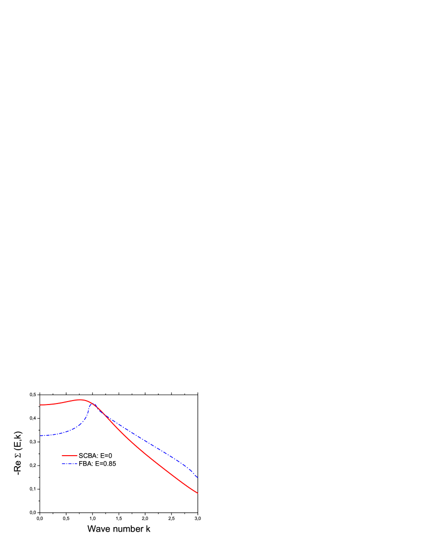
Figure 1: Imaginary (top) and real part (bottom) of the self energy (in units of $E_{\xi}$) of an atom in a speckle potential with $U/E_{\xi}^{2}=1$, as a function of wave number (in units of $1/\xi$) for an energy $E=0$, calculated in the self-consistent Born approximation (SCBA). The dashed line denotes the first Born approximation (FBA). To compensate for the shift in the band edge ($E_{b}/E_{\xi}=-0.85$) predicted by the SCBA, the FBA has been evaluated at $E/E_{\xi}=0.85$.

Figure 1 (top) shows $-\mathrm{Im}\,\Sigma(0,k)$ to be nonzero only for $k<3$. It is also seen that the FBA significantly overestimates the amount of scattering. The real part $\mathrm{Re}\,\Sigma(0,k)$ is clearly negative. This shifts the band edge of the energy spectrum to $E_{b}=-0.85$. The energy spectrum has a typical lower bound $-\sqrt{U}$, but the SCBA always locates the band edge at somewhat larger energies. The SCBA does probably not treat the (small) density of states near $E\approx-\sqrt{U}$ very well, where sharply localized Lifshits-type states are likely to occur. Figure 2 shows the distribution of wave numbers at energy $E=0$, expressed by the spectral function $S(E,k)\sim-\mathrm{Im}\,G(E,k)$. It is a rather broad distribution, with a tail extending to $k=2$. This is important, since we will see in the next section that atom transport is quite sensitive to large momentum transfers, involving large $k$-vectors. At low energies, relevant for localization, $\hbar/\xi$ has become the typical momentum of an atom, and $E_{\xi}$ the typical energy. At larger energies $E=3$, the spectral function behaves normally, i.e. strongly peaked near $k=\sqrt{E}$. The peak is smaller because we did not conclude the geometric $4\pi k^{2}$ surface factor in phase space, so to highlight its weight at small $k<1$ (”slow atoms”) for later purposes.

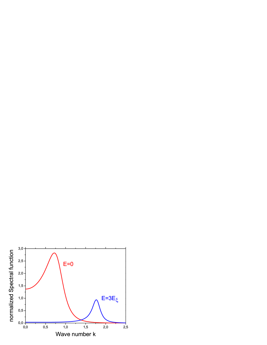
Figure 2: Spectral function, normalized to the total density of states at energy $E$, calculated in the SCBA, for $E=0$ (red) and $E=3$ (blue) and for $U/E_{\xi}^{2}=1$. At small energies it has a large weight at $k=0$ (very cold atoms) and extends up to $k=2$.

3 Bethe-Salpeter equation

We proceed with the calculation of the diffusion constant of the cold atoms, and the possible presence of a mobility edge where it vanishes. With that information we will find how many atoms will be localized. The idealized model we consider is schematically drawn in Figure 3.

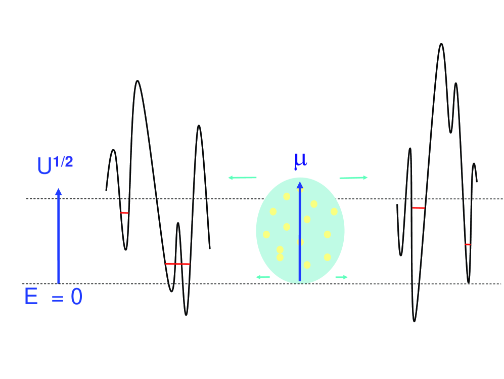
Figure 3: Model of the atomic expansion. The BEC releases noninteracting atoms with kinetic energies between $0$ and its chemical potential $\mu$, that penetrate the disordered speckle potential, with average and its typical fluctuations equal to $\sqrt{U}$. In this work localized states (red) are found only for energies below the average.

The Bethe-Salpeter equation is a rigorous equation for the two-particle Green function mahan . In phase space this object is written as $\Phi_{\mathbf{kk}^{\prime}}(E,t,\mathbf{r})$, which is readily interpreted as the“quantum probability density” for an atom with velocity $\hbar\mathbf{k}/m$ to travel, during the time $t$, from position $\mathbf{r}=0$ to position $\mathbf{r}$ and to achieve the velocity $\hbar\mathbf{k}^{\prime}/m$. Its Fourier-Laplace transform with space-time is written as $\Phi_{\mathbf{kk}^{\prime}}(E,\Omega,\mathbf{q})$. It has two fundamental properties, namely reciprocity, $\Phi_{\mathbf{kk}^{\prime}}(E,\Omega,\mathbf{q})=\Phi_{\mathbf{k^{\prime}k}}(E,\Omega,\mathbf{q})$, and normalization. The last property can be expressed by,

$$\sum_{\mathbf{k}}\Phi_{\mathbf{kk}^{\prime}}(E,\Omega,\mathbf{q}=0)=\frac{-2\mathrm{Im}\,G(E,k^{\prime})}{-i\Omega}$$ (2)

In particular, when also integrating over all energies,

$$\int_{-\infty}^{\infty}\frac{dE}{2\pi}\sum_{\mathbf{k,k^{\prime}}}\Phi_{\mathbf{kk}^{\prime}}(E,\Omega,\mathbf{q}=0) =$$

$$\frac{1}{-i\Omega}\int_{-\infty}^{\infty}{dE}\frac{-1}{\pi}\mathrm{Im}\,G(E,k) = \frac{1}{-i\Omega}$$ (3)

The last equality, needed for later purposes, follows from a general sum rule of the spectral function mahan . This identity guarantees that the total quantum probability for the atom to be somewhere, with some velocity and with some energy, is conserved, and equal to one. The Bethe-Salpeter can be re-written as a quantum-kinetic equation for $\Phi_{\mathbf{kk}^{\prime}}(E,\Omega,\mathbf{q})$. The conservation of quantum probability guarantees the existence of a hydrodynamic diffusion pole. We shall express this as

$$\Phi_{\mathbf{kk}^{\prime}}(E,\Omega,\mathbf{q})=\frac{2}{\sum_{\mathbf{k}}-\mathrm{Im}\,G(E,k)}\,\,\frac{\phi(E,\mathbf{k},\mathbf{q})\phi(E,\mathbf{k}^{\prime},\mathbf{q})}{-i\Omega+D(E)q^{2}}$$ (4)

where

$$\phi(E,\mathbf{k},\mathbf{q})=-\mathrm{Im}\,G(E,k)-i(\mathbf{k}\cdot\mathbf{q})F(E,k)+\mathcal{O}(q^{2}).$$

This expression states that the distribution of atoms in $k$-space at given energy $E$ is essentially governed by the spectral function, with a small correction that supports a current. The front factor in Eq. (4) is imposed by the normalization condition (3). The $k$-integral of $-\mathrm{Im}\,G(E,k)$ is recognized as ($\pi$ times) the density of states (DOS) per unit volume $\rho(E)$. With the correct normalization, we can set $\Omega=0$. The still unknown function $F(p)$ follows from mahan

$$F(E,k) = |G(E,k)|^{2}-\frac{\partial\mathrm{Re}\,G(E,k)}{\partial k^{2}}$$ (5)

$$+ |G(E,k)|^{2}\sum_{\mathbf{k^{\prime}}}\frac{\partial\mathrm{Re}\,G(E,k^{\prime})}{\partial k^{\prime 2}}\frac{\mathbf{k}\cdot\mathbf{k}^{\prime}}{k^{2}}U_{\mathbf{kk}^{\prime}}(E,0)$$

$$+ |G(E,k)|^{2}\sum_{\mathbf{k^{\prime}}}F(E,k^{\prime})\frac{\mathbf{k}\cdot\mathbf{k}^{\prime}}{k^{2}}U_{\mathbf{kk}^{\prime}}(E,0)$$

The irreducible vertex $U_{\mathbf{\mathbf{kk}}^{\prime}}(E,\mathbf{q})$ generalizes the function $U(\mathbf{k}-\mathbf{k}^{\prime})$ defined in the first section to all interference contributions in multiple scattering. Once we have solved for $F(E,k)$, the diffusion constant follows from the Kubo-Greenwood formula mahan ,

$$D(E)=\frac{\hbar}{m}\frac{2}{3}\frac{1}{\pi\rho(E)}\sum_{\mathbf{k}}k^{2}F(E,k)$$ (6)

Note that $D(E)$ is determined by the fourth moment of the distribution $F(E,k)$, which puts a large weight on ”fast” atoms. The order of magnitude of the diffusion constant is governed by the ratio $\hbar/m$ of Planck’s constant and the mass of the atom, the second factor being dimensionless and of order unity at low energies. For ⁸⁷Ru, $\hbar/m\approx 1800$ $\mu$m²/s. The third term in Eq. (5) can be transformed using the exact Ward identity,

$$\Sigma(E,\mathbf{k}+\frac{1}{2}\mathbf{q})-\Sigma^{*}(E,\mathbf{k}-\frac{1}{2}\mathbf{q})={\sum_{\mathbf{k^{\prime}}}}U_{\mathbf{kk}^{\prime}}(E,\mathbf{q})$$

$$\times\left(G(E,\mathbf{k^{\prime}}+\frac{1}{2}\mathbf{q})-G^{*}(E,\mathbf{k^{\prime}}-\frac{1}{2}\mathbf{q})\right)$$ (7)

If this identity is developed linearly in $\mathbf{q}$, and inserted into Eq. (5) , we obtain,

$$F(E,k) = F_{0}(E,k)+\delta_{\mathbf{q}}U(E,k)$$ (8)

$$+ |G(E,k)|^{2}\sum_{\mathbf{k^{\prime}}}F(E,k^{\prime})\frac{\mathbf{k}\cdot\mathbf{k}^{\prime}}{k^{2}}U_{\mathbf{kk}^{\prime}}(E,0)$$

with

$$F_{0}(E,k)\equiv|G(E,k)|^{2}\left(1+\frac{\partial\mathrm{Re}\,\Sigma(E,k)}{\partial k^{2}}\right)-\frac{\partial\mathrm{Re}\,G(E,k)}{\partial k^{2}}$$

$$\delta_{\mathbf{q}}U\equiv|G(E,k)|^{2}\sum_{\mathbf{k}^{\prime}}\mathrm{Im}\,G(E,k^{\prime})\left(2i\frac{\mathbf{k}}{k^{2}}\cdot\frac{\partial}{\partial\mathbf{q}}\right)U_{\mathbf{kk}^{\prime}}(E,\mathbf{q})$$

.

Three levels of analysis exist. First, in the Drude approximation, one neglects all contributions form the BS-equation and one adopts $F(E,p)=F_{0}(E,p)$, including the wave number derivatives. The Drude diffusion constant $D_{d}(E)$ can be used to define a dimensionless Ioffe-Regel type parameter from the relation $D_{d}(E)=\frac{1}{3}(2\hbar/m)k\ell$. Hence,

$$k\ell\equiv\frac{\sum_{\mathbf{k}}k^{2}F_{0}(E,k)}{\sum_{\mathbf{k}}-\mathrm{Im}\,G(E,k)}$$ (9)

For a short-range correlation, the self-energy is independent of $k$ so that $F_{0}(E,k)=2\mathrm{Im}^{2}\,G(E,k)$, and this definition of $k\ell$ coincides with the usual one in terms of $\-\mathrm{Im}\,\Sigma(E)$ pr . For low energies we found in Figure 3 that typically $k\approx 1/\xi$ . If we anticipate that $k\ell\approx 1$ near the mobility edge, we conclude that the mean free path is roughly equal to the correlation length.

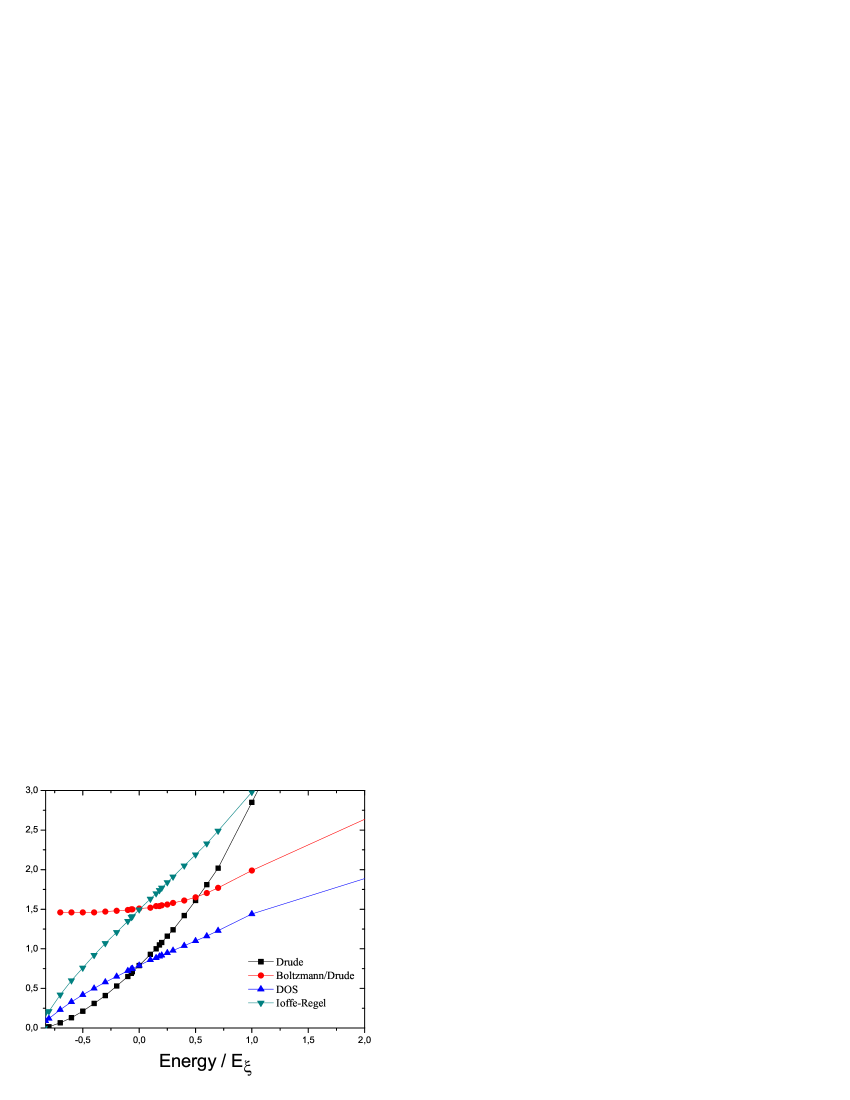
Figure 4: Solution of the BS equations (6) and (8) in the Boltzmann approximation, for a disorder amplitude $U/E_{\xi}^{2}=1$. Shown as a function of energy are the Drude conductivity $\pi\rho(E)D_{d}(E)$, the Ioffe-Regel parameter (9), the DOS that vanishes at the band edge $E/E_{\xi}=-0.83$, and the ratio of Boltzmann and Drude conductivity. Note that $2/3$ times the Ioffe-Regel parameter equals the Drude diffusion constant, expressed in units of $\hbar/m$.

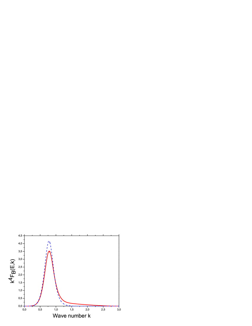
Figure 5: The function $k^{4}F_{B}(E,k)$, solution of the BS-equation for the energy $E/E_{\xi}=-0.06$ in the Boltzmann approximation. The blue dashed line compares it to the Drude approximation $k^{4}F_{0}(E,p)$ defined in Eq. (8), rescaled properly such that both $k$-integrals equal $\sigma_{B}/\sigma_{0}$

The Drude approximation is popular in electron - impurity scattering but clearly inadequate when the scattering is strongly anisotropic, as for the optical speckle. In the Boltzmann approximation we adopt $U_{\mathbf{kk}^{\prime}}=U(\mathbf{k-k}^{\prime})$, i.e. the structure function associated with the optical disorder. Being a function of $\mathbf{k}-\mathbf{k}^{\prime}$ only, it follows that $\delta_{\mathbf{q}}U=0$. Different results are summarized in Figure 4. At low energies Boltzmann and Drude diffusion constant typically differ by a factor $1.5$ as was obtained by Kuhn etal kuhn on the basis of the FBA. For atom energies $E>E_{\xi}$ the Boltzmann diffusion constant rapidly rises since only strong forward scattering can occur. In the region $E=0$, the Ioffe-Regel parameter takes values of the order of $1.5$. We infer from Figure 5 that the solution $F_{B}(E,p)$ is roughly a rescaling of the Drude Ansatz, for which the current is dominated by atoms with velocities $v=0.83\hbar/m\xi$. Nevertheless, a non-negligible fraction of atoms faster than $v=1.5\hbar/m\xi$ contributes to the current (note that $\hbar/m\xi\approx 7$ mm/s for the set-up with Rubidium described above).

We finally consider constructive interferences, and add the most-crossed diagrams to the BS-equation in the spirit of the self-consistent theory of localization. Any observation $D<D_{B}$ must be attributed to constructive interferences. It is well-known that, by reciprocity, these diagrams can be constructed from the solution $\phi(E,\mathbf{k},\mathbf{q})$ of the BS-equation by removing the incoming and outgoing Green’s functions (indicated by a hat), and by time-reversing the bottom line eplbart : $U^{MC}_{\mathbf{kk}^{\prime}}(E,\mathbf{q})=\widehat{\Phi}_{\frac{1}{2}(\mathbf{k}-\mathbf{k}^{\prime}+\mathbf{q})\,\frac{1}{2}(\mathbf{k}^{\prime}-\mathbf{k}+\mathbf{q})}(E,\mathbf{k}+\mathbf{k}^{\prime})$. Using Eq. (4) the two procedures lead to

$$\widehat{\Phi}_{\mathbf{kk}^{\prime}}(E)=\frac{2}{\sigma(E)\mathbf{q}^{2}}\times$$ (10)

$$\left[\mathrm{Im}\Sigma(E,k)\mathrm{Im}\Sigma(E,k^{\prime})\right.+\left.i\mathbf{q}\cdot(I_{kk^{\prime}}(E)\mathbf{k}+I_{k^{\prime}k}(E)\mathbf{k}^{\prime})\right]$$

$$U^{\mathrm{MC}}_{\mathbf{kk}^{\prime}}(E,\mathbf{q})=\frac{2}{\sigma(E)(\mathbf{k}+\mathbf{k}^{\prime})^{2}}\times$$

$$\left[\mathrm{Im}^{2}\Sigma(E,\frac{1}{2}\Delta k)+I_{\Delta k/2,\Delta k/2}(E)i(\mathbf{k}+\mathbf{k}^{\prime})\cdot\mathbf{q}\right]$$

We abbreviated $I_{kk^{\prime}}=F(E,k)\mathrm{Im}\,\Sigma(E,k^{\prime})/|G(E,k)|^{2}$, $\Delta k$ $=|\mathbf{k}-\mathbf{k}^{\prime}|$ and introduced $\sigma(E)=\pi\rho(E)D(E)$, the equivalent of DC-conductivity in electron conduction. We now face the more complicated task of solving Eqs. (8) and (6) simultaneously with $U_{\mathbf{kk}^{\prime}}=U(\mathbf{k}-\mathbf{k}^{\prime})+U^{\mathrm{MC}}_{\mathbf{kk}^{\prime}}$, and of finding out if its extrapolation to small energies leads to a mobility edge where $\sigma(E)=0$. This constitutes a ”self-consistent” problem for the entire function $F(E,k)$, rather than just for its fourth moment, the DC-conductivity.

We first observe that for most-crossed diagrams $\delta_{\mathbf{q}}U\neq 0$. This term does not appear in standard self-consistent theory vw , which relies on moment expansion. Note that it also features ”self-consistently” the function $F(k)/\sigma$, just like the second term in Eq. (8). As can be induced from Eq. (10) the singularity at $\mathbf{k}=-\mathbf{k}^{\prime}$ that generates the (weak) localization is partly compensated by the factor $\mathbf{k}+\mathbf{k}^{\prime}$. We shall therefore ignore it here as well.

The self-consistent equations (8),(6) and (10) can be solved almost analytically when the self-energy is assumed $k$-independent, typically true for zero-range correlations. Without more details we mention that the mobility edge then occurs at $k\ell=1.122$ eplloc . Quite convenient is that, even when scattering extends to infinite wave numbers, our theory does not require an ad-hoc cut-off to eliminate short wave paths that diverge in approximate theories kuhn ; economou . For the speckle correlation, Figure 6 gives the result of the exact numerical solution, obtained by iteration and spline interpolation. This method worked satisfactorily until close to ($\Delta E\approx E_{\xi}/5$) the mobility edge, where the most-crossed diagrams give a diverging contribution. Before that happens, the strong forward scattering of a single scattering competes heavily with the reduction induced by weak localization.

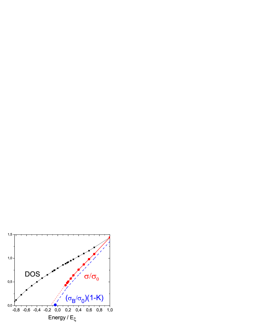
Figure 6: Solution of the BS equation (8) with inclusion of the most-crossed diagrams for a disorder amplitude $U/E_{\xi}^{2}=1$. Shown in red is the ratio of conductivity and Drude conductivity for energies $E>0.15E_{\xi}$ for which our iteration converged. The blue dashed line relies on an approximation discussed in the text and locates the mobility at $E=-0.06E_{\xi}$.

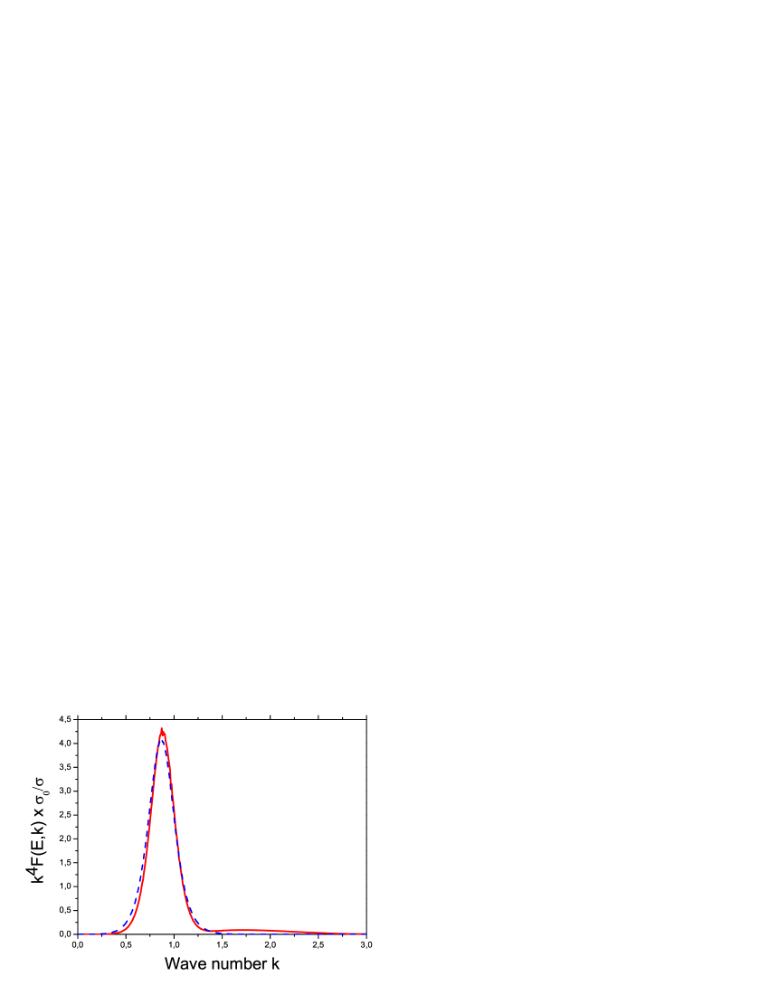
Figure 7: The function $k^{4}F(E,k)$ (in red)), solution of the BS-equation for the energy $E/E_{\xi}=0.15$, compared to the Drude approximation $k^{4}F_{0}(E,p)$ defined in Eq. (8) (blue dashed line). The first has been rescaled by the factor $\sigma_{0}/\sigma$ such that the $k$-integrals of both are equal to one.

To find the location of the mobility edge we shall use the following approximation. In Figure 7 we see that at $E/E_{\xi}=0.15$ the solution $F(E,k)/\sigma$ is closely approximated by $F_{0}(E,k)/\sigma_{0}$ (both have their fourth moment normalized to one). This equivalence is physically reasonable since it implies that all atoms with energy $E$ undergo the same reduction in diffusion, but keep the same velocity distribution as found in the Drude picture. If we insert $F_{0}(E,k)$ in the left hand side of Eq. (8) and integrate over $k$ we can derive the simple relation $\sigma/\sigma_{B}\approx 1-K(E)$ that is reminiscent of standard self-consistent theory vw . The parameter $K$ is found to be,

$$K(E)=-\frac{4}{3\sigma_{d}^{2}(E)}\sum_{\mathbf{kk}^{\prime}}F_{0}(E,k^{\prime})\frac{\mathbf{k}\cdot\mathbf{k}^{\prime}}{(\mathbf{k}+\mathbf{k}^{\prime})^{2}}\times$$

$$\mathrm{Im}^{2}\Sigma\left(E,\frac{1}{2}|\mathbf{k}-\mathbf{k}^{\prime}|\right)|G(E,k)|^{2}$$ (11)

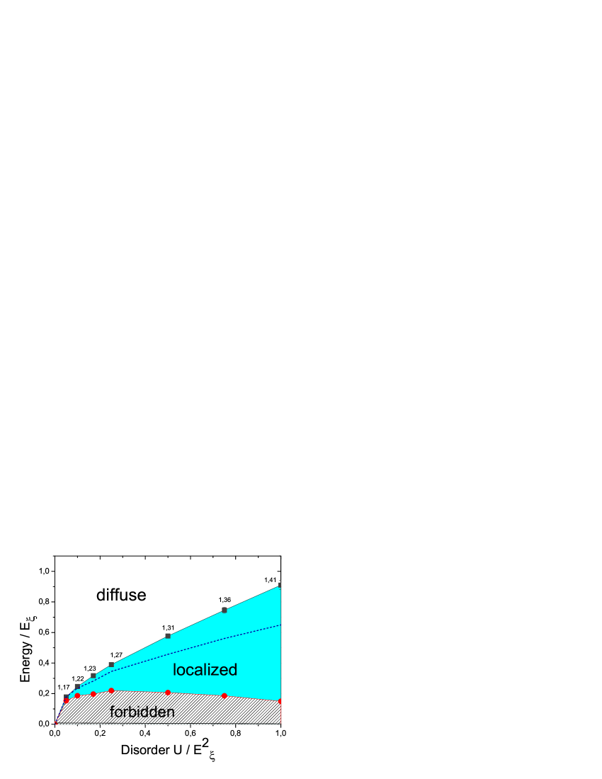
Figure 8: Band edge and mobility edge as a function of the disorder strength $U$, all expressed in the energy $E_{\xi}$. Contrary to the former figures the energy scale has been shifted by the average potential $\sqrt{U}$ of the potential energy so that a direct comparison can be made to the chemical potential $\mu>0$, and the criterion $E_{c}-E_{b}\approx 0.5U/E_{\xi}$ found by Ref.kuhn (blue dashed). The numbers around the mobility edge reveal the small variation of the Ioffe-Regel parameter (9). The exclusion of small energies is likely to be an artifact of the SCBA and we expect strongly localized Lifshits-type states with small DOS.

For $U/E^{2}_{\xi}=1$, this approximation locates the mobility edge ($K=1$) at $E/E_{\xi}=-0.06$ ($0.94$ when we shift energies over $\sqrt{U}$ as in Fig 8). Upon inspecting the numerically exact solution in Figure 8, we suspect that the real mobility edge is located somewhat lower, near $E/E_{\xi}=-0.1$. For smaller disorder we found that the approximation becomes better. It is in principle possible to obtain numerically the function $F(E,p)/\sigma$ as $\sigma\rightarrow 0$ and calculate more precisely the location of mobility edge, but this is beyond the scope of this paper. In Figure 8 we show the different energies for different strengths of the disorder. If we apply the criterion found in Ref kuhn , $k\ell_{B}=0.95$ (dashed line in Figure 8), localization would occur at smaller energies, around $E/E_{\xi}=-0.35$ ($0.65$ in Fig. 8) for $U/E^{2}_{\xi}=1$. This approach expresses the general trend well but is clearly somewhat pessimistic, probably because their choice of the ad-hoc wave number cut-off to calculate the most-crossed diagrams underestimates $K$. Note that all localized states occur below the average of the potential landscape. Unlike in 1D, we find no regime with atoms fast enough to traverse the potential barriers, but to become localized purely by constructive interferences, without the assistance of tunneling.

A final important question is how many atoms will be localized, given an initial velocity distribution that is determined by the expansion of the BEC after eliminating the trap. We emphasize that according to the scenario sketched in Fig. 3, the chemical potential $\mu$ of the BEC does not represent the energy of the atom inside the disordered potential, but rather the distribution of incident kinetic energies. If this distribution is denoted by $\phi_{\mu}(\mathbf{k})$, it follows from Eq. (4) that the fraction of localized atoms, regardless of their final velocity or position, is given by

$$\int_{E_{b}}^{E_{c}}\frac{dE}{2\pi}\sum_{\mathbf{k,k^{\prime}}}\Phi_{\mathbf{kk}^{\prime}}(E,t,\mathbf{q}=0)\phi_{\mu}(\mathbf{k}^{\prime})$$

$$=\int_{E_{b}}^{E_{c}}{dE}\sum_{\mathbf{k^{\prime}}}\frac{-1}{\pi}\mathrm{Im}\,G(E,k^{\prime})\phi_{\mu}(\mathbf{k}^{\prime})$$ (12)

Castin and Dum yvan showed that after the free expansion $\phi_{\mu}(k)\sim 1-k^{2}/k^{2}_{\mu}$ and zero for $k>k_{\mu}$, where the maximum wave number $k_{\mu}=\sqrt{\mu/E_{\xi}}$. The fraction of localized atoms is thus determined by the number of microscopic states below the mobility edge whose kinetic energies are smaller than $\mu$. In this discussion it is convenient to make the zero of the energy scale the same for $\mu$ and $E$, as was already done already in Figure 8, shifting the localized region to positive energies. In present (1D) experiments is $U/E_{\xi}^{2}=1$ and $\mu\approx E_{\xi}$ which is only slightly above the 3D mobility edge. One might perhaps expect most atoms to be localized. Our calculations clearly show that the distribution of atom energies is quite different from $\phi_{\mu}(\mathbf{k})$. This (normalized) distribution $F(E)$ is given by the wave number integral in Eq. (10) and is shown in Figure 9. For $\mu\ll E_{\xi}$ it reduces to the spectral function at $k=0$, independent of $\phi_{\mu}(k)$. Even for small $\mu$, many atoms achieve energies $E>E_{c}$ ($40\,\%$ for $U/E^{2}_{\xi}=1$) and are delocalized. This number agrees well with predictions based on zero-range correlations in which case $45\,\%$ was found to be localized for $\mu\ll E_{c}$ anna . The fraction of delocalized atoms further decreases as the chemical potential rises (Figure 10), with only $35\,\%$ localized for $\mu=E_{\xi}$. Even if we choose $\mu>\sqrt{U}$, the atoms that localize have energies $E<\sqrt{U}$.

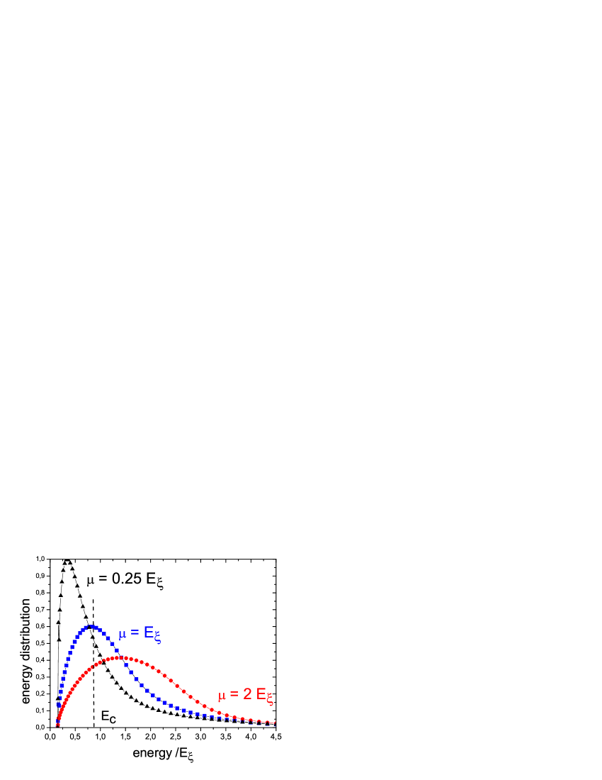
Figure 9: Energy distributions of the atoms inside the disordered speckle potential, for different chemical potentials of the BEC from which they were released and $U/E_{\xi}^{2}=1$. They all exhibit a tail of relatively fast atoms ($E>E_{\xi}$) that extends beyond the mobility edge $E_{c}$.

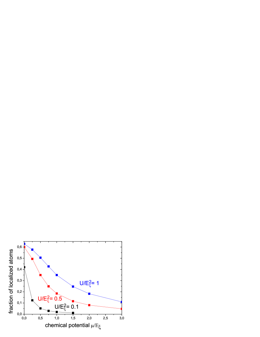
Figure 10: Fraction of localized atoms as a function of chemical potential, for different amplitudes of the disorder.

In conclusion, we have calculated the phase diagram for localization of cold atoms in a 3D speckle potential, using the self-consistent Born approximation and the self-consistent theory of localization. The mobility edge is characterized by a Ioffe-Regel type parameter that varies between $1.2$ and $1.4$. Depending on the chemical potential of the BEC, typically $35\,\%$ to $60\,\%$ of the atoms are localized. The self-consistent Born approximation deals already much better with the long-range correlations and the broadness of the spectral function than the first Born approximation, but does not discriminate between different statistics of the disorder. Yet, the mobility edge of the tight-binding model is known to depend on that kroha . It would be very interesting to apply a recently proposed method schindler to calculate the self-energy of the atoms more precisely. The theory presented in this work can then be used straightforwardly to find the mobility edge.

- (1) A. Lagendijk, B.A. van Tiggelen and D.S. Wiersma, Physics Today 62, 24 (2009).
- (2) A. Aspect and M. Inguscio, Physics Today 62, 30 (2009).
- (3) P.W. Anderson, Phys. Rev. 109, 1492 (1958).
- (4) B. Kramer and A. MacKinnon, Rep. Prog. Phys. 56, 1469 (1993).
- (5) D.S. Wiersma, P. Bartolini, A. Lagendijk and R. Righini, Nature 390, 671 (1997).
- (6) H. Hu, A. Strybulevych, J.H. Page, S.E. Skipetrov, and B.A. van Tiggelen, Nature Physics 4, 945 (2008).
- (7) J. Chabé, G. Lemarie, B. Gremaud, D. Delande, P. Szriftgiser, and J. Garreau, Phys. Rev. Let. 101, 255702 (2008).
- (8) E. Abrahams, P.W. Anderson, D.C. Licciardello and T.V. Ramakrishnan, Phys. Rev. Lett. 42, 673 (1979).
- (9) J.T Edwards and D. Thouless, J. Phys. C 5, 807 (1972).
- (10) D. Vollhardt and P. Wölfle, Selfconsistent theory of Anderson Localization, in: Electronic Phase Transitions, eds. W. Hanke and Ya. V. Kopaev (North-Holland, Amsterdam, 1992).
- (11) H. Kroha,T. Kopp, and P. W ölfle, Phys. Rev. B 41,888 (1990).
- (12) G. Roati etal., Nature 453, 895 (2008); J. Billy etal, ibid 891 (2008).
- (13) L. Sanchez-Palencia etal, Phys. Rev. Lett. 98, 210401 (2007); P. Lugan, A. Aspect, L. Sanchez-Palencia, D. Delande, B. Grémaud, C. Müller and C. Miniatura, Phys. Rev. A 80, 023605 (2009).
- (14) R.C. Kuhn, C. Miniatura, D. Delande, O. Sigwarth, and C.M. Müller, Phys. Rev. Lett. 98, 21041 (2007); New J. Phys. 9, 161 (2007).
- (15) A. Lagendijk and B.A. van Tiggelen, Phys. Rep. 270, 143 (1996).
- (16) N.E. Cusack, The Physics of Structurally Disordered Matter (IOPP, 1987).
- (17) S.E. Skipetrov, A. Minguzzi, B.A. van Tiggelen and B. Shapiro, Phys. Rev. Lett. 100, 165301 (2008).
- (18) G.D. Mahan, Many-Particle Physics (Plenum, New York, 1981), section 7.1.C.
- (19) B.A. van Tiggelen, D.S. Wiersma and A. Lagendijk, Europhys. Lett. 30, 1 (1995).
- (20) B.A. van Tiggelen, A. Lagendijk, A. Tip and G.F. Reiter, Europhys. Lett. 15, 535 (1991). In this work the slightly different value was obtained from a less rigorous moment expansion.
- (21) E.N. Economou, C.M. Soukoulis, and A.D. Zdetsis, Phys. Rev. B 30, 1686 (1984).
- (22) Y. Castin and R. Dum, Phys. Rev. Lett. 77, 5315 (1996).
- (23) R. Zimmermann and Ch. Schindler, Phys. Rev. B 80, 144202 (2009).