Distance $k$-sectors exist

Abstract

The bisector of two nonempty sets $P$ and $Q$ in $\mathbb{R}^{d}$ is the set of all points with equal distance to $P$ and to $Q$. A distance $k$-sector of $P$ and $Q$, where $k\geq 2$ is an integer, is a $(k-1)$-tuple $(C_{1},C_{2},\ldots,C_{k-1})$ such that $C_{i}$ is the bisector of $C_{i-1}$ and $C_{i+1}$ for every $i=1,2,\ldots,k-1$, where $C_{0}=P$ and $C_{k}=Q$. This notion, for the case where $P$ and $Q$ are points in $\mathbb{R}^{2}$, was introduced by Asano, Matoušek, and Tokuyama, motivated by a question of Murata in VLSI design. They established the existence and uniqueness of the distance trisector in this special case. We prove the existence of a distance $k$-sector for all $k$ and for every two disjoint, nonempty, closed sets $P$ and $Q$ in Euclidean spaces of any (finite) dimension (uniqueness remains open), or more generally, in proper geodesic spaces. The core of the proof is a new notion of $k$-gradation for $P$ and $Q$, whose existence (even in an arbitrary metric space) is proved using the Knaster–Tarski fixed point theorem, by a method introduced by Reem and Reich for a slightly different purpose.

1 Introduction

The bisector of two nonempty sets $X$ and $Y$ in Euclidean space, or in an arbitrary metric space $(M,\mathrm{dist})$, is defined as

$$\operatorname{bisect}(X,Y)=\{\,z\in M:\mathrm{dist}(z,X)=\mathrm{dist}(z,Y)\,\},$$ (1)

where $\mathrm{dist}(z,X)=\inf_{x\in X}\mathrm{dist}(z,x)$ denotes the distance of $z$ from a set $X$.

Let $k\geq 2$ be an integer and let $P$, $Q$ be disjoint nonempty sets in $M$ called the sites. A distance $k$-sector (or simply $k$-sector) of $P$ and $Q$ is a $(k-1)$-tuple $(C_{1},\dots,C_{k-1})$ of nonempty subsets of $M$ such that

$$C_{i} =\operatorname{bisect}(C_{i-1},C_{i+1}), i=1,\ldots,k-1,$$ (2)

where $C_{0}=P$ and $C_{k}=Q$ (see Figures 1 and 2).

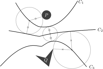
Figure 1: A $4$-sector $(C_{1},C_{2},C_{3})$ of sets $P$ and $Q$ in Euclidean plane. Each point on the curve $C_{i}$ is at the same distance from $C_{i-1}$ and $C_{i+1}$. Note that $C_{2}$ is not the bisector of $P$ and $Q$.

Distance $k$-sectors were introduced by Asano et al. [3], motivated by a question of Murata from VLSI design: Suppose that we are given a topology of a circuit layer, and we need to put $k-1$ wires through a corridor between given two sets of obstacles (modules and other wires) on the board. The circuit will have a high failure probability if the gaps between the wires are narrow. Which curves should the wires follow in order to minimize the failure probability? If $k=2$, the curve should be the distance bisector; in general, each curve should be the bisector of its adjacent pair of curves, as stated in the definition of a $k$-sector.

$P$                           $Q$                           

Figure 2: A $7$-sector of two singleton sets $P$ and $Q$ in Euclidean plane.

A similar problem occurs also in designing routes of $k-1$ autonomous robots moving in a narrow polygonal corridor. Each robot has its own predetermined route (say, it is drawn on the floor with a coloured tape that the robot can recognize) and tries to follow it. We want to design the routes to be far away from each other so that the robots can easily avoid collision.

Despite its innocent definition, it is nontrivial to find a $k$-sector even in Euclidean plane. The bisector of two point sites $P$ and $Q$ in $\mathbb{R}^{2}$ is a line, and an elementary geometric argument shows that there is a distance $4$-sector of them consisting of a straight line and two parabolas. However, the problem was not investigated for other values of $k$ until Asano et al. [3] proved the existence and uniqueness of the $3$-sector of two points in Euclidean plane. Chun et al. [4] extended this to the case where $Q$ is a line segment.

We give the first proof of existence of distance $k$-sectors in Euclidean spaces for a general $k$. This improves on the previous proofs in generality and simplicity even for $k=3$.

Main Theorem.

Every two disjoint nonempty closed sets $P$ and $Q$ in Euclidean space $\mathbb{R}^{d}$, or more generally, in a proper geodesic metric space, have at least one $k$-sector.

Here, a metric space $(M,\mathrm{dist})$ is called proper if all closed balls are compact. It is called geodesic if for every two distinct points $x$, $y\in M$ there is a metric segment in $M$ connecting them, i.e., an isometric mapping $\gamma\colon[a,b]\to M$ of an interval $[a,b]\subset\mathbb{R}$ with $\gamma(a)=x$ and $\gamma(b)=y$. In particular, a convex subset of a normed space is a geodesic metric space. Another example is the surface of a sphere, where the distance between two points is measured by the length of the shortest path on the surface connecting them. Geodesic metric spaces are a reasonably general class of metric spaces in which our arguments go through, although one could probably make up even more general conditions.

Let us remark that if $\mathrm{dist}(P,Q)>0$ and $k=3$, then the properness assumption can be omitted; see [8] for a proof.

On the other hand, $k$-sectors need not exist in arbitrary metric spaces. A simple example for $k=3$ is the subspace $M=\{-1,0,1\}$ of the real line, $P=\{1\}$, and $Q=\{-1\}$.

From now on, unless otherwise noted, subscripts $i$ and $j$ range over $1$, …, $k-1$; for example, $(C_{i})_{i}$ stands for the $k$-tuple $(C_{1},\dots,C_{k-1})$.

Gradations

One of the main steps in the proof of the main theorem is introducing the notion of a $k$-gradation of $P$ and $Q$, which is related to a $k$-sector but easier to work with. First, for nonempty sets $X$, $Y$ in a metric space $(M,\mathrm{dist})$, we define the dominance region of $X$ over $Y$ by

$$\operatorname{dom}(X,Y)=\{\,z\in M:\mathrm{dist}(z,X)\leq\mathrm{dist}(z,Y)\,\}.$$ (3)

A $k$-gradation between nonempty subsets $P$ and $Q$ of $M$ is a $(k-1)$-tuple $(R_{i},S_{i})_{i}$ of pairs of subsets of $M$ satisfying

$$R_{i} =\operatorname{dom}(R_{i-1},S_{i+1}), S_{i} =\operatorname{dom}(S_{i+1},R_{i-1}), i=1,\ldots,k-1,$$ (4)

where $R_{0}=P$ and $S_{k}=Q$.

Using the Knaster–Tarski fixed point theorem [9], we prove in Section 2 that $k$-gradations always exist:

Proposition 1.

For every nonempty sets $P$ and $Q$ in an arbitrary metric space $(M,\mathrm{dist})$, there exists at least one $k$-gradation.

The idea of applying the Knaster–Tarski theorem to a similar setting is from [7], where it is used to prove the existence of double zone diagrams. A slight modification of Proposition 1 also holds in the more general setting of m-spaces [7].

In Section 3, we establish the following connection between $k$-gradations and $k$-sectors.

Proposition 2.

Let $P$, $Q$ be nonempty, disjoint, closed sets in a proper geodesic metric space. Then a $(k-1)$-tuple $(C_{i})_{i}$ of sets is a $k$-sector of $P$ and $Q$ if and only if

$$C_{i} =R_{i}\cap S_{i}, i=1,\dots,k-1$$ (5)

for some $k$-gradation $(R_{i},S_{i})_{i}$ between $P$ and $Q$.

For instance, the $k$-sectors $(C_{i})_{i}$ in Figures 1, 2 and 3 correspond to the $k$-gradations $(R_{i},S_{i})_{i}$ where each $R_{i}$ is the union of $C_{i}$ and the region above it, and each $S_{i}$ is the union of $C_{i}$ and the region below it.

The main theorem is an immediate consequence of Propositions 1 and 2.

$3$-gradations and zone diagrams

A zone diagram of $P$, $Q$ is, according to the general definition of Asano et al. [2], a pair of sets $(A,B)$ such that $A=\operatorname{dom}(P,B)$ and $B=\operatorname{dom}(Q,A)$. By comparing the definitions, we can see that if $((R_{1},S_{1}),(R_{2},S_{2}))$ is a $3$-gradation for $P$, $Q$, then $(R_{1},S_{2})$ is a zone diagram of $P$, $Q$. Conversely, given a zone diagram $(A,B)$, we can set $R_{1}:=A$, $S_{2}:=B$, $R_{2}:=\operatorname{dom}(R_{1},Q)$, $S_{1}:=\operatorname{dom}(S_{2},P)$ to obtain a $3$-gradation (we note that $R_{2}$ and $S_{1}$ are uniquely determined by $R_{1}$ and $S_{2}$).

The existence of zone diagrams of arbitrary two nonempty sets in an arbitrary metric space (and even in the still more general setting of m-spaces) was proved by Reem and Reich [7, Theorem 5.6]. By the above, it immediately implies the existence of $3$-gradations, a special case of Proposition 1.

Uniqueness

Kawamura et al. [6] (also see [5] for a preliminary version) proved the existence and uniqueness of zone diagrams in $\mathbb{R}^{d}$ (for finitely many closed and pairwise separated sites) under the Euclidean distance, and more generally, under any smooth and uniformly convex norm. By Proposition 2, this implies the uniqueness of trisectors under the same conditions. This is the most general uniqueness result for $k$-sectors we are aware of.

For general metrics, $k$-sectors need not be unique. A simple example, for the $\ell_{1}$ metric in the plane (given by $\mathrm{dist}(x,y)=|x_{1}-y_{1}|+|x_{2}-y_{2}|$), is shown in Figure 3; essentially, it was discovered by Asano and Kirkpatrick [1]. The set $C_{1}$ is a polygonal curve, while $C_{2}$ is “fat”, consisting of two straight segments and two quadrants. A different trisector is obtained as a mirror reflection of the one shown.

Figure 3: A $3$-sector $(C_{1},C_{2})$ of $P$ and $Q$ under the $\ell_{1}$ norm.

Thus, uniqueness of $k$-sectors requires some geometric assumptions on the underlying metric space. We will further comment on this issue in Section 4.

Construction of $k$-sectors

Our existence proof for $k$-sectors, based on the Knaster–Tarski theorem, is somewhat nonconstructive. In Section 4, we discuss a more constructive approach, which re-establishes Proposition 1 under stronger assumptions, but which yields an iterative algorithm (in a similar spirit as in [2]). We have no rigorous results about the speed of its convergence, but in practice it has been used successfully for approximating $k$-sectors and drawing pictures such as Figure 1. Such computations also support our belief that $k$-sectors in Euclidean spaces are unique, at least for two point sites in the plane.

2 The existence of $k$-gradations

Here we prove Proposition 1. A set $\mathcal{L}$ equipped with a partial order $\mathord{\leq}$ is called a complete lattice if every subset $\mathcal{D}\subseteq\mathcal{L}$ has an infimum $\bigwedge\mathcal{D}$ (the greatest $x\in\mathcal{L}$ such that $x\leq y$ for all $y\in\mathcal{D}$) and a supremum $\bigvee\mathcal{D}$ (the least $x\in\mathcal{L}$ such that $x\geq y$ for all $y\in\mathcal{D}$). We say that a function $F\colon\mathcal{L}\to\mathcal{L}$ on a complete lattice $\mathcal{L}$ is monotone if $x\leq y$ implies $F(x)\leq F(y)$.

Knaster–Tarski Theorem ([9]).

Every monotone function on a complete lattice has a fixed point.

The proof of this theorem is simple: It is routine to verify that the least and the greatest fixed points of a monotone function $F\colon\mathcal{L}\to\mathcal{L}$ are given by

$$\bigwedge\{\,x\in\mathcal{L}:x\geq F(x)\,\}, \bigvee\{\,x\in\mathcal{L}:x\leq F(x)\,\},$$ (6)

respectively.

Proof of Proposition 1..

Let $\mathcal{L}$ be the set of all $(k-1)$-tuples $(R_{i},S_{i})_{i}$ of pairs of subsets of the considered metric space $M$ satisfying $R_{i}\supseteq P$, $S_{i}\supseteq Q$ and $R_{i}\cup S_{i}=M$. We define the order $\mathord{\leq}$ on $\mathcal{L}$ by setting $(R_{i},S_{i})_{i}\leq(R^{\prime}_{i},S^{\prime}_{i})_{i}$ if $R_{i}\subseteq R^{\prime}_{i}$ and $S_{i}\supseteq S^{\prime}_{i}$ for all $i=1,\ldots,k-1$. It is easy to see that $\mathcal{L}$ with this order $\mathord{\leq}$ is a complete lattice in which the infimum and supremum of $\mathcal{D}\subseteq\mathcal{L}$ are given by

$$\bigwedge\mathcal{D} =\Bigl{(}\bigcap_{(R_{j},S_{j})_{j}\in\mathcal{D}}R_{i},\bigcup_{(R_{j},S_{j})_{j}\in\mathcal{D}}S_{i}\Bigr{)}_{i}, \bigvee\mathcal{D} =\Bigl{(}\bigcup_{(R_{j},S_{j})_{j}\in\mathcal{D}}R_{i},\bigcap_{(R_{j},S_{j})_{j}\in\mathcal{D}}S_{i}\Bigr{)}_{i}.$$ (7)

We define $F\colon\mathcal{L}\to\mathcal{L}$ by

$$F\bigl{(}(R_{i},S_{i})_{i}\bigr{)}=\bigl{(}\operatorname{dom}(R_{i-1},S_{i+1}),\operatorname{dom}(S_{i+1},R_{i-1})\bigr{)}_{i},$$ (8)

where $R_{0}=P$ and $S_{k}=Q$. It is easy to see that $F$ is well-defined and monotone. By the Knaster–Tarski Theorem, $F$ has a fixed point, which is a $k$-gradation by definition. ∎

3 Dominance regions, $k$-gradations, and $k$-sectors

The goal of this section is to prove Proposition 2. We write $\partial Z$ for the boundary of a closed set $Z$. We begin with observing that, for arbitrary nonempty sets $X$, $Y$ in any metric space, the set $\operatorname{bisect}(X,Y)=\operatorname{dom}(X,Y)\cap\operatorname{dom}(Y,X)$ contains $\partial\operatorname{dom}(X,Y)$. Moreover, if the metric space is geodesic (and hence connected), then $\operatorname{bisect}(X,Y)$ is nonempty. For otherwise, $\operatorname{dom}(X,Y)$ and $\operatorname{dom}(Y,X)$ would be two disjoint closed sets covering the whole space.

Lemma 3.

Let $X$, $Y$, $Z$ be nonempty closed sets in a proper geodesic metric space. Note that $D=\operatorname{dom}(X,Y)$ and $C=\operatorname{bisect}(X,Y)$ are nonempty. If $D$ and $Z$ are disjoint, then

1. $\operatorname{dom}(D,Z)=\operatorname{dom}(C,Z)$, $\operatorname{dom}(Z,D)=\operatorname{dom}(Z,C)$,

2. $\operatorname{bisect}(D,Z)=\operatorname{bisect}(C,Z)$.

Proof.

Part (b) follows from (a) using $\operatorname{bisect}(X,Y)=\operatorname{dom}(X,Y)\cap\operatorname{dom}(Y,X)$.

To show (a), we claim that

$$\mathrm{dist}(a,Z) >\mathrm{dist}(a,C) \text{for all}\ a\in D.$$ (9)

Indeed, let $z\in Z$ be a point attaining the distance to $a$; i.e., $\mathrm{dist}(a,z)=\mathrm{dist}(a,Z)$ (the distance is attained since the intersection of $Z$ with the ball of radius $2\mathrm{dist}(a,Z)$ around $a$ is compact). There is a segment connecting $a$ and $z$—that is, a metric segment (see the definition following the Main Theorem); for $\mathbb{R}^{d}$ this simply means a line segment. The segment is a connected set containing both $a\in D$ and $z\notin D$, so it meets $\partial D$, and thus also $C$, at some point, say $c$. Hence, $\mathrm{dist}(a,z)=\mathrm{dist}(a,c)+\mathrm{dist}(c,z)>\mathrm{dist}(a,c)\geq\mathrm{dist}(a,C)$. We also have

$$\mathrm{dist}(a,C) =\mathrm{dist}(a,D) \text{for all}\ a\notin D.$$ (10)

For let $d\in D$ be arbitrary. Again, there is a segment connecting $a$ and $d$, and it meets $\partial D$, and thus also $C$, at some point, say $c$. Hence, $\mathrm{dist}(a,d)=\mathrm{dist}(a,c)+\mathrm{dist}(c,d)\geq\mathrm{dist}(a,c)\geq\mathrm{dist}(a,C)$. Since $C\subseteq D$, this proves (10).

The first part of (a) comes as follows: Points $a\in D$ belong both to $\operatorname{dom}(D,Z)$ and, by (9), to $\operatorname{dom}(C,Z)$; other points $a\notin D$ belong to $\operatorname{dom}(D,Z)$ and $\operatorname{dom}(C,Z)$ at the same time by (10).

The second part is similar: Points $a\in D$ belong neither to $\operatorname{dom}(Z,D)$ nor to $\operatorname{dom}(Z,C)$ by (9); other points $a\notin D$ belong to $\operatorname{dom}(Z,D)$ and $\operatorname{dom}(Z,C)$ at the same time by (10). ∎

Now we proceed with $k$-gradations. Let $(R_{i},S_{i})_{i}$ be a $k$-gradation for $P$ and $Q$ as in Proposition 2. We observe that $R_{i}\cup S_{i}$ is the whole space and that

$$P=R_{0}\subseteq R_{1}\subseteq\dots\subseteq R_{k-1}, S_{1}\supseteq S_{2}\supseteq\dots\supseteq S_{k}=Q,$$ (11)

because $X\subseteq\operatorname{dom}(X,Y)$.

Lemma 4.

Let $P$, $Q$ be nonempty, disjoint, closed sets in an arbitrary metric space.

1. If $(C_{i})_{i}$ is a $k$-sector of $C_{0}=P$ and $C_{k}=Q$, then $C_{i-1}$ and $C_{i+1}$ are disjoint for each $i=1$, …, $k-1$.

2. If $(R_{i},S_{i})_{i}$ is a $k$-gradation between $R_{0}=P$ and $S_{k}=Q$, then $R_{i}$ and $S_{j}$ are disjoint for each $i$ and $j$ with $0\leq i<j\leq k$.

Proof.

Suppose that there is a point $a\in C_{i-1}\cap C_{i+1}$. Since $\mathrm{dist}(a,C_{i-1})=0=\mathrm{dist}(a,C_{i+1})$, we have $a\in\operatorname{bisect}(C_{i-1},C_{i+1})=C_{i}$. Since $P$ and $Q$ are disjoint, either $a\notin P$ or $a\notin Q$. By symmetry, we may assume $a\notin P$. Let $i^{-}$ be the smallest such that $a\in C_{j}$ for all $j=i^{-}$, …, $i$. Then $a\in C_{i^{-}+1}\setminus C_{i^{-}-1}$, contradicting $a\in C_{i^{-}}=\operatorname{bisect}(C_{i^{-}-1},C_{i^{-}+1})$.

For (ii), suppose that there is a point $a\in R_{i}\cap S_{j}$ for some $i<j$. Since $P$ and $Q$ are disjoint, either $a\notin P$ or $a\notin Q$. By symmetry, we may assume $a\notin P$. Retake $i$ to be the smallest such that $a\in R_{i}$. Then $a\notin R_{i-1}$ and $a\in S_{j}\subseteq S_{i+1}$, contradicting $a\in R_{i}=\operatorname{dom}(R_{i-1},S_{i+1})$. ∎

Proof of Proposition 2..

For one direction, let $(R_{i},S_{i})_{i}$ be a $k$-gradation and let $C_{i}=R_{i}\cap S_{i}$ for each $i=1$, …, $k-1$. Then $C_{i}=\operatorname{dom}(R_{i-1},S_{i+1})\cap\operatorname{dom}(S_{i+1},R_{i-1})=\operatorname{bisect}(R_{i-1},S_{i+1})$ is nonempty. Moreover, this equals $\operatorname{bisect}(C_{i-1},C_{i+1})$ by Lemma 3(b), because $R_{i-1}$ and $S_{i+1}$ are disjoint according to Lemma 4(ii).

For the other direction, we suppose that $(C_{i})_{i}$ is a $k$-sector. Let $R_{i}=\operatorname{dom}(C_{i-1},C_{i+1})$ and $S_{i}=\operatorname{dom}(C_{i+1},C_{i-1})$ for each $i=1$, …, $k-1$. Then $C_{i}=R_{i}\cap S_{i}$ by the definition of a $k$-sector. By Lemma 4(i), we have $R_{i}\cap C_{i+1}=\emptyset$, and similarly $S_{i+1}\cap C_{i}=\emptyset$. Therefore, $R_{i}\cap S_{i+1}$ is disjoint from $C_{i}\cup C_{i+1}\supseteq\partial R_{i}\cup\partial S_{i+1}\supseteq\partial(R_{i}\cap S_{i+1})$. This means that $R_{i}\cap S_{i+1}$ has an empty boundary, and thus is itself empty, because the whole space is geodesic and hence connected. By this and the fact that $R_{i}\cup S_{i}$ covers the whole space, we have $P\subseteq R_{1}\subseteq\cdots\subseteq R_{k-1}$ and $S_{1}\supseteq S_{2}\supseteq\cdots\supseteq S_{k-1}\supseteq Q$. Because $R_{i}$ and $S_{i+1}$ are disjoint, so are $R_{i-1}$ and $S_{i+1}$. This allows us to apply Lemma 3(a), which yields $\operatorname{dom}(R_{i-1},S_{i+1})=\operatorname{dom}(C_{i-1},C_{i+1})=R_{i}$ and similarly $\operatorname{dom}(S_{i+1},R_{i-1})=S_{i}$. ∎

The following example shows that the assumption of the space being geodesic cannot be dropped. Consider the distance on $\mathbb{R}$ defined by $\mathrm{dist}(x,y)=f(\lvert x-y\rvert)$, where $f$ is given by

$$f(r)=\begin{cases}r&\text{if}\ r\leq 1,\\ 1&\text{if}\ 1\leq r\leq 2,\\ r/2&\text{if}\ r\geq 2.\end{cases}$$ (12)

Thus, $d$ is almost like the usual metric, except that it “thinks of any distance between $1$ and $2$ as the same.” Then there is no trisector between $P=(-\infty,0]$ and $Q=[1,+\infty)$ (whereas there is a gradation by Proposition 1). For suppose that $(C_{1},C_{2})$ is a trisector. By Lemma 4(i), the set $C_{2}$ cannot overlap $P$ or $Q$, so it is a nonempty subset of $(0,1)$. Hence, the point $2$ is equidistant from $C_{2}$ and $P$, and thus belongs to $C_{1}$. This contradicts Lemma 4(i).

4 Drawing $k$-sectors

Here we provide a more constructive proof of the existence of $k$-gradations, but only under stronger assumptions than in Proposition 1. Later we discuss how this approach can be used for approximate computation of bisectors. We write $\overline{X}$ for the closure of a set $X$.

Proposition 5.

Suppose that $P$ and $Q$ are disjoint nonempty closed sets in $\mathbb{R}^{d}$ with the Euclidean norm (or, more generally, with an arbitrary strictly convex norm). Let the lattice $\mathcal{L}$ and the function $F\colon\mathcal{L}\to\mathcal{L}$ be as in the the proof of Proposition 1 (Section 2). Let $(R^{0}_{i},S^{0}_{i})_{i}$ be an arbitrary element of $\mathcal{L}$ with $(R^{0}_{i},S^{0}_{i})_{i}\leq F((R^{0}_{i},S^{0}_{i})_{i})$. Define $(R^{n+1}_{i},S^{n+1}_{i})_{i}:=F((R^{n}_{i},S^{n}_{i})_{i})$ for each $n\in\mathbb{N}$ (thus, $(R^{0}_{i},S^{0}_{i})_{i}\leq(R^{1}_{i},S^{1}_{i})_{i}\leq(R^{2}_{i},S^{2}_{i})_{i}\leq\cdots$), and let $(R^{\infty}_{i},S^{\infty}_{i})_{i}=\bigvee\{\,(R^{n}_{i},S^{n}_{i})_{i}:n\in\mathbb{N}\,\}$. Then $(\overline{R^{\infty}_{i}},S^{\infty}_{i})_{i}$ is a $k$-gradation.

We begin proving this proposition. We write $R^{n}_{0}=P$ and $S^{n}_{k}=Q$ for each $n\in\mathbb{N}\cup\{\infty\}$.

Lemma 6.

For any disjoint nonempty closed sets $X$, $Y$ in $\mathbb{R}^{d}$ with the Euclidean metric (or with a strictly convex norm), $\operatorname{dom}(Y,X)=\overline{\mathbb{R}^{d}\setminus\operatorname{dom}(X,Y)}$.

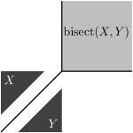
Figure 4: A bisector may be fat in the plane with the $\ell_{1}$ metric. Every point in the shaded region is at the same distance from $X$ and $Y$. The equation in Lemma 6 does not hold.

We note that the assumption on the considered metric in this lemma is necessary: As Figure 4 illustrates, the claim is not valid with the $\ell_{1}$ norm.

Proof of Lemma 6.

We have $\operatorname{dom}(Y,X)\supseteq\overline{\mathbb{R}^{d}\setminus\operatorname{dom}(X,Y)}$ because $\operatorname{dom}(Y,X)$ is closed and $\operatorname{dom}(Y,X)\cup\operatorname{dom}(X,Y)=\mathbb{R}^{d}$. For the other inclusion, let $z\in\operatorname{dom}(Y,X)$ and let $y$ be a closest point in $Y$ to $z$. Since $X$ does not intersect the open ball with centre $z$ and radius $\mathrm{dist}(y,z)$, any point $z^{\prime}\neq z$ on the segment $zy$ is strictly closer to $y$ than to $X$ (Figure 5), and thus is not in $\operatorname{dom}(X,Y)$. Since $z^{\prime}$ can be arbitrarily close to $z$, we have $z\in\overline{\mathbb{R}^{d}\setminus\operatorname{dom}(X,Y)}$.

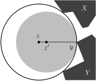
Figure 5: Since $X$ does not intersect the interior of the ball around $z$, it does not touch the ball around $z^{\prime}$.

∎

Lemma 7.

If $(R^{\infty}_{i},S^{\infty}_{i})_{i}$ is as in Proposition 5, then $\overline{R^{\infty}_{i}}\cap S^{\infty}_{j}=\emptyset$ whenever $0\leq i<j\leq k$.

Proof.

For contradiction, suppose that there is some $a\in\overline{R^{\infty}_{i}}\cap S^{\infty}_{j}$.

If $i>0$, then for each $n\in\mathbb{N}$ we have $a\in S^{\infty}_{j}\subseteq S^{n}_{j}\subseteq S^{n}_{i+1}$, so $\operatorname{dom}(R^{n}_{i-1},\{a\})\supseteq\operatorname{dom}(R^{n}_{i-1},S^{n}_{i+1})=R^{n+1}_{i}$. This implies $\mathrm{dist}(a,R^{n}_{i-1})\leq 2\cdot\mathrm{dist}(a,R^{n+1}_{i})$. Since $a\in\overline{R^{\infty}_{i}}$, the right-hand side tends to $0$ as $n\to\infty$, and hence, so does $\mathrm{dist}(a,R^{n}_{i-1})$. Thus, $a\in\overline{R^{\infty}_{i-1}}$. Repeating the same argument for $i-1$, $i-2$, …, we arrive at $a\in\overline{R^{\infty}_{0}}=P$.

Similarly, if $j<k$, then $a\in S^{\infty}_{j}\subseteq S^{n+1}_{j}=\operatorname{dom}(S^{n}_{j+1},R^{n}_{j-1})$ for all $n\in\mathbb{N}$. Thus, $\mathrm{dist}(a,S^{n}_{j+1})\leq\mathrm{dist}(a,R^{n}_{j-1})\leq\mathrm{dist}(a,R^{n}_{i})\to 0$ as $n\to\infty$ because $a\in\overline{R^{\infty}_{i}}$. So $a\in S^{\infty}_{j+1}$. Repeating the argument for $j+1$, $j+2$, …, we obtain $a\in S^{\infty}_{k}=Q$.

Thus we have $a\in P\cap Q$, contradicting the assumption that $P$ and $Q$ are disjoint. ∎

Proof of Proposition 5..

Our goal is to show that $F((\overline{R^{\infty}_{i}},S^{\infty}_{i})_{i})=(\overline{R^{\infty}_{i}},S^{\infty}_{i})_{i}$. Since $F$ is monotone, $F((\overline{R^{\infty}_{i}},S^{\infty}_{i})_{i})\geq F((R^{n}_{i},S^{n}_{i})_{i})\geq(R^{n}_{i},S^{n}_{i})_{i}$ for each $n$, and hence $F((\overline{R^{\infty}_{i}},S^{\infty}_{i})_{i})\geq(\overline{R^{\infty}_{i}},S^{\infty}_{i})_{i}$. It remains to show that $F((\overline{R^{\infty}_{i}},S^{\infty}_{i})_{i})\leq(\overline{R^{\infty}_{i}},S^{\infty}_{i})_{i}$, which means, by the definition of $F$, that

$$\operatorname{dom}(S^{\infty}_{i+1},\overline{R^{\infty}_{i-1}})\supseteq S^{\infty}_{i},$$ (13)

and

$$\operatorname{dom}(\overline{R^{\infty}_{i-1}},S^{\infty}_{i+1})\subseteq\overline{R^{\infty}_{i}}.$$ (14)

The inclusion (13) follows just by continuity of the distance function: We have $S^{\infty}_{i}=\bigcap_{n\in\mathbb{N}}S^{n+1}_{i}=\bigcap_{n\in\mathbb{N}}\operatorname{dom}\bigl{(}S^{n}_{i+1},R^{n}_{i-1}\bigr{)}$. So for $x\in S^{\infty}_{i}$ we have $\mathrm{dist}(x,S^{n}_{i+1})\leq\mathrm{dist}(x,R^{n}_{i-1})$ for every $n$, and $\mathrm{dist}(x,S^{\infty}_{i+1})=\lim_{n\to\infty}\mathrm{dist}(x,S^{n}_{i+1})\leq\lim_{n\to\infty}\mathrm{dist}(x,R^{n}_{i-1})=\mathrm{dist}(x,\overline{R^{\infty}_{i-1}})$. Hence $x\in\operatorname{dom}(S^{\infty}_{i+1},\overline{R^{\infty}_{i-1}})$ and (13) is proved.

For proving (14), we need the previous lemmas. By (13), we have

$$\mathbb{R}^{d}\setminus\operatorname{dom}(S^{\infty}_{i+1},\overline{R^{\infty}_{i-1}})\subseteq\mathbb{R}^{d}\setminus S^{\infty}_{i}\subseteq R^{\infty}_{i},$$ (15)

where the latter inclusion is because $R^{n}_{i}\cup S^{n}_{i}=\mathbb{R}^{d}$ for every $n$ (this was part of the definition of $\mathcal{L}$). We obtain (14) by taking the closure of (15), using Lemma 6 for the left-hand side; for applying this lemma, we need $\overline{R^{\infty}_{i-1}}\cap S^{\infty}_{i+1}=\emptyset$, which holds by Lemma 7. ∎

If the initial element $(R^{0}_{i},S^{0}_{i})_{i}$ in Proposition 5 is less than or equal to all $k$-gradations (with respect to the ordering $\mathord{\leq}$), then so is $(R^{n}_{i},S^{n}_{i})_{i}$ for all $n$ (inductively by the monotonicity of $F$), and therefore, the resulting $(\overline{R^{\infty}_{i}},S^{\infty}_{i})_{i}$ is the least $k$-gradation. This is the case when, for example, $(R^{0}_{i},S^{0}_{i})_{i}$ is the least element $(P,\mathbb{R}^{d})_{i}$ of $\mathcal{L}$.

The trisector in Figure 3 corresponds to the least $3$-gradation, but this $3$-gradation is not obtained by iteration from the least element of $\mathcal{L}$. This witnesses that Proposition 5 may indeed fail for norms that are not strictly convex.

Computational issues

Proposition 5 gives a method to draw a $k$-sector in Euclidean spaces: By applying $F$ iteratively, we get an ascending chain $(R^{0}_{i},S^{0}_{i})_{i}\leq(R^{1}_{i},S^{1}_{i})_{i}\leq\cdots$ whose supremum $(R^{\infty}_{i},S^{\infty}_{i})_{i}$ gives a $k$-gradation $(\overline{R^{\infty}_{i}},S^{\infty}_{i})_{i}$. If we stop the iteration after sufficiently many steps, we obtain an approximation of $(\overline{R^{\infty}_{i}},S^{\infty}_{i})_{i}$.

However, implementing the algorithm is not entirely trivial, because even if the sites are simple, applying $F$ repeatedly gives rise to regions that are hard to describe. For example, consider the case where $P$ and $Q$ are points in the plane, and we begin with $(R^{0}_{i},S^{0}_{i})_{i}=(P,\mathbb{R}^{2})_{i}$. Then $\partial R^{1}_{k-1}$ is the line bisecting $P$ and $Q$, and $\partial R^{2}_{k-2}$ is the parabola bisecting $P$ and this line. The next iteration yields the curve $\partial R^{3}_{k-3}$ (or $\partial R^{3}_{k-1}$) which bisects between a parabola and a point.

Thus, unlike typical basic operations allowed in computational geometry, taking the bisector gives rise to increasingly complicated curves. If we have an analytic description of the boundary curves of the regions $R^{n}_{i}$ and $S^{n}_{i}$, each of the curves defining $R^{n+1}_{i}$ and $S^{n+1}_{i}$ is described by a system of differential equations associated with the bisecting condition. But solving such equations exactly in each iterative step is computationally expensive. Therefore, we need to find a practical method for approximating the bisectors (assuming that we only compute the regions in a bounded area).

One method is to approximate each region by a polygonal region. We start with some polygonal approximations $\tilde{P}$, $\tilde{Q}$ of $P$, $Q$, and let $(\tilde{R}^{0}_{i},\tilde{S}^{0}_{i})_{i}:=(\tilde{P},\mathbb{R}^{d})_{i}$. Then for each $n$, we compute an approximation $(\tilde{R}^{n+1}_{i},\tilde{S}^{n+1}_{i})_{i}$ to $F((\tilde{R}^{n}_{i},\tilde{S}^{n}_{i})_{i})$, where the bisector of two polygonal regions, which is a piecewise quadratic curve, is approximated by a suitable polygonal region. To ensure that $(\tilde{R}^{n}_{i},\tilde{S}^{n}_{i})_{i}$ converges to an underestimate (with respect to the ordering $\leq$) of the least $k$-gradation $(\overline{R^{\infty}_{i}},S^{\infty}_{i})_{i}$, we should have $(\tilde{R}^{n}_{i},\tilde{S}^{n}_{i})_{i}\leq(\tilde{R}^{n+1}_{i},\tilde{S}^{n+1}_{i})_{i}\leq F((\tilde{R}^{n}_{i},\tilde{S}^{n}_{i})_{i})$. This can be achieved by computing an inner approximation of $R_{i}^{n+1}$ and an outer approximation of $S_{i}^{n+1}$.

Another method is to consider the problem in the pixel geometry, where each of the approximate regions $\tilde{R}^{n}_{i}$, $\tilde{S}^{n}_{i}$ is a set of pixels. In computing $(\tilde{R}^{n+1}_{i},\tilde{S}^{n+1}_{i})_{i}$, we again make sure that $(\tilde{R}^{n}_{i},\tilde{S}^{n}_{i})_{i}\leq(\tilde{R}^{n+1}_{i},\tilde{S}^{n+1}_{i})_{i}\leq F((\tilde{R}^{n}_{i},\tilde{S}^{n}_{i})_{i})$. Then $(\tilde{R}^{n}_{i},\tilde{S}^{n}_{i})_{i}$ stabilizes eventually, providing a lower estimate of the least $k$-gradation. The analysis of time complexity (as a function of precision) of these methods is left as a future research problem.

Uniqueness

The curves in Figure 1 were drawn using the pixel geometry model explained above. As we mentioned there, they are guaranteed to lie on $P$’s side of any true $k$-sector curves. By exchanging $P$ and $Q$, we obtain also an approximate $k$-sector that lies on $Q$’s side of any true $k$-sector. We tried computing these lower and upper estimates for several different $P$, $Q$ and $k$ in Euclidean plane, but we did not find them differ by a significant amount. Because of this, we suspect that the $k$-sector is always unique:

Conjecture.

The $k$-sector of any two disjoint nonempty closed sets in Euclidean space is unique.

Acknowledgements

We gratefully acknowledge valuable discussions with many friends including Tetsuo Asano and Günter Rote; indeed, we owe Tetsuo for precious information of his recent work on convex distance cases. We also thank Yu Muramatsu for his programming work in drawing figures. D. R. would like to express his thanks to Simeon Reich for his helpful discussion. Finally, we remark that the warm comments from the audience of the preliminary announcement at EuroCG 2009 encouraged us to work further on the subject.

A. K. is supported by the Nakajima Foundation and the Natural Sciences and Engineering Research Council of Canada. The part of this research by T. T. was partially supported by the JSPS Grant-in-Aid for Scientific Research (B) 18300001.

References

- [1] T. Asano and D. Kirkpatrick. Distance trisector curves in regular convex distance metrics. In Proceedings of the 3rd International Symposium on Voronoi Diagrams in Science and Engineering (ISVD 2006), July 2–5, Banff, Alberta, Canada, pp. 8–17.
- [2] T. Asano, J. Matoušek, and T. Tokuyama. Zone diagrams: Existence, uniqueness, and algorithmic challenge. SIAM Journal on Computing, 37(4):1182–1198, 2007.
- [3] T. Asano, J. Matoušek, and T. Tokuyama. The distance trisector curve. Advances in Mathematics, 212(1):338–360, 2007.
- [4] J. Chun, Y. Okada, and T. Tokuyama. Distance trisector of segments and zone diagram of segments in a plane. In Proceedings of the 4th International Symposium on Voronoi Diagrams in Science and Engineering (ISVD 2007), July 9–12, Pontypridd, Wales, UK, pp. 66–73.
- [5] K. Imai, A. Kawamura, J. Matoušek, Y. Muramatsu, and T. Tokuyama. Distance -sectors and zone diagrams. In Proceedings of the 25th European Workshop on Computational Geometry (EuroCG 2009), pp. 191–194.
- [6] A. Kawamura, J. Matoušek, and T. Tokuyama. Zone diagrams in Euclidean spaces and in other normed spaces. Preprint, arXiv:0912.3016v1.
- [7] D. Reem and S. Reich. Zone and double zone diagrams in abstract spaces. Colloquium Mathematicum, 115(1):129–145, 2009.
- [8] D. Reem. Voronoi and zone diagrams. PhD Thesis, Technion, Haifa, submitted September 2009.
- [9] A. Tarski. A lattice-theoretical fixpoint theorem and its applications. Pacific Journal of Mathematics, 5:285–309, 1955.