Statistical and coherence properties of radiation from X-ray free electron lasers

Abstract

We describe statistical and coherence properties of the radiation from x-ray free electron lasers (XFEL). It is shown that the X-ray FEL radiation before saturation is described with gaussian statistics. Particularly important is the case of the optimized X-ray FEL, studied in detail. Applying similarity techniques to the results of numerical simulations allowed us to find universal scaling relations for the main characteristics of an X-ray FEL operating in the saturation regime: efficiency, coherence time and degree of transverse coherence. We find that with an appropriate normalization of these quantities, they are functions of only the ratio of the geometrical emittance of the electron beam to the radiation wavelength. Statistical and coherence properties of the higher harmonics of the radiation are highlighted as well.

1 Introduction

Single pass free electron laser (FEL) amplifiers starting from shot noise in the electron beam have been intensively developed during the last decades. An origin for this development was an idea born in the early eighties to extend the operating wavelength range of FELs to the vacuum ultraviolet (VUV) and x-ray bands [1, 2, 3]. Significant efforts have been invested into the development of high brightness injectors, beam formation systems, linear accelerators, and undulators. The result was rapid extension of the wavelength range from infrared to hard x-rays [4, 5, 6, 7, 8, 9, 10, 11, 12, 13]. The first dedicated user facility FLASH at DESY in Hamburg is in operation since 2005 and provides wavelength range from 6.5 nm to 50 nm [14]. LCLS at Stanford has been recently commissioned and delivers radiation in the 0.15 nm - 1.5 nm wavelength range [13]. The two other dedicated facilities that are under construction at the moment, the European XFEL, and SCSS at Spring-8 [15, 16].

The high gain FEL amplifier starting from the shot noise in the electron beam is a very simple device. It is a system consisting of a relativistic electron beam and an undulator. The FEL collective instability in the electron beam produces an exponential growth (along the undulator) of the modulation of the electron density on the scale of undulator radiation wavelength. The initial seed for the amplification process are fluctuations of the electron beam current. Since shot noise in the electron beam is a stochastic process, the radiation produced by a SASE FEL possesses stochastic features as well. Its properties are naturally described in terms of statistical optics using notions of probability density distribution functions of the fields and intensities, correlation functions, notions of coherence time, degree of coherence, etc.

Development of the theoretical description of the coherence properties of the radiation from SASE FEL has spanned more than twenty years (see [19, 20, 21, 22, 23, 24, 25, 26, 27, 28, 29, 30, 31, 32, 33, 34, 35, 36]. This subject is rather complicated, and it is worth mentioning that theoretical predictions agree well with recent experimental results [7, 8, 9, 10, 37, 38, 39, 40]. Some averaged output characteristics of SASE FEL in framework of the one-dimensional model have been obtained in [19, 20]. An approach for time-dependent numerical simulations of SASE FEL has been developed in [21, 22]. Realization of this approach allowed one to obtain some statistical properties of the radiation from a SASE FEL operating in linear and nonlinear regime [23, 24]. A comprehensive study of the statistical properties of the radiation from the SASE FEL in the framework of the same model is presented in [25]. It has been shown that a SASE FEL operating in the linear regime is a completely chaotic polarized radiation source described with gaussian statistics. Short-pulse effects (for pulse durations comparable with the coherence time) have been studied in [22, 26, 27]. An important practical result was prediction of the significant suppression of the fluctuations of the radiation intensity after a narrow-band monochromator for the case of SASE FEL operation in the saturation regime [26]. Statistical description of the chaotic evolution of the radiation from SASE FEL has been presented in [28, 29].

The first analytical studies of the problem of transverse coherence relate to the late eighties [30, 31]. Later on more detailed studies have been performed [32]. The problem of start-up from the shot noise has been studied analytically and numerically for the linear stage of amplification using an approach developed in [31]. It has been found that the process of formation of transverse coherence is more complicated than that given by a naive physical picture of transverse mode selection. Namely, in the case of perfect mode selection the degree of transverse coherence is defined by the interdependence of the longitudinal and transverse coherence. Comprehensive studies of the evolution of transverse coherence in the linear and nonlinear regime of SASE FEL operation have been performed in [33, 34, 35]. It has been found that the coherence time and the degree of transverse coherence reach maximum values in the end of the linear regime. Maximum brilliance of the radiation is achieved in the very beginning of the nonlinear regime which is also referred as a saturation point [34]. Output power of the SASE FEL grows continuously in the nonlinear regime, while the brilliance drops down after passing saturation point.

2 Operation of an FEL amplifier

A single-pass FEL amplifier starting from the shot noise in the electron beam seems similar to the well known undulator insertion device: in both cases radiation is produced during single pass of the electron beam through the undulator. To reveal principal differences, we first recall the properties of incoherent radiation. Radiation within the cone of half angle $\theta_{\mathrm{con}}=\sqrt{1+K^{2}}/(\gamma\sqrt{N_{\mathrm{w}}})$ has relative spectral bandwidth $\Delta\lambda/\lambda\simeq 1/N_{\mathrm{w}}$ near the resonance wavelength $\lambda=(\lambda_{\mathrm{w}}/2\gamma^{2})(1+K^{2})$. Here $\lambda_{\mathrm{w}}$ is the undulator period, $N_{\mathrm{w}}$ is the number of undulator periods, $\gamma$ is the relativistic factor, $K=e\lambda_{\mathrm{w}}H_{\mathrm{w}}/2\pi mc^{2}$ is the undulator parameter, $H_{\mathrm{w}}$ is the rms undulator field, and $m$ and $e$ are the electron mass and charge, respectively. Radiation energy emitted by a single electron in the central cone is $E_{\mathrm{e}}\simeq 4\pi^{2}e^{2}K^{2}A_{\mathrm{JJ}}^{2}/[\lambda(1+K^{2})]$. Here $A_{\mathrm{JJ}}=1$ and $A_{\mathrm{JJ}}=[J_{0}(Q)-J_{1}(Q)]$ for a helical and a planar undulator, respectively, $J_{n}(Q)$ is a Bessel function of $n$th order, and $Q=K^{2}/2/(1+K^{2})$. Wavepackets emitted by different electrons are not correlated, thus radiated power of the electron bunch with current $I$ is just the radiation energy from a single electron multiplied by the electron flux $I/e$:

$$W_{\mathrm{incoh}}\simeq\left[\frac{4\pi^{2}eI}{\lambda}\right]\left[\frac{K^{2}}{1+K^{2}}\right]A_{\mathrm{JJ}}^{2}\ .$$ (1)

In the free electron laser, electron beam density is modulated by the period of resonance wavelength $\lambda$. Let us consider a model case of an electron beam with the gaussian distribution of the current density with rms width $\sigma$, and an axial modulation $I(z)=I[1+a_{\mathrm{in}}\cos(2\pi z/\lambda)]$. Total power radiated by a modulated electron beam has been derived in [41]:

$$W_{\mathrm{coh}}=\left[\frac{\pi^{2}a^{2}_{\mathrm{in}}I^{2}}{2c}\right]\left[\frac{K^{2}}{1+K^{2}}\right]A^{2}_{\mathrm{JJ}}N_{\mathrm{w}}F(N)\ ,$$ (2)

where

$$F(N)=\frac{2}{\pi}\left[\arctan\left(\frac{1}{2N}\right)+N\ln\left(\frac{4N^{2}}{4N^{2}+1}\right)\right]\ ,$$ (3)

$N=k\sigma^{2}/L_{\mathrm{w}}$ is the Fresnel number, $k=2\pi/\lambda$, and $L_{\mathrm{w}}=N_{\mathrm{w}}\lambda_{\mathrm{w}}$ is the undulator length. In Fig. 1 we present the plot of the universal function $F(N)$. It exhibits a simple behavior in the limits of large and small values of Fresnel number: $F(N)\to 1/(2\pi N)$ for $N\to\infty$, and $F(N)\to 1$ for $N\to 0$.

Figure 1: Plot of the universal function F (N) given by eq. (3). Dashed curve shows an asymptote for a wide electron beam $F=1/(2\pi N)$.

Analysis of expressions (1) and (2) tells us that incoherent radiation power corresponds to the radiation power of the modulated electron beam with effective modulation amplitude of $a_{\mathrm{in}}\sim 1/\sqrt{N_{\mathrm{w}}I\lambda/(ec)}$. Note that $N_{\mathrm{w}}I\lambda/(ec)$ is the number of electrons on the slippage length $N_{\mathrm{w}}\lambda$. Now we have quantitative answer to the question: how much the FEL radiation power exceeds the power of incoherent undulator radiation? In the free electron laser an amplitude of the electron beam density modulation reaches values of about unity, and the ratio of the radiation powers (coherent to incoherent) is a factor of about the number of electrons per slippage length.

Enhancement of the beam modulation in the free electron laser occurs due to the radiation-induced collective instability. When an electron beam traverses an undulator, it emits radiation at the resonance wavelength. The electromagnetic wave is always faster than the electrons, and a resonant condition occurs such that the radiation slips a distance $\lambda$ relative to the electrons after one undulator period. The fields produced by the moving charges in one part of the electron bunch react to moving charges in another part of the bunch leading to a growing concentration of particles wherever a small perturbation starts to occur. Electron bunches with very small transverse emittance (of about radiation wavelength) and high peak current (of about a few kA) are needed for the operation of short wavelength FELs.

The description of high gain FEL amplification refers to the class of self-consistent problems for which the field equations and equations of motion must be solved simultaneously. Characteristics of the amplification process can be obtained with a combination of analytical techniques and simulations with time dependent FEL simulation codes (see [18, 36] and references therein). The amplification process in the SASE FEL is triggered by the shot noise in the electron beam, then it passes the stage of exponential growth (also called the high gain linear regime), and finally enters saturation stage when the beam density modulation approaches unity. In the linear high-gain limit the radiation emitted by the electron beam in the undulator can be represented as a set of self-reproduced beam radiation modes [42]:

$$\tilde{E}=\int\mathrm{d}\omega\exp[i\omega(z/c-t)]\times\sum\limits_{n,k}A_{nk}(\omega,z)\Phi_{nk}(r,\omega)\exp[\Lambda_{nk}(\omega)z+in\phi]$$ (4)

described by the eigenvalue $\Lambda_{nk}(\omega)$ and the field distribution eigenfunction $\Phi_{nk}(r,\omega)$. Here $\omega=2\pi c/\lambda$ is the frequency of the electromagnetic wave. At a sufficient undulator length the fundamental mode (having maximum real part of the eigenvalue) begins to be the main contribution to the total radiation power. From a practical point of view, it is important to find an absolute minimum of the gain length $L_{\mathrm{g}}=1/\mathop{\mathrm{Re}}(\Lambda_{00})$ corresponding to the optimum focusing beta function. In the case of negligible space charge and energy spread effects (which is true for XFELs) the solution of the eigenvalue equation for the field gain length of the fundamental mode $L_{\mathrm{g}}$ and optimum beta function $\beta_{\mathrm{opt}}$ are well approximated by:

$$L_{\mathrm{g}} \simeq 1.67\left(\frac{I_{A}}{I}\right)^{1/2}\frac{(\epsilon_{n}\lambda_{\mathrm{w}})^{5/6}}{\lambda^{2/3}}\ \frac{(1+K^{2})^{1/3}}{KA_{JJ}}\ ,$$

$$\beta_{\mathrm{opt}} \simeq 11.2\left(\frac{I_{A}}{I}\right)^{1/2}\frac{\epsilon_{n}^{3/2}\lambda_{\mathrm{w}}^{1/2}}{\lambda KA_{JJ}}\ .$$ (5)

Here $\epsilon_{\mathrm{n}}$ is normalized emittance, and $I_{A}=mc^{3}/e\simeq 17$ kA is Alfven’s current. Dimensionless FEL equations are normalized using the gain parameter $\Gamma$ and the efficiency parameter $\bar{\rho}$ [18]:

$$\Gamma = \left[\frac{I}{I_{\mathrm{A}}}\frac{8\pi^{2}K^{2}A_{\mathrm{JJ}}^{2}}{\lambda\lambda_{\mathrm{w}}\gamma^{3}}\right]^{1/2}\ ,$$

$$\bar{\rho} = \frac{\lambda_{\mathrm{w}}\Gamma}{4\pi}\ .$$ (6)

Analysis of the dimensionless FEL equations tells us that the physical parameters describing operation of the optimized FEL (5), the diffraction parameter $B$ and the parameter of betatron oscillations $\hat{k}_{\beta}$, are only functions of the parameter $\hat{\epsilon}=2\pi\epsilon/\lambda$[18, 34, 44]:

$$B = 2\Gamma\sigma^{2}\omega/c\simeq 12.5\times\hat{\epsilon}^{5/2}\ ,$$

$$\hat{k}_{\beta} = 1/(\beta\Gamma)\simeq 0.158\times\hat{\epsilon}^{-3/2}\ .$$ (7)

Note that Eqs. (5) and (7) are accurate in the range $1<\hat{\epsilon}<5$.

The diffraction parameter $B$ directly relates to diffraction effects and the formation of transverse coherence. If diffraction expansion of the radiation on a scale of the field gain length is comparable with the transverse size of the electron beam, we can expect a high degree of transverse coherence. For this range of parameters the value of the diffraction parameter is small. If diffraction expansion of the radiation is small (which happens at large values of the diffraction parameter) then we can expect significant degradation in the degree of transverse coherence. This effect occurs simply because different parts of the beam produce radiation nearly independently. In terms of the radiation expansion in the eigenmodes (4) this range of parameters corresponds to the degeneration of modes [18]. Diffraction parameter for an optimized XFEL exhibits strong dependence on the parameter $\hat{\epsilon}$ (see eq. (7)), and we can expect that the degree of transverse coherence should drop rapidly with the increase of the parameter $\hat{\epsilon}$.

3 Definitions of the statistical properties of radiation

We describe radiation fields generated by a SASE FEL in terms of statistical optics [46]. Longitudinal and transverse coherence are described in terms of correlation functions. The first order time correlation function, $g_{1}(t,t^{\prime})$, is defined as:

$$g_{1}(\vec{r},t-t^{\prime})=\frac{\langle\tilde{E}(\vec{r},t)\tilde{E}^{*}(\vec{r},t^{\prime})\rangle}{\left[\langle\mid\tilde{E}(\vec{r},t)\mid^{2}\rangle\langle\mid\tilde{E}(\vec{r},t^{\prime})\mid^{2}\rangle\right]^{1/2}}\ .$$ (8)

For a stationary random process the time correlation functions are dependent on only one variable, $\tau=t-t^{\prime}$. The coherence time is defined as [47, 18]:

$$\tau_{\mathrm{c}}=\int\limits^{\infty}_{-\infty}|g_{1}(\tau)|^{2}\mathop{\mathrm{d}}\tau\ .$$ (9)

The transverse coherence properties of the radiation are described in terms of the transverse correlation functions. The first-order transverse correlation function is defined as

$$\gamma_{1}(\vec{r}_{\perp},\vec{r}\prime_{\perp},z,t)=\frac{\langle\tilde{E}(\vec{r}_{\perp},z,t)\tilde{E}^{*}(\vec{r}\prime_{\perp},z,t)\rangle}{\left[\langle|\tilde{E}(\vec{r}_{\perp},z,t)|^{2}\rangle\langle|\tilde{E}(\vec{r}\prime_{\perp},z,t)|^{2}\rangle\right]^{1/2}}\ ,$$

where $\tilde{E}$ is the slowly varying amplitude of the amplified wave, $E=\tilde{E}(\vec{r}_{\perp},z,t)\mathop{\mathrm{e}}^{\mathop{\mathrm{i}}\omega_{0}(z/c-t)}+{\mathrm{C.C.}}$ We consider the model of a stationary random process, meaning that $\gamma_{1}$ does not depend on time. Following ref. [34], we define the degree of transverse coherence as:

$$\zeta=\frac{\int|\gamma_{1}(\vec{r}_{\perp},\vec{r}\prime_{\perp})|^{2}I(\vec{r}_{\perp})I(\vec{r}\prime_{\perp})\mathop{\mathrm{d}}\vec{r}_{\perp}\mathop{\mathrm{d}}\vec{r}\prime_{\perp}}{[\int I(\vec{r}_{\perp})\mathop{\mathrm{d}}\vec{r}_{\perp}]^{2}}\ ,$$ (10)

where $I\propto|\tilde{E}|^{2}$ is the radiation intensity.

An important figure of merit of the radiation source is the degeneracy parameter $\delta$, the number of photons per mode (coherent state). Note that when $\delta\gg 1$, classical statistics are applicable, while a quantum description of the field is necessary as soon as $\delta$ is comparable to (or less than) one. Using the definitions of the coherence time (9) and of the degree of transverse coherence (10) we define the degeneracy parameter as

$$\delta=\dot{N}_{ph}\tau_{\mathrm{c}}\zeta\ ,$$ (11)

where $\dot{N}_{ph}$ is the photon flux. Peak brilliance of the radiation from an undulator is defined as a transversely coherent spectral flux:

$$B_{r}=\frac{\omega\mathop{\mathrm{d}}\dot{N}_{ph}}{\mathop{\mathrm{d}}\omega}\ \frac{\zeta}{\left(\lambda/2\right)^{2}}=\frac{4\sqrt{2}c\delta}{\lambda^{3}}\ .$$ (12)

When deriving right-hand term of the equation we used the fact that the spectrum shape of SASE FEL radiation in a high-gain linear regime and near saturation is close to Gaussian [18]. In this case the rms spectrum bandwidth $\sigma_{\omega}$ and coherence time obey the equation $\tau_{\mathrm{c}}=\sqrt{\pi}/\sigma_{\omega}$.

4 Probability distributions of the radiation fields and intensities

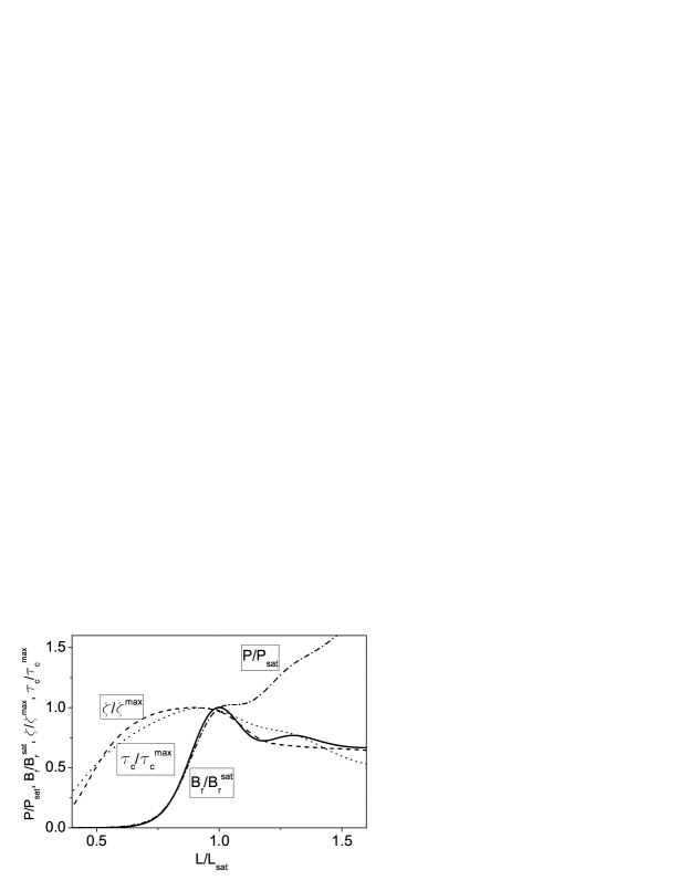
Figure 2: Evolution of main characteristics of SASE FEL along the undulator: brilliance (solid line), radiation power (dash-dotted line), degree of transverse coherence (dashed line), and coherence time (dotted line). Brilliance and radiation power are normalized to saturation values. Coherence time and degree of transverse coherence are normalized to the maximum values. Undulator length is normalized to saturation length. The plot has been derived from the parameter set corresponding to $\hat{\epsilon}=1$. Calculations have been performed with the simulation code FAST [48].

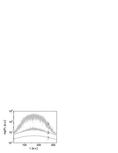
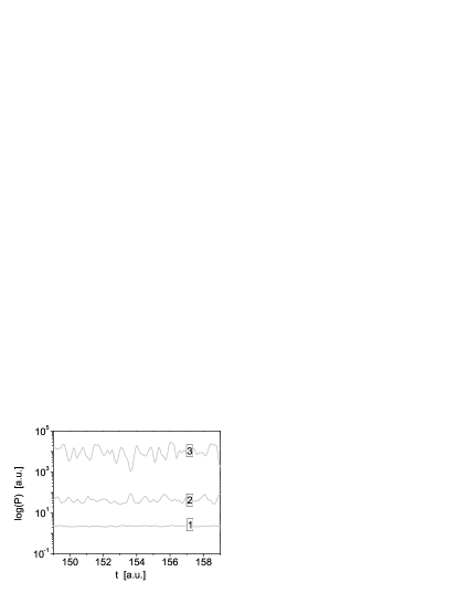
Figure 3: Temporal structure of the radiation pulse at different undulator lengths. Indexes 1, 2, and 3 correspond to the undulator length of $0.5L_{\mathrm{g}}$, $5L_{\mathrm{g}}$, and $10L_{\mathrm{g}}$, respectively. The plot in the right column represents the enlarged fraction of the plot in the left column. Calculations have been performed with the simulation code FAST [48].

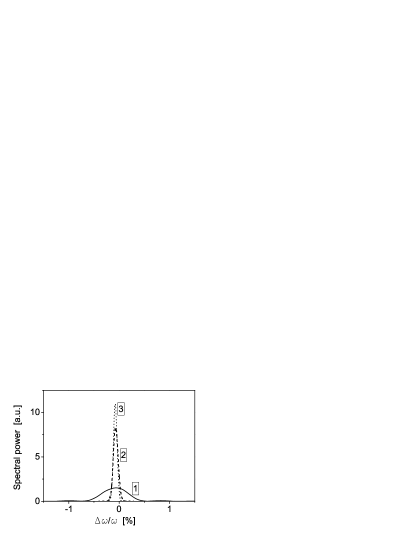
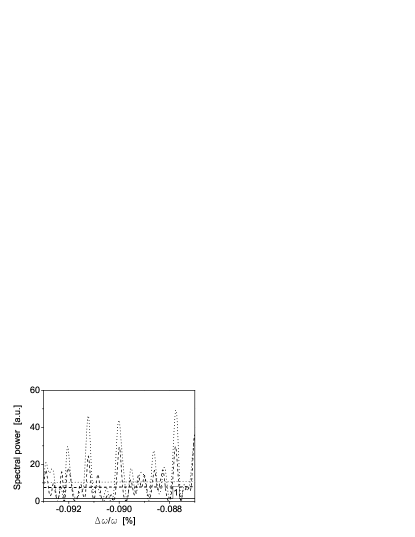
Figure 4: Spectral structure of the radiation pulse at different undulator length. Solid, dashed, and dotted line correspond to the undulator length of $0.5L_{\mathrm{g}}$, $5L_{\mathrm{g}}$, and $10L_{\mathrm{g}}$, respectively. The plot on the left-hand side shows only the envelope of the radiation spectrum. The plot on the right-hand side represents an enlarged fraction of the radiation spectrum. Calculations have been performed with the simulation code FAST [48].

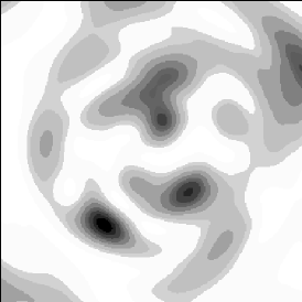
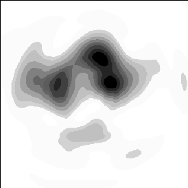
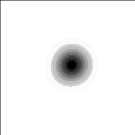
Figure 5: Snapshots of the power density distribution in a slice at the undulator length of $0.5L_{\mathrm{g}}$ (left plot), $5L_{\mathrm{g}}$ (middle plot), and $10L_{\mathrm{g}}$ (right plot). Calculations have been performed with the simulation code FAST [48].

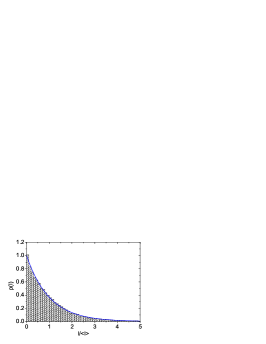
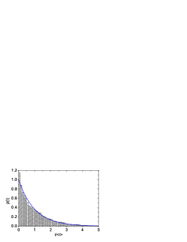
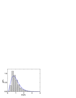
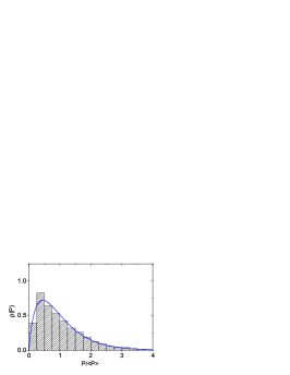
Figure 6: Probability density distributions of the instantaneous power density $I=|\tilde{E}|^{2}$ (top), and of the instantaneous radiation power $P$ (bottom) from a SASE FEL at different stages of amplification: linear regime, saturation regime, and deep nonlinear regime (undulator length of $5L_{\mathrm{g}}$, $10L_{\mathrm{g}}$, and $15L_{\mathrm{g}}$, respectively). Solid lines on the power density histograms (top) represent negative exponential distribution (14). Solid lines on power histograms (bottom) represent gamma distribution (15) with $M=1/\sigma_{\mathrm{P}}^{2}$. Here $\hat{\epsilon}=2$. Calculations have been performed with the simulation code FAST [48].

The amplification process in the SASE FEL starts from the shot noise in the electron beam, then it passes the stage of exponential amplification (high gain linear stage), and finally enters saturation stage (see Fig. 2). The field gain length of the fundamental radiation mode in the high gain linear regime is given by eq. (5), and saturation is achieved at the undulator length of about $L_{\mathrm{sat}}\simeq 10\times L_{\mathrm{g}}$ for the parameter space of modern X-ray FELs. Figures 3 and 4 show evolution of temporal and spectral structure of the radiation pulse along the undulator: at $0.5L_{\mathrm{g}}$ (beginning of the undulator), $5L_{\mathrm{g}}$ (high gain linear regime), and $10L_{\mathrm{g}}$ (saturation regime). Figure 5 shows snapshots of the intensity distributions across a slice of the photon pulse. We see that many transverse radiation modes are excited when the electron beam enters the undulator. Radiation field generated by SASE FEL consists of wavepackets (spikes [22]) which originate from fluctuations of the electron beam density. The typical length of a spike is about coherence length. Spectrum of the SASE FEL radiation also exhibits a spiky structure. The spectrum width is inversely proportional to the coherence time, and a typical width of a spike in a spectrum is inversely proportional to the pulse duration. The amplification process selects a narrow band of the radiation, the coherence time increases, and spectrum shrinks. Transverse coherence is also improved due to the mode selection process (4).

Figure 6 shows the probability distributions of the instantaneous power density $I\propto|\tilde{E}|^{2}$ (plots on top), and of the instantaneous radiation power $P\propto\int I(\vec{r}_{\perp})\mathop{\mathrm{d}}\vec{r}_{\perp}$ (plots on bottom). We see that transverse and longitudinal distributions of the radiation intensity exhibit rather chaotic behavior. On the other hand, probability distributions of the instantaneous power density $I$ and of the instantaneous radiation power $P$ look more elegant and seem to be described by simple functions. The origin of this fundamental simplicity relates to the properties of the electron beam. The shot noise in the electron beam has a statistical nature that significantly influences characteristics of the output radiation from a SASE FEL. Fluctuations of the electron beam current density serve as input signals in a SASE FEL. These fluctuations always exist in the electron beam due to the effect of shot noise. Initially fluctuations are not correlated in space and time, but when the electron beam enters the undulator, beam modulation at frequencies close to the resonance frequency of the FEL amplifier initiates the process of the amplification of coherent radiation.

Let us consider microscopic picture of the electron beam current at the entrance of the undulator. The electron beam current consists of moving electrons randomly arriving at the entrance of the undulator:

$$I(t)=(-e)\sum_{k=1}^{N}\delta(t-t_{k})\ ,$$

where $\delta(\ldots)$ is delta-function, (-e) is the charge of the electron, $N$ is the number of electrons in a bunch and $t_{k}$ is the random arrival time of the electron to the undulator entrance. The electron beam current $I(t)$ and its Fourier transform $\bar{I}(\omega)$ are connected by Fourier transformations :

$$I(t) = (-e)\sum_{k=1}^{N}\delta(t-t_{k})=\frac{1}{2\pi}\int\limits_{-\infty}^{\infty}\bar{I}(\omega)e^{-i\omega t}d\omega\ ,$$

$$\bar{I}(\omega) = \int\limits_{-\infty}^{\infty}e^{i\omega t}I(t)dt=(-e)\sum_{k=1}^{N}e^{i\omega t_{k}}\ .$$ (13)

It follows from eq. (13) that the Fourier transformation of the input current, $\bar{I}(\omega)$, is the sum of large number of complex phasors with random phases $\phi_{k}=\omega t_{k}$. Thus, harmonics of the electron beam current are described with gaussian statistics.

The FEL process is just an amplification of the initial shot noise in the narrow band near the resonance wavelength $\lambda$ when both harmonics of the beam current and radiation are growing. An FEL amplifier operating in the linear regime is just a linear filter, and the Fourier harmonic of the radiation field is simply proportional to the Fourier harmonic of the electron beam current, $\bar{E}(\omega)=H_{A}(\omega-\omega_{0})\bar{I}(\omega)$. Thus, the statistics of the radiation are gaussian – the same as of the shot noise in the electron beam. This kind of radiation is usually referred to as completely chaotic polarized light, a well known object in the field of statistical optics [46]. For instance, the higher order correlation functions (time and spectral) are expressed via the first order correlation function. The spectral density of the radiation energy and the first-order time correlation function form a Fourier transform pair (Wiener Khintchine theorem). The real and imaginary parts of the slowly varying complex amplitudes of the electric field of the electromagnetic wave, $\tilde{E}$ , have a Gaussian distribution. The instantaneous power density, $I=|\tilde{E}|^{2}$, fluctuates in accordance with the negative exponential distribution (see Fig. 6):

$$p(I)=\frac{1}{\langle I\rangle}\exp\left(-\frac{I}{\langle I\rangle}\right)\ .$$ (14)

Any integral of the power density, like radiation power $P$, fluctuates in accordance with the gamma distribution:

$$p({P})=\frac{M^{M}}{\Gamma(M)}\left(\frac{P}{\langle P\rangle}\right)^{M-1}\frac{1}{\langle P\rangle}\exp\left(-M\frac{P}{\langle P\rangle}\right)\ ,$$ (15)

where $\Gamma(M)$ is the gamma function with argument $M=1/\sigma_{\mathrm{P}}^{2}$, and $\sigma_{\mathrm{P}}^{2}=\langle(P-\langle P\rangle)^{2}\rangle/\langle P\rangle^{2}$ is the relative dispersion of the radiation power. For completely chaotic polarized light parameter $M$ has a clear physical interpretation – it is the number of modes [18]. Thus, the relative dispersion of the radiation power directly relates to the coherence properties of the SASE FEL operating in the linear regime. The degree of transverse coherence in this case can be defined as [18]:

$$\zeta=\frac{1}{M}=\sigma^{2}_{\mathrm{P}}\ .$$ (16)

It is shown in ref. [34] that such a definition for the degree of transverse coherence is mathematically equivalent to (10).

When amplification process enters nonlinear stage and reaches saturation, statistics of the radiation significantly deviate from gaussian. Particular signature of this change is illustrated in Fig. 6. We see that the probability distribution of the radiation intensity is not the negative exponential, and the probability distribution of the radiation power visibly deviates from gamma distribution. Up to now there is no analytical description of the statistics in the saturation regime, and we refer the reader to the analysis of the results of numerical simulations [34]. General feature of the saturation regime is that fluctuations of the radiation intensity are significantly suppressed. We also find that the definition of the degree of transverse coherence (16) has no physical sense near the saturation point.

When we trace the amplification process further in the nonlinear regime, we obtain that fluctuations of the radiation intensity and radiation power increase, and relevant probability distributions tend to those given by eqs. (14) and (15). This behavior hints that the properties of the radiation from a SASE FEL operating in the deep nonlinear regime tend to be those of completely chaotic polarized light [25, 34]. For the deep nonlinear regime we find that the degree of transverse coherence defined by (10) again tends to be an agreement with (16).

Another practical problem refers to the probability distributions of the radiation intensity in the frequency domain, like that filtered by monochromator. For SASE FEL radiation produced in the linear regime the probability distribution radiation intensity is defined by gaussian statistics, and it is the negative exponential for a narrow band monochromator. When amplification process enters saturation regime, this property still holds for the case of long electron pulse [18, 25], and is violated significantly for the case of short electron bunch, of about or less than coherence length. In the latter case fluctuations of the radiation intensity after narrow band monochromator are significantly suppressed as it has been predicted theoretically and measured experimentally at the free electron laser FLASH at DESY operating in a femtosecond mode [26, 37].

All considerations presented above are related to the fundamental harmonic of the SASE FEL radiation. Radiation from a SASE FEL with a planar undulator has rich harmonics contents. Intensities of even harmonics are suppressed [49], but odd harmonics provide significant contribution to the total radiation power [50, 51, 52, 53, 54]. Comprehensive studies of the statistical properties of the odd harmonics have been performed in paper [45]. It has been found that the statistics of the high-harmonic radiation from the SASE FEL changes significantly with respect to the fundamental harmonic (with respect to gaussian statistics). For the fundamental harmonic the probability density function of the intensity is the negative exponential distribution: $p(W)=\langle{W}\rangle^{-1}\exp(-W/\langle{W}\rangle)$. Mechanism of the higher harmonic generation is equivalent to the transformation of the intensity $W$ as $z=(W)^{n}$, where $n$ is the harmonic number. It has been shown in [45] that the probability distribution for the intensity of the n-th harmonic is given by:

$$p(z)=\frac{z}{n\langle{W}\rangle}{z}^{(1-n)/n}\exp(-z^{1/n}/\langle{W}\rangle)\ .$$ (17)

The expression for the mean value is $\langle{z}\rangle=n!\langle{W}\rangle^{n}$. Thus, the $n$th-harmonic radiation for the SASE FEL has an intensity level roughly $n!$ times larger than the corresponding steady-state case, but with more shot-to-shot fluctuations compared to the fundamental [54]. Nontrivial behavior of the intensity of the high harmonic reflects the complicated nonlinear transformation of the fundamental harmonic statistics. In this case a gaussian statistics are no longer valid. Practically this behavior occurs only in the very end of high gain exponential regime when coherent radiation intensity exceeds an incoherent one. When amplification enters nonlinear stage, probability distributions change dramatically on a scale of the gain length, and already in the saturation regime (and further downstream the undulator) the probability distributions of the radiation intensity of higher harmonics are pretty much close to the negative exponential distribution [45].

5 Characteristics of the radiation from SASE FEL operating in the saturation regime

Figure 7: Degree of transverse coherence $\zeta_{\mathrm{sat}}$ in the saturation point versus parameter $\hat{\epsilon}$. The number of electrons in the coherence volume is $N_{\mathrm{c}}=4\times 10^{6}$. Calculations have been performed with the simulation code FAST [48].

In Fig. 2 we present evolution of the main characteristics of a SASE FEL along the undulator. If one traces evolution of the brilliance (degeneracy parameter) of the radiation along the undulator length, there is always the point (defined as the saturation point [34]) where the brilliance reaches maximum value. The best properties of the radiation in terms of transverse and longitudinal coherence are reached just before the saturation point, and then degrade significantly despite the radiation power continuing to grow with the undulator length.

Application of similarity techniques allows us to derive universal parametric dependencies of the output characteristics of the radiation at the saturation point. As we mentioned in Section 2, within accepted approximations (optimized SASE FEL and negligibly small energy spread in the electron beam), normalized output characteristics of a SASE FEL at the saturation point are functions of only two parameters: $\hat{\epsilon}=2\pi\epsilon/\lambda$ and the number of electrons in the volume of coherence $N_{\mathrm{c}}=IN_{\mathrm{g}}\lambda/c$, where $N_{\mathrm{g}}=L_{\mathrm{g}}/\lambda_{\mathrm{w}}$ is the number of undulator periods per gain length. Characteristics of practical interest are: saturation length $L_{\mathrm{sat}}$, saturation efficiency $\eta_{\mathrm{sat}}=P_{\mathrm{sat}}/P_{\mathrm{b}}$ (ratio of the radiation power to the electron beam power $P_{\mathrm{b}}=\gamma mc^{2}I/e$), coherence time $\tau_{\mathrm{c}}$, degree of transverse coherence $\zeta$, degeneracy parameter $\delta$, and brilliance $B_{\mathrm{r}}$. Applications of similarity techniques to the results of numerical simulations of a SASE FEL [34] gives us the following result:

$$\hat{L}_{\mathrm{sat}} = \Gamma L_{\mathrm{sat}}\simeq 2.5\times\hat{\epsilon}^{5/6}\times\ln N_{\mathrm{c}}\ ,$$

$$\hat{\eta} = P/(\bar{\rho}P_{\mathrm{b}})\simeq 0.17/\hat{\epsilon}\ ,$$

$$\hat{\tau_{\mathrm{c}}} = \bar{\rho}\omega\tau_{\mathrm{c}}\simeq 1.16\times\sqrt{\ln N_{\mathrm{c}}}\times\hat{\epsilon}^{5/6}\ ,$$

$$\sigma_{\omega} = \sqrt{\pi}/\tau_{\mathrm{c}}\ .$$ (18)

These expressions provide reasonable practical accuracy for $\hat{\epsilon}\gtrsim 0.5$. With logarithmic accuracy in terms of $N_{\mathrm{c}}$ characteristics of the SASE FEL expressed in a normalized form are functions of the only parameter $\hat{\epsilon}$. The saturation length, FEL efficiency, and coherence time exhibit monotonous behavior in the parameter space of modern XFELs ($\hat{\epsilon}\simeq 0.5\ldots 5$). Situation is a bit complicated with the degree of transverse coherence as one can see in Fig. 7. The degree of transverse coherence reaches a maximum value in the range of $\hat{\epsilon}\sim 1$, and drops at small and large values of $\hat{\epsilon}$. At small values of the emittance, the degree of transverse coherence is limited by the interdependence of poor longitudinal coherence and transverse coherence [32]. Due to the start-up from shot noise, every radiation mode entering eq. (4) is excited within finite spectral bandwidth. This means that the radiation from a SASE FEL is formed by many fundamental TEM₀₀ modes with different frequencies. The transverse distribution of the radiation field of the mode is also different for different frequencies. Smaller values of $\hat{\epsilon}$ (smaller value of the diffraction parameter) correspond to larger frequency bandwidths. This effect explains the decrease of the transverse coherence at small values of $\hat{\epsilon}$. The degree of transverse coherence asymptotically approaches unity as $(1-\zeta)\propto 1/z\propto 1/\ln N_{\mathrm{c}}$ at small values of the emittance.

In the case of large emittance the degree of transverse coherence is defined by the contents of higher transverse modes [34, 35]. When $\hat{\epsilon}$ increases, the diffraction parameter increases as well, leading to the degeneration of the radiation modes [18]. The amplification process in the SASE FEL passes limited number of the field gain lengths, and starting from some value of $\hat{\epsilon}$, the linear stage of amplification becomes too short to provide a mode selection process (4). When the amplification process enters the nonlinear stage, the mode content of the radiation becomes richer due to independent growth of the radiation modes in the nonlinear medium. Thus, at large values of $\hat{\epsilon}$ the degree of transverse coherence is limited by poor mode selection. The degree of transverse coherence scales as $\zeta_{\mathrm{sat}}\propto(\ln N_{\mathrm{c}}/\hat{\epsilon})^{2}$ in the asymptote of large emittance. To avoid complications, we present here just a fit for the degree of transverse coherence for the number of electrons in the coherence volume $N_{\mathrm{c}}=4\times 10^{6}$:

$$\zeta_{\mathrm{sat}}\simeq\frac{1.1\hat{\epsilon}^{1/4}}{1+0.15\hat{\epsilon}^{9/4}}\ .$$ (19)

Recalculation from reduced to dimensional parameters is straightforward. For instance, saturation length is $L_{\mathrm{sat}}\simeq 0.6\times L_{\mathrm{g}}\times\ln N_{\mathrm{c}}$. Using (18) and (19) we can calculate normalized degeneracy parameter $\hat{\delta}=\hat{\eta}\zeta\hat{\tau_{\mathrm{c}}}$ and then the brilliance (12):

$$B_{r}\left[\frac{\mathrm{photons}}{\mathrm{sec\ mrad^{2}\ mm^{2}\ 0.1\%\ bandw.)}}\right]\simeq 4.5\times 10^{31}\times\frac{I[\mathrm{kA}]\times E[\mathrm{GeV}]}{\lambda[\mathrm{\AA}\ ]}\times\hat{\delta}\ .$$ (20)

Properties of the odd harmonics of the radiation from a SASE FEL with a planar undulator operating in the saturation regime also possess simple features. In the case of cold electron beam contributions of the higher odd harmonics to the FEL power are functions of the only undulator parameter $K$ [45]:

$$\frac{\langle W_{3}\rangle}{\langle W_{1}\rangle}|_{\mathrm{sat}}=0.094\times\frac{K_{3}^{2}}{K_{1}^{2}}\ ,\qquad\frac{\langle W_{5}\rangle}{\langle W_{1}\rangle}|_{\mathrm{sat}}=0.03\times\frac{K_{5}^{2}}{K_{1}^{2}}\ .$$ (21)

Here $K_{h}=K(-1)^{(h-1)/2}[J_{(h-1)/2}(Q)-J_{(h+1)/2}(Q)]$, $Q=K^{2}/[2(1+K^{2})]$, and $h$ is an odd integer. Influence of the energy spread and emittance leads to significant decrease of the power of higher harmonics, up to a factor of three for the third harmonic, and a factor of up to ten for the fifth harmonic. Power of the higher harmonics is subjected to larger fluctuations than the power of the fundamental harmonic as we mentioned in the previous section. The coherence time at saturation scales inversely proportional to the harmonic number, while relative spectrum bandwidth remains constant with the harmonic number.

6 Estimations in the framework of the one-dimensional model

An estimation of SASE FEL characteristics is frequently performed in the framework of the one-dimensional model in terms of the FEL parameter $\rho$ [55]:

$$\rho=\frac{\lambda_{\mathrm{w}}}{4\pi}\left[\frac{4\pi^{2}j_{0}K^{2}A_{\mathrm{JJ}}^{2}}{I_{A}\lambda_{\mathrm{w}}\gamma^{3}}\right]^{1/3}\ ,$$ (22)

where $j_{0}=I/(2\pi\sigma^{2})$ is the beam current density, $\sigma=\sqrt{\beta\epsilon_{\mathrm{n}}/\gamma}$ is rms transverse size of the electron beam, and $\beta$ is external focusing beta function. FEL parameter $\rho$ relates to the efficiency parameter of the 3D FEL theory as $\rho=\bar{\rho}/B^{1/3}$. Basic characteristics of the SASE FEL are estimated in terms of the parameter $\rho$ and number of cooperating electrons $N_{\mathrm{c}}=I/(e\rho\omega)$. Here we present a set of simple formulae extracted from [18, 22, 25]:

$$\mathrm{The\ field\ gain\ length:}\quad L_{\mathrm{g}}\sim\frac{\lambda_{\mathrm{w}}}{4\pi\rho}\ ,$$

$$\mathrm{Saturation\ length:}\quad L_{\mathrm{sat}}\sim\frac{\lambda_{\mathrm{w}}}{4\pi\rho}\left[3+\frac{\ln N_{\mathrm{c}}}{\sqrt{3}}\right]$$

$$\mathrm{Effective\ power\ of\ shot\ noise:}\quad \frac{P_{\mathrm{sh}}}{\rho P_{\mathrm{b}}}\simeq\frac{3}{N_{\mathrm{c}}\sqrt{\pi\ln N_{\mathrm{c}}}}\ ,$$

$$\mathrm{Saturation\ efficiency:}\quad \rho\ ,$$

$$\mathrm{The\ power\ gain\ at\ saturation:}\quad G\simeq\frac{1}{3}N_{\mathrm{c}}\sqrt{\pi\ln N_{\mathrm{c}}}\ ,$$

$$\mathrm{Coherence\ time\ at\ saturation:}\quad \tau_{\mathrm{c}}\simeq\frac{1}{\rho\omega}\sqrt{\frac{\pi\ln N_{\mathrm{c}}}{18}}\ .$$

$$\mathrm{Spectrum\ bandwidth:}\quad \sigma_{\omega}=\sqrt{\pi}/\tau_{\mathrm{c}}\ ,$$ (23)

In many cases this set of formulas can help quickly estimate main parameters of a SASE FEL but it does not provide complete self-consistent basis for optimization of this device.

References

References

- [1] A.M. Kondratenko, E.L. Saldin, Sov. Phys. Dokl. vol. 24, No. 12 (1979)986; Part. Accelerators 10(1980)207.
- [2] Ya.S. Derbenev, A.M. Kondratenko, and E.L. Saldin, Nucl. Instrum. and Methods 193(1982)415.
- [3] J.B. Murphy and C. Pellegrini, Nucl. Instrum. and Methods A237(1985)159.
- [4] M. Hogan et al., Phys. Rev. Lett. 81(1998)4867.
- [5] S. V. Milton et al., Science, 292(2000)2037.
- [6] A. Tremaine et al., Nucl. Instrum. and Methods A483(2002)24.
- [7] V. Ayvazyan et al., Phys. Rev. Lett. 88(2002)104802.
- [8] V. Ayvazyan et al., Eur. Phys. J. D20(2002)149.
- [9] V. Ayvazyan et al., Eur. Phys. J. D 37(2006)297.
- [10] W. Ackermann et al., Nature Photonics 1(2007)336.
- [11] T. Shintake et al., Nature Photonics 2(2008)555.
- [12] P. Emma, ”First lasing of the LCLS X-ray FEL at 1.5 A”, presented at the Particle Accelerator Conf., Vancouver, May 2009.
- [13] P. Emma, Lasing and saturation of the LCLS FEL, Proc. FEL09 Conference, TUOA01.
- [14] K. Tiedtke et al., New Journal of Physics 11(2009)023029
- [15] SCSS X-FEL: Conceptual design report, RIKEN, Japan, May 2005. (see also http://www-xfel.spring8.or.jp).
- [16] M. Altarelli et al. (Eds.), XFEL: The European X-Ray Free-Electron Laser. Technical Design Report, Preprint DESY 2006-097, DESY, Hamburg, 2006 (see also http://xfel.desy.de).
- [17] R. Bonifacio, F. Casagrande and L. De Salvo Souza, Phys. Rev. A 33(1986)2836.
- [18] E.L. Saldin, E.A. Schneidmiller, M.V. Yurkov, “The Physics of Free Electron Lasers” (Springer-Verlag, Berlin, 1999).
- [19] K.J. Kim, Nucl. Instrum. and Methods A 250(1986)396.
- [20] J.M. Wang and L.H. Yu, Nucl. Instrum. and Methods A 250(1986)484.
- [21] W.B. Colson, Review in: W.B. Colson et al. (Eds), ”Laser Handbook, Vol.6: Free Electron Laser” (North-Holland, Amsterdam, 1990), p. 115.
- [22] R. Bonifacio, et al., Phys. Rev. Lett. 73(1994)70.
- [23] P. Pierini and W. Fawley, Nucl. Instrum. and Methods A 375(1996)332.
- [24] E. L. Saldin, E. A. Schneidmiller, and M. V. Yurkov, Nucl. Instrum. and Methods A 393(1997)157.
- [25] E. L. Saldin, E. A. Schneidmiller, and M. V. Yurkov, Opt. Commun. 148(1998)383.
- [26] E.L. Saldin, E.A. Schneidmiller, and M.V. Yurkov, Nucl. Instrum. and Methods A507(2003)101.
- [27] E.L. Saldin, E.A. Schneidmiller, and M.V. Yurkov, Nucl. Instrum. and Methods A562(2006)472.
- [28] S. Krinsky and R.L. Gluckstern, Phys. Rev. ST Accel. Beams 6(2003)050701.
- [29] S. Krinsky and Y. Li, Phys. Rev. E73 (2006)066501.
- [30] L.H. Yu and S. Krinsky, Nucl. Instrum. and Methods A 285 (1989)119.
- [31] S. Krinsky and L.H. Yu, Phys. Rev. A 35(1987)3406.
- [32] E.L. Saldin, E.A. Schneidmiller, and M.V. Yurkov, Opt. Commun. 186(2000)185.
- [33] E.L. Saldin, E.A. Schneidmiller, and M.V. Yurkov, Nucl. Instrum. and Methods A 507(2003)106.
- [34] E.L. Saldin, E.A. Schneidmiller, and M.V. Yurkov, Opt. Commun. 281(2008)1179.
- [35] E.L. Saldin, E.A. Schneidmiller, and M.V. Yurkov, Opt. Commun. 281(2008)4727.
- [36] Z. Huang and K.-J. Kim, Phys. Rev. ST Accel. Beams 10(2007)034801.
- [37] V. Ayvazyan et al., Nucl. Instrum. and Methods A507(2003)368.
- [38] R. Ischebeck et al., Nucl. Instrum. and Methods A507(2003)175.
- [39] Y. Li et al., Phys. Rev. Lett. 91(2003)243602.
- [40] Y. Li et al., Phys. Rev. B80(2004)31.
- [41] E.L. Saldin, E.A. Schneidmiller, and M.V. Yurkov, Nucl. Instrum. and Methods A539(2005)499.
- [42] G. Moore, Opt. Commun. 52(1984)46.
- [43] E.L. Saldin, E. A. Schneidmiller, and M.V. Yurkov, Opt. Commun. 235(2004)415.
- [44] E.L. Saldin, E.A. Schneidmiller and M.V. Yurkov, Nucl. Instrum. and Methods A475(2001)86.
- [45] E.L. Saldin, E.A. Schneidmiller and M.V. Yurkov, Phys. Rev. ST Accel. Beams 9(2006)030702.
- [46] J. Goodman, Statistical Optics, (John Wiley and Sons, New York, 1985).
- [47] L. Mandel, Proc. Phys. Soc. (London), 1959, v.74, p.223.
- [48] E.L. Saldin, E.A. Schneidmiller, and M.V. Yurkov, Nucl. Instrum. and Methods A 429(1999)233.
- [49] G. Geloni et al., Opt. Commun. 271(2007)207.
- [50] M. Schmitt and C. Elliot, Phys. Rev. A, 34(1986)6.
- [51] R. Bonifacio, L. De Salvo, and P. Pierini, Nucl. Instr. Meth. A293(1990)627.
- [52] W.M. Fawley, Proc. IEEE Part. Acc. Conf., 1995, p.219.
- [53] H. Freund, S. Biedron and S. Milton, Nucl. Instr. Meth. A 445(2000)53.
- [54] Z. Huang and K. Kim, Phys. Rev. E, 62(2000)7295.
- [55] R. Bonifacio, C. Pellegrini and L.M. Narducci, Opt. Commun. 50(1984)373.