Testing the Reliability of Cluster Mass Indicators with a Systematics Limited Dataset

Abstract

We present the mass–X-ray observable scaling relationships for clusters of galaxies using the XMM-Newton cluster catalog of Snowden et al.. Our results are roughly consistent with previous observational and theoretical work, with one major exception. We find 2–3 times the scatter around the best fit mass scaling relationships as expected from cluster simulations or seen in other observational studies. We suggest that this is a consequence of using hydrostatic mass, as opposed to virial mass, and is due to the explicit dependence of the hydrostatic mass on the gradients of the temperature and gas density profiles. We find a larger range of slope in the cluster temperature profiles at $r_{500}$ than previous observational studies. Additionally, we find only a weak dependence of the gas mass fraction on cluster mass, consistent with a constant. Our average gas mass fraction results argue for a closer study of the systematic errors due to instrumental calibration and analysis method variations. We suggest that a more careful study of the differences between various observational results and with cluster simulations is needed to understand sources of bias and scatter in cosmological studies of galaxy clusters.

1 Introduction

Studies of clusters of galaxies provide for a variety of cosmological tests (see Voit, 2005, for a recent review). The precision of these tests is limited by the accuracy and precision of the scaling relations used to transform X-ray observables, such as temperature or luminosity, into cluster mass measurements (e.g., Rapetti et al., 2008; Vikhlinin et al., 2009). Improved modeling of the complex physics at work in clusters has led to better study of the sources of bias and scatter in the mass scaling relationships. These models suggest that the hydrostatic equilibrium assumption used to calculate total cluster masses from X-ray data can lead to underestimates on the order of 10–20% (e.g., Nagai et al., 2007b). The discrepancy is explained by the presence of nonthermal pressure support in clusters. Theoretical studies have found that the expected scatter in mass scaling relationships is dependent on the dynamical state of the clusters under study (e.g., Kravtsov et al., 2006). Relaxed systems should show lower scatter around the best-fit relation than disturbed clusters.

This information can be used to tailor observational programs, particularly by limiting the bias and scatter in the mass scaling relationships. One suggestion is to use only relaxed clusters in cosmological studies. However for high redshift samples, relaxed clusters make up only a minority of the cluster population (see e.g., Vikhlinin et al., 2009). Alternatively, the right choice of mass proxy could provide low scatter data. Kravtsov et al. (2006) proposed a new X-ray proxy for cluster mass, the parameter $Y_{X}$ which is the product of X-ray temperature and gas mass. The $Y_{X}$ parameter is related to the total thermal energy of the cluster gas and is an X-ray analog to the Sunyaev-Zel’dovich (SZ) flux. From cluster simulations, Kravtsov et al. (2006) found that the scatter in the cluster mass–$Y_{X}$ scaling law is not only lower than for other commonly used mass proxies, but also shows little dependence on cluster dynamical state.

Observational studies of the $Y_{X}$ parameter as a mass proxy have been limited in the number of clusters used and the statistical quality of the data (Arnaud et al., 2007; Vikhlinin et al., 2009). The statistical error was on the order of the measured scatter, making it difficult to determine the intrinsic scatter in the relationship. Additionally, previous observational work has focused solely on a limited number of relaxed systems. A larger and more sensitive observational study of clusters will better test the $Y_{X}$ mass proxy and the results of cluster simulations. In this Letter, we use the data from a recent high signal-to-noise XMM-Newton survey of nearby clusters to test the usefulness of various mass proxies. We assume $H_{0}=70$ km s^-1 Mpc^-1, $\Omega_{M}=0.3$, and $\Omega_{\Lambda}=0.7$.

2 Data Analysis

Our cluster sample was taken from Snowden et al. (2008), which presented the projected temperature, abundance, and surface brightness profiles for 70 clusters found by fitting XMM-Newton data (see that work for details of the spectral analysis). While not an unbiased sample, the large number of clusters does provide a wide range of cluster properties to study. It is not limited to relaxed and/or hot ($>5$ keV) clusters. The selection criteria used by Snowden et al. (2008) excluded highly asymmetric clusters and those with strong substructure (e.g., A115, A754). However, some merging clusters were included in the sample (e.g., A520, the Bullet Cluster).

We used the projected profiles to determine the gas density and three-dimensional temperature profiles following the procedure of Vikhlinin et al. (2006). The same gas density and temperature models were used with some simplification. The lower spatial resolution of our data did not constrain the second $\beta$-model component required to fit the Chandra data in the cluster center, therefore we did not include it. We also compared fits with and without steepening at large radii and excluded the steepening when it did not produce a significantly better fit of the data. For the temperature fits, we took into account projection effects and used the spectral temperature weighting formalism of Vikhlinin (2006). When cooling in the core was not obvious we fixed the cool component parameters to produce a flat temperature profile in the center.

We calculated the total cluster mass distribution for each cluster assuming hydrostatic equilibrium and the radii ($r_{2500}$ and $r_{500}$) where the cluster density equaled 2500 and 500 times the critical density at the cluster redshift. We do not include clusters where the calculated $r_{2500}$ and $r_{500}$ values extend beyond the radial coverage of our data. We find that 60/70 clusters have data extending to at least $r_{2500}$ and 28/70 have data out to $r_{500}$. We determined the gas mass ($M_{g}$) and total cluster mass ($M$) enclosed by $r_{2500}$ and $r_{500}$ for each cluster. We also calculated the average spectral temperature ($T_{X}$) within the 0.15–1 $r_{500}$ radial range using the formulation of Vikhlinin (2006).

Uncertainty intervals were obtained from Monte Carlo simulations. We simulated surface brightness and projected temperature distributions by scattering the observed data according to the measurement uncertainties found in Snowden et al. (2008). The simulated data were fit with gas density and temperature models and a full analysis performed to determine $M$, $M_{g}$, and $T_{X}$. The uncertainties were obtained from their distribution in the simulated data. For values evaluated at $r_{500}$ ($r_{2500}$), the uncertainty includes the uncertainty on $r_{500}$ ($r_{2500}$).

3 Comparison of Scaling Relations

We determined the best-fit scaling relationships at $r_{500}$ using $E(z)^{n}M=C(X/X_{0})^{\alpha}$ for $X=T_{X}$, $M_{g}$, and $Y_{X}$. We fixed $n=$ 1, 0 and 2/5, as consistent with our cosmology, and $X_{0}=$ 5 keV, $4\times 10^{13}\,M_{\odot}$ and $3\times 10^{14}\,M_{\odot}\,{\rm keV}$ for the $T_{X}$, $M_{g}$ and $Y_{X}$ fits, respectively. We also present the best-fit relationship between the gas mass fraction, $f_{g}=M_{g}/M$, and $M$, as characterized by the equation $f_{g}=f_{g,0}+\alpha\log_{10}[M/10^{15}M_{\odot}]$ (see Vikhlinin et al., 2009).

We use the BCES fitting routines which provide a linear regression algorithm that allows for intrinsic scatter and nonuniform measurement errors in both variables (Akritas & Bershady, 1996). We find that the Y$|$X and orthogonal slope estimators provide the most significant (and consistent) results compared to other methods, including bisector. We therefore only present the results of the Y$|$X and orthogonal methods for each of our fits (see Table 1). We also include the best-fit results when the relationship slope, $\alpha$, is fixed at the expected value from self-similarity.

For the $M-X$ relationships we estimate the intrinsic scatter using a generalized form of the estimated scatter, $\delta M/M$, used by Vikhlinin et al. (2006):

$$\left(\frac{\delta M}{M}\right)^{2}=\frac{1}{N-2}\sum\frac{[M_{i}-C(X_{i}/X_{0})^{\alpha}]^{2}-\Delta M_{i}^{2}}{M_{i}^{2}},$$ (1)

where $\Delta M_{i}$ are the measurement errors. Similarly for the $f_{g}-M$ relationship, we calculate the scatter $\delta f_{g}/f_{g}$ by:

$$\left(\frac{\delta f_{g}}{f_{g}}\right)^{2}=\frac{1}{N-2}\sum\frac{[f_{g,i}-(f_{g,0}+\alpha\log_{10}[M_{i}/10^{15}M_{\odot}])]^{2}-\Delta f_{g,i}^{2}}{f_{g,i}^{2}},$$ (2)

where $\Delta f_{g,i}$ are the measurement errors. To compare our scatter with logarithmic scatter estimates (e.g., Jeltema et al., 2008; Pratt et al., 2009), multiply the logarithmic estimates by $\ln 10=2.30$. Given the high statistical quality of our data, the scatter is dominated by the intrinsic scatter.

3.1 Mass$-$Temperature

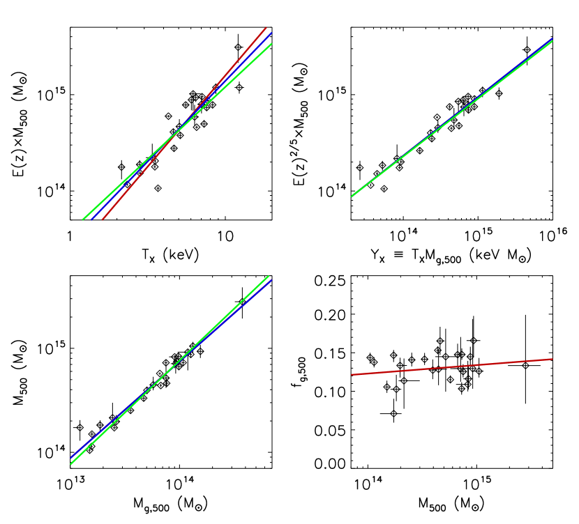
Figure 1: Upper Left: Plot of X-ray spectral temperature, $T_{X}$, and total cluster mass, $M$. Overplotted are the best-fit power-law relations using the BCES orthogonal slope estimator (red), the BCES Y$|$X slope estimator (blue), and a fixed slope of $\alpha=1.5$ (green). Upper Right: Plot of $Y_{X}$ and $M$ with best-fit power-law relations overplotted. Color coding is the same as for the $M-T_{X}$ plot with $\alpha=0.6$. Lower Left: Plot of cluster gas mass, $M_{g}$, and $M$ and best-fit power-law relations overplotted. Color coding is the same as for the $M-T_{X}$ plot with $\alpha=1.0$. Lower Right: Plot of gas mass fraction, $f_{g}$, and $M$. Overplotted is the best-fit relation.

Table 1 and Figure 1 show the best-fit parameters for the $M-T_{X}$ scaling relation. Our best fit ($\log_{10}C=$ 14.64, $\alpha=1.67$) is consistent with the scaling relations found in other datasets (Arnaud et al., 2007; Vikhlinin et al., 2009, $\log_{10}C=$ 14.580 and 14.635, and $\alpha=$ 1.71 and 1.53, respectively). Arnaud et al. (2007) use a different definition of $T_{X}$ which integrates the observed temperature profile over 0.15–0.75 $r_{500}$. Since the average cluster temperature profile falls at large radii (see e.g., Leccardi & Molendi, 2008, A. M. Juett et al. 2009, in prep), this definition will produce higher values of $T_{X}$ and subsequently lower values of the $M-T_{X}$ normalization. We find that $\langle T_{\rm X}(0.15-0.75r_{500})/T_{\rm X}(0.15-1r_{500})\rangle=1.06$, which translates into a reduction of $\log_{10}C$ of 0.04–0.05, enough to explain the discrepancy between our results and Arnaud et al. (2007).

When compared to theoretical calculations (Kravtsov et al., 2006; Nagai et al., 2007a, b; Jeltema et al., 2008), our results are consistent when the hydrostatic mass is considered, but our normalization is lower by $\approx 20$% when compared to scaling results that use the true cluster mass (14.70–14.75). This is a well known result and is likely due to non-thermal pressure support that is not accounted for in the hydrostatic mass estimate (e.g., Nagai et al., 2007a). The biggest difference between our results and previous studies is the difference in scatter around the best-fit scaling relation. We find a scatter of 43% which, due to our systematics limited dataset, can be attributed to the intrinsic scatter of our sample. Other studies, of both observed and theoretical cluster samples, have found significantly lower values for the intrinsic scatter, $\approx 10-25$% (Vikhlinin et al., 2006; Arnaud et al., 2007; Nagai et al., 2007a, b; Jeltema et al., 2008).

3.2 Mass$-$Gas Mass

The gas mass–total mass scaling relationship has been previously characterized in two ways: a powerlaw scaling between $M$ and $M_{g}$, and more recently by a linear scaling of $f_{g}$ and the logarithm of $M$.

Our $M-M_{g}$ results ($\log_{10}C=14.503\pm 0.018$), are in agreement with the normalization found by Arnaud et al. (2007, 14.542$\pm$0.015) considering the small formal errors. But our best-fit slope is steeper (0.93$\pm$0.05 vs 0.80$\pm$0.04). Again we find that theoretical models that use the true cluster mass have higher predicted normalizations but our results are consistent when hydrostatic mass estimates are used (Kravtsov et al., 2006; Nagai et al., 2007a). The slope estimate is consistent with theoretical results for both true and hydrostatic mass estimates. Our 15% scatter is close to the $\approx$10% scatter found in both observational and theoretical work. Interestingly, our results match the combination of normalization, slope, and scatter found in the simulations of Nagai et al. (2007a) when hydrostatic mass is used, however we differ from their Chandra observational results. Our slope is larger (0.93 vs 0.81) while our normalization is lower (14.503 vs 14.59). This discrepancy may be due to differences in the calibration of the instruments that has been previously noted (e.g., Snowden et al., 2008).

We find that the normalization of the $f_{g}-M$ relationship, $0.134\pm 0.005$, is consistent with the value of Vikhlinin et al. (2009, 0.130$\pm$0.007). Our data are consistent with a constant slope over the range of mass considered, while the Vikhlinin et al. (2009) result prefers a reduction in $f_{g}$ for lower mass clusters. The Vikhlinin et al. (2009) result is consistent with gas mass fraction results from groups of galaxies (Sun et al., 2009). Arnaud et al. (2007) suggested that the gas mass fraction may be constant above $2-3\times 10^{14}M_{\odot}$, and then dropping at lower masses. This would explain both our result and the lower gas mass fractions seen in groups of galaxies.

The difference in mean gas mass fraction between the Vikhlinin et al. (2006) work, a subset of the Vikhlinin et al. (2009) sample, and ours is 10–20%. At $r_{500}$, we find a mean $f_{g}=0.1323\pm 0.0019$, compared to 0.110$\pm$0.002 for the Vikhlinin et al. (2006) sample (adjusted to account for differences in cosmology). If we restrict our analysis to clusters with $kT>5$ keV, the difference is $\approx$10%, 0.138$\pm$0.003 for our work compared to 0.123$\pm$0.003 (Vikhlinin et al., 2006).

Our results are also close to those found by Allen et al. (2008). At $r_{2500}$, Allen et al. (2008) found a mean cluster gas mass fraction of 0.113$\pm$0.003 for clusters with $kT>5$ keV and low redshifts ($z<0.15$). For their full sample ($kT>5$ keV but all redshifts) they find a mean $f_{g}=0.1104\pm 0.0016$. Vikhlinin et al. (2006) noted that their mean $f_{g}$ at $r_{2500}$ was significantly less (0.091$\pm$0.002, a $\sim$25% difference) than an earlier (but consistent) Allen et al. sample. We find $f_{g,2500}=0.1057\pm 0.0005$ for clusters with $kT>5$ keV, a 4% difference with the Allen et al. (2008) results and a $\approx$15% difference with the Vikhlinin et al. (2006) work.

3.3 Mass$-Y_{X}$

Kravtsov et al. (2006) suggested that a lower scatter ($<10$%) proxy for cluster mass is the parameter $Y_{X}=T_{X}M_{g}$. Table 1 gives our best-fits for the $M-Y_{X}$ scaling relation. Our best-fit normalization (14.657$\pm$0.018) is consistent with the results of Arnaud et al. (2007, 14.653$\pm$0.015 when renormalized) and Vikhlinin et al. (2009, 14.684$\pm$0.015). When comparing with theoretical results, we find consistency with hydrostatic mass results (14.645) but not true cluster mass (14.712; e.g. Nagai et al., 2007a). The slope of the best-fit $M-Y_{X}$ compares well with both observational and theoretical studies.

The largest difference comes in the measured scatter in the $M-Y_{X}$ relation. We find a scatter of $\approx 22$%, much larger than the $<10$% level expected from simulations. While other observational studies have not found as large a scatter (e.g., Arnaud et al., 2007), we note that ours is the first study to be systematics limited and includes twice the number of objects. Thus we are able to measure the scatter without a significant contribution from the statistical error. In theoretical work, scatter increases to 8–20% when hydrostatic masses are used compared to true masses (Nagai et al., 2007a; Jeltema et al., 2008).

4 Correlation of Deviation with Cluster Properties

Scatter in the mass–X-ray observable relationships is an important contributor to the total error budget in cosmological studies of clusters (see e.g. Vikhlinin et al., 2009). Given our large sample of clusters, we can study what factors are most important in producing scatter in these relationships which can then be used to refine cosmological studies to reduce the scatter.

One possible cause of the observed scatter is the dynamical state of the cluster. Relaxed clusters are expected to better follow the assumptions of hydrostatic equilibrium. Disturbed clusters may have additional pressure and energy inputs due to the merging events and the additional complication of asymmetric geometries (e.g., Nagai et al., 2007b).

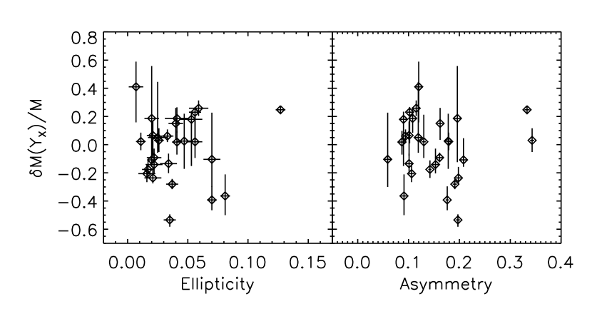
Figure 2: Plot of deviation ($\delta M(Y_{X})/M$) around the best-fit $M-Y_{X}$ scaling relationship versus measures of the cluster dynamical state, ellipticity (left panel) and asymmetry (right panel). No correlation is found.

We looked for correlation between the deviation of the calculated hydrostatic mass, $M_{i}$, from the expected mass given the best-fit scaling relationship, $M(X_{i})$, with measures of the ellipticity and asymmetry in the cluster images (see Figure 2). We identify the deviation as $\delta M(X)/M=[M_{i}-M(X_{i})]/M_{i}$. The ellipticity and asymmetry were calculated following the work of Hashimoto et al. (2007). Relaxed clusters should have low ellipticity and asymmetry values, while disturbed systems will have higher ellipticity and/or asymmetry values. Hashimoto et al. (2007) showed that ellipticity is correlated with the P2/P0 power ratio and that asymmetry is related to the P3/P0 power ratio (see e.g., Buote & Tsai, 1995; Jeltema et al., 2008, for a discussion of power ratios). We find no correlation between the amount of deviation and either ellipticity or asymmetry for any of our scaling laws.

We looked for other cluster properties that might influence the deviation. Vikhlinin et al. (2006) noted that implicit in the calculation of hydrostatic mass, there is a dependence of the normalization of the $M-T_{X}$ relation on the sum of the temperature gradient, $\beta_{t}=(-1/3)\,d\log T/d\log r$, and gas density gradient, $\beta_{eff}=(-1/3)\,d\log\rho/d\log r$ (see their Appendix A). If the spread in values is large enough, this dependence should cause a predictable deviation around the best-fit relationship. We find a strong correlation between $\delta M(X)/M$ and $\beta_{eff}+\beta_{t}$ for all scaling relationships (Figure 3). The Spearman rank correlation coefficients were 0.62, 0.53, and 0.61 for $X=T_{X}$, $M_{g}$, and $Y_{X}$, corresponding to probabilities of 0.9987, 0.9943, and 0.9986, respectively.”

The Vikhlinin et al. (2006) cluster sample has a narrow distribution of $\beta_{eff}+\beta_{t}$ values. Our sample however, shows a large variation in the temperature gradient. For $\beta_{t}$, we find a mean of 0.53 and a standard deviation of 0.50. The range of temperature gradient values is a reflection of the variation of temperature profiles at large radii in our cluster sample (Snowden et al., 2008). The gas density gradient has a narrower distribution with a mean $\beta_{eff}=0.63$ and a standard deviation of 0.10. Our gas density gradient results are in good agreement with those found in the REXCESS study ($\beta_{ne}$ (0.3–0.8 $r_{500}$) = 0.60$\pm$0.10 Croston et al., 2008).

5 Discussion

Our XMM-Newton survey of galaxy clusters (Snowden et al., 2008), provides a large sample and high signal-to-noise data to study the scaling relationships between cluster mass and cluster X-ray temperature, gas mass, gas mass fraction, and the mass proxy $Y_{X}$. Our fits are in good agreement with other observational and theoretical work, with one major caveat. We find a significantly larger scatter around the best-fit relationships than has been previously seen.

The scatter around the best-fit scaling relationships is 2–3 times that found in most other observational and theoretical work. Interestingly, a recent study of the scaling relationship between the Compton y-parameter from SZ studies and cluster masses obtained from gravitational lensing also showed large scatter in the $M_{GL}-T_{X}$ and $M_{GL}-Y$ relationships (41% and 32%, respectively; Marrone et al., 2009), however we note a difference in methodology between their work and ours (Marrone et al. (2009) used a fixed clustercentric radius of 350kpc, while we work in mass scaled units). While other work has suggested that disturbed clusters will show more scatter than relaxed clusters (e.g. Kravtsov et al., 2006), those authors used a visual classification of their simulated clusters, rather than a quantitative determination, making comparison difficult. Within our sample, we find no correlation between measures of the cluster dynamical state (ellipticity and asymmetry) and deviation around the best-fit scaling relationships.

Only one cluster property, the combination $\beta_{eff}+\beta_{t}$, showed a strong correlation with deviation. Since hydrostatic mass estimates, like those used here, depend on this explicitly, the result should be expected (e.g. Vikhlinin et al., 2006). Our data are the first to show this dependence due to the large sample size and range of cluster properties included. There is no reason to suspect that true cluster masses will show such a dependence given the bias (and scatter) in hydrostatic mass determinations found in simulations where the true cluster masses are known (see e.g, Nagai et al., 2007b).

One question we must ask is how reliable are our determinations of the temperature profiles, whose wide range dominates the measurement of $\beta_{eff}+\beta_{t}$. To check the reliability of the background modeling and spectral fitting procedure, Snowden et al. (2008) compared the profile of A1795 with published Chandra, XMM-Newton, and Suzaku temperature profiles and found no significant difference. They also found reproducibility for three clusters with multiple observations. An initial comparison of our average cluster temperature profile is in good agreement with previous results both in overall shape and expected scatter (see A. M. Juett et al. 2009, in prep). The results of Leccardi & Molendi (2008) also suggest that cluster temperature profiles, while generally showing a falling profile at large radii, do show a range of profiles. Followup observations are needed of the most unusual systems to confirm our results.

Assuming our temperature profile range is indicative of the cluster population, we then need to ask how does this result affect cosmological studies using clusters. First, a larger scatter should be taken into consideration when discussing systematic errors in cosmological studies (see e.g. Vikhlinin et al., 2009). However, given other error sources, it is not clear that the mass scaling relationship scatter would be the dominant error contributor.

It may be possible to correct for the scatter from theoretical studies of cluster properties but it is unclear if present models are consistent with our results. Nagai et al. (2007a) find little variation in the temperature profile at $r_{500}$ in their simulations, although these are limited to their relaxed subsample. If a more thorough study of the simulations is not able to reproduce the observed cluster variation, that may point to some missing physics needed to better describe the conditions within clusters.

Another result we would like to highlight is the comparison of our average gas mass fraction with previous results. The differences between our work and others (e.g., Vikhlinin et al., 2006; Allen et al., 2008) range from 5–20%. This is comparable with expected systematic differences between the instruments and analysis methods, but is significantly larger than the statistical errors typically quoted. In our opinion, a study of the expected systematics due to (1) instrumental calibration differences, and (2) data analysis methods must be performed. These issues are beyond the scope of this work, but will be addressed in our future paper (A. M. Juett et al. 2009, in prep).

Figure 3: Plot of deviation around the best-fit mass scaling relations, $\delta M(X)/M$, versus $\beta_{eff}+\beta_{t}$. The results for the scaling relationships for $M-T_{X}$ (top panel), $M-M_{g}$ (middle panel) and $M-Y_{X}$ (bottom panel) are given. All show a correlation between deviation and $\beta_{eff}+\beta_{t}$.

Table 1: Best-Fit Parameters of Powerlaw Fits

Relation	Fit Method	$\log_{10}C/f_{g,0}$	$\alpha$	Scatter
M$-$T	Y$|$X	14.64$\pm$0.03	1.67$\pm$0.16	0.420
	Orth	14.63$\pm$0.03	1.89$\pm$0.20	0.430
	Fix	14.63$\pm$0.03	1.5	0.412
M$-$YX	Y$|$X	14.657$\pm$0.018	0.61$\pm$0.04	0.218
	Orth	14.657$\pm$0.018	0.61$\pm$0.04	0.218
	Fix	14.646$\pm$0.018	0.60	0.212
M$-$Mg	Y$|$X	14.503$\pm$0.018	0.93$\pm$0.05	0.144
	Orth	14.504$\pm$0.017	0.93$\pm$0.05	0.145
	Fix	14.484$\pm$0.013	1.0	0.149
$f_{g}-$M	Y$|$X	0.134$\pm$0.005	0.011$\pm$0.013	0.104
	Orth	0.134$\pm$0.005	0.011$\pm$0.013	0.104

References

- Akritas & Bershady (1996) Akritas, M. G., & Bershady, M. A. 1996, ApJ, 470, 706
- Allen et al. (2008) Allen, S. W., Rapetti, D. A., Schmidt, R. W., Ebeling, H., Morris, R. G., & Fabian, A. C. 2008, MNRAS, 383, 879
- Arnaud et al. (2007) Arnaud, M., Pointecouteau, E., & Pratt, G. W. 2007, A&A, 474, L37
- Buote & Tsai (1995) Buote, D. A., & Tsai, J. C. 1995, ApJ, 452, 522
- Croston et al. (2008) Croston, J. H., et al. 2008, A&A, 487, 431
- Hashimoto et al. (2007) Hashimoto, Y., Böhringer, H., Henry, J. P., Hasinger, G., & Szokoly, G. 2007, A&A, 467, 485
- Jeltema et al. (2008) Jeltema, T. E., Hallman, E. J., Burns, J. O., & Motl, P. M. 2008, ApJ, 681, 167
- Kravtsov et al. (2006) Kravtsov, A. V., Vikhlinin, A., & Nagai, D. 2006, ApJ, 650, 128
- Leccardi & Molendi (2008) Leccardi, A., & Molendi, S. 2008, A&A, 486, 359
- Marrone et al. (2009) Marrone, D. P., et al. 2009, ApJ, 701, L114
- Nagai et al. (2007a) Nagai, D., Kravtsov, A. V., & Vikhlinin, A. 2007a, ApJ, 668, 1
- Nagai et al. (2007b) Nagai, D., Vikhlinin, A., & Kravtsov, A. V. 2007b, ApJ, 655, 98
- Pratt et al. (2009) Pratt, G. W., Croston, J. H., Arnaud, M., & Böhringer, H. 2009, A&A, 498, 361
- Rapetti et al. (2008) Rapetti, D., Allen, S. W., & Mantz, A. 2008, MNRAS, 388, 1265
- Snowden et al. (2008) Snowden, S. L., Mushotzky, R. F., Kuntz, K. D., & Davis, D. S. 2008, A&A, 478, 615
- Sun et al. (2009) Sun, M., Voit, G. M., Donahue, M., Jones, C., Forman, W., & Vikhlinin, A. 2009, ApJ, 693, 1142
- Vikhlinin (2006) Vikhlinin, A. 2006, ApJ, 640, 710
- Vikhlinin et al. (2009) Vikhlinin, A., et al. 2009, ApJ, 692, 1033
- Vikhlinin et al. (2006) Vikhlinin, A., Kravtsov, A., Forman, W., Jones, C., Markevitch, M., Murray, S. S., & Van Speybroeck, L. 2006, ApJ, 640, 691
- Voit (2005) Voit, G. M. 2005, Reviews of Modern Physics, 77, 207