Normalization procedure for relaxation studies in NMR quantum information processing

Abstract

NMR quantum information processing studies rely on the reconstruction of the density matrix representing the so-called pseudo-pure states (PPS). An initially pure part of a PPS state undergoes unitary and non-unitary (relaxation) transformations during a computation process, causing a “loss of purity” until the equilibrium is reached. Besides, upon relaxation, the nuclear polarization varies in time, a fact which must be taken into account when comparing density matrices at different instants. Attempting to use time-fixed normalization procedures when relaxation is present, leads to various anomalies on matrices populations. On this paper we propose a method which takes into account the time-dependence of the normalization factor. From a generic form for the deviation density matrix an expression for the relaxing initial pure state is deduced. The method is exemplified with an experiment of relaxation of the concurrence of a pseudo-entangled state, which exhibits the phenomenon of sudden death, and the relaxation of the Wigner function of a pseudo-cat state.

1 Introduction

The dynamics of open quantum systems has been used for a long time to study physical ideas behind quantum measurements and decoherence pazzurek01 . Special attention has been devoted to those aspects of open quantum evolution which are relevant to understand the transition from quantum to classical regimes. Recently, the need for the maintenance of quantum state coherence, for quantum computation and communication tasks nielsen2000 , has increased the interest in dynamical properties of open quantum systems. In general, relaxation occurs as a result of the coupling of the system with the environment, which leads to loss of coherence, being characterized mainly by energy relaxation and phase randomization rates vandersypen04 . Energy dissipation carries away energy quanta on the scale of the Larmor frequency by enabling the spins to flip amongst their energy levels so as to establish the equilibrium populations differences. Phase randomization destroys the coherences due to inhomogeneities and fluctuations in the environment. Furthermore, for nuclear spin systems with $I>1/2$, additional quadrupolar interactions also leads to relaxation when modulated by the environment. Recently, theoretical as well as experimental studies about the nature of the spin-environment coupling have been reported zurek82 ; teklemariam03 ; nagele08 .

On the other hand, Nuclear Magnetic Resonance (NMR) has been successfully used as an experimental method for many Quantum Information Processing (QIP) implementations ivan2007 . Generally, the NMR density matrix is written in the form:

$$\rho_{\epsilon}=(1-\epsilon)\rho_{I}+\epsilon\rho_{1}$$

where $\rho_{I}$ is the (normalized) identity matrix, and $\rho_{1}$ is an arbitrary density matrix braunstein99 . $\epsilon$ is a parameter varying between 0 and 1, which is basically the ratio between the magnetic and thermal energies. For liquid samples at room temperature, $\epsilon\approx 10^{-5}$, what makes $\rho_{\epsilon}$ a highly mixed state, close to the maximum entropy one.

In most NMR QIP implementations, the experiment is carried out in an ensemble of spins in such a highly mixed state. Upon a set of unitary and non-unitary operations, the density matrix $\rho_{1}$ can be transformed into a pure state, $|\psi\rangle\langle\psi|$. In this situation, $\rho_{\epsilon}$ is called a pseudo-pure state cory97 .

Pseudo-pure states allow exploring ensemble quantum computing using NMR technique because, upon unitary transformations, which form the basis of quantum logic gates and algorithms, only the pure deviation matrix evolves. The identification of the pure part of the pseudo-pure density matrix can be made from quantum state tomography technique (QST).

However, PPS states are non-equilibrium states, and they relax back to a Boltzmann distribution in a NMR characteristic time T₁, the longitudinal (spin-lattice) relaxation time. Besides, NMR coherences vanish in a time T₂, the transverse relaxation time. Regarding relaxation studies of pseudo-pure states in the context of NMR quantum information processing, one can point out the studies reported on references sarthour2003 ; ghosh2005 ; boulant03 ; auccaise2008 . In those studies, relaxation behavior of various pseudo-pure states have been investigated in different NMR systems. In reference sarthour2003 it was found that spin-lattice relaxation followed multi-exponential model that included mixed magnetic dipolar and electric quadrupolar interactions. In Ref. ghosh2005 it was found that whereas cross-correlations accelerate the relaxation of certain pseudo-pure states, they delay that of others. On the other hand, a robust method for quantum process tomography provided a set of Lindblad operators that optimally fit the density matrices measured at a sequence of time points boulant03 .

In spite of the various studies cited above, to the best of our knowledge, there is no report showing how the initial pure part evolves under relaxation processes. Yet, it is just this part of the density matrix that matters for NMR QIP analysis. The reason is that there is no simple normalization procedure to keep the deviation part of $\rho_{\epsilon}$ a true density matrix along the relaxation. Therefore, it would be desirable to have a way to follow the evolution of an initial PPS state which undergoes a relaxation process $|\psi\rangle\langle\psi|\rightarrow\rho_{1}$, yet keeping the properties of a density matrix for the deviation, all the way through. This would allow the study of other important quantum information observables under relaxation. In this paper we propose such a method. To illustrate it, we analyze experimental data for the concurrence of initially pseudo-entangled states and the discrete Wigner functions of a relaxing quadrupolar spin 3/2.

The paper is organized as follows: In Sec.2 we show that there is no trivial normalization procedure for the deviation density matrix, and that fixed normalization schemes produces invalid density matrices. In Sec.3 we develop a normalization procedure that produces valid relaxing density matrices. Finally, in Sec.4 we present some application examples of the method.

2 Time-Independent Normalizing procedure for the deviation density matrix

The density matrix formalism is an appropriate description for both, pure and mixed quantum states nielsen2000 . Here, we consider a general density matrix for a spin ensemble with the form:

$$\rho=\rho_{I}+\sigma$$ (1)

where $\rho_{I}=\mathbf{1}/N$ represents a maximally mixed state and $\sigma$ is called deviation density matrix suter2009 . This type of density matrix appears, for instance, from spin ensemble coupled to a heat reservoir at a fixed temperature and whose thermal energy is much bigger than the magnetic energy of nuclear moments in the ensemble. This is called the high-temperature approximation.

For some systems with zero trace observables, such as the case of NMR, only $\sigma$ can be experimentally observed. This means that quantum information quantities, such as the concurrence, entropy or Wigner functions, among others, cannot be directly obtained from experimental data; for that a true density matrix is necessary.

We consider now a quantum process described by a trace preserving quantum operation $\mathcal{S}$. Applying such operator to the density matrix Eq.(1) yields

$$\mathcal{S}\left(\rho\right) = \mathcal{S}\left(\rho_{I}\right)+\mathcal{S}\left(\sigma\right)$$ (2)

$$= \rho_{I}+\left[\mathcal{S}\left(\rho_{I}\right)-\rho_{I}+\mathcal{S}\left(\sigma\right)\right],$$ (3)

which has the same form as (1), if we make the identification:

$$\sigma\overset{\mathcal{S}}{\longrightarrow}\left[\mathcal{S}\left(\rho_{I}\right)-\rho_{I}\right]+\mathcal{S}\left(\sigma\right),$$ (4)

This shows that the process $\mathcal{S}$ is not generally linear in $\sigma$. The linearity of $\mathcal{S}$ with respect to $\sigma$ is only obtained if $\mathcal{S}$ is a unital process ($\mathcal{S}(\mathbf{1})=\mathbf{1}$), for instance, unitary transformations, which is not the case for most relaxation phenomena garcia-mata2005 . Trace-preserving unital processes are the quantum analogs of the classical doubly stochastic processes, which can only increase the von-Neumann entropy of a state (defined to be $-$Tr$\left\{\rho\text{log}\rho\right\}$). Otherwise, non-unital processes provide the only means to reduce entropy and prepare initial states leung . Usually in quantum algorithms applications, the identity term of the Eq.(1) can be neglected because it is invariant under unital processes.

In order to illustrate a relaxation process $\mathcal{S}$ acting on the density matrix, the deviation density matrix obtained from Redfield theory for a purely quadrupolar relaxation of an ensemble of spin $I=3/2$ will be considered (the deviation density matrix elements are on Appendix A). We consider as initial state a pseudo-pure state

$$\rho_{\epsilon}=\left(1-\epsilon\right)\rho_{I}+\epsilon|\psi\rangle\langle\psi|,$$ (5)

where $|\psi\rangle$ is a pure state. It could be, for instance, the pure state $|11\rangle$. From (5) we have:

$$|11\rangle\langle 11| = \frac{1}{\epsilon}\left[\rho_{\epsilon}-\left(1-\epsilon\right)\rho_{I}\right]$$ (6)

$$= \frac{1}{\epsilon}\sigma+\rho_{I}.$$ (7)

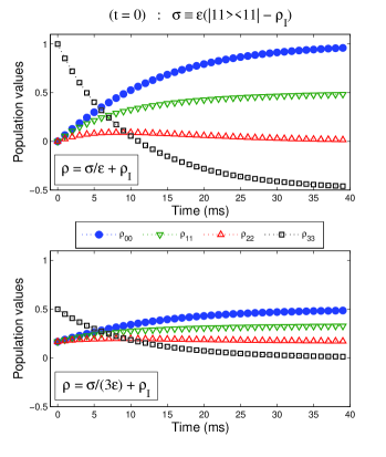
Figure 1: Calculated population values of the initial computational basis state $|11\rangle$ evolving under pure quadrupolar relaxation. The top and bottom plots represent two different types of time-fixed normalization to deviation density matrix, from which we obtain the pure part of the pseudo-pure state (see Appendix A for details). On the top scheme the matrix population become negative after 10 ms. On the bottom one populations are positive, but their initial values are incorrect.

Hence, normalizing the deviation density matrix by $\epsilon$ and adding to $\rho_{I}$ the pure state can be obtained. But, since $\sigma$ changes with evolving time due to quadrupolar relaxation process, the loss of purity will make the pure state $|11\rangle$ to change to a mixed state. In Fig. 1 (top) is shown the relaxation of the population (diagonal matrix elements) of the $|11\rangle$ state. This was obtained considering fixed normalization, like Eq.(7) for $\sigma$ varying in time. Since populations assume negative values at times above $10$ ms, one no longer has a valid density matrix. Therefore, maintaining the normalization of the Eq.(7), leads to matrices exhibiting negative populations at some instants of time. On another hand, if we try adjusting the final population values, the equilibrium state $\rho_{eq}$, we can use the following normalization

$$\rho_{eq}=\frac{1}{\epsilon^{\prime}}\sigma+\rho_{I}$$ (8)

such that the $\rho_{eq}$ has trace equal $1$ and non-negative populations. In this case (electric quadrupole relaxation to $3/2$ nuclear spin) $\epsilon^{\prime}=3\epsilon$. It can be seen in Fig. 1 (bottom) that they have non-negative values for the whole interval of time, but at $t=0$ we have incorrect populations values for the pseudo-pure state. Thus we also discard this method of normalization.

From these two different ways to normalize initial and final deviation matrices, we can conclude that the normalization must be time-dependent.

3 Time-Dependent Normalization Method

First we will consider initial and final conditions for $\rho(t)$. Re-writing (5) in a slightly different way, we have the pseudo-pure state,

$$\rho(t=0) = \rho_{I}+\epsilon\left(|\psi\rangle\langle\psi|-\rho_{I}\right).$$ (9)

In words, the pseudo-pure state is composed by a maximum statistical mixture, $\rho_{I}$, and a pure contribution $|\psi\rangle$.

Under relaxation, the system reaches the equilibrium state. For this state one can consider the Zeeman interaction as the most important one. In the high-temperature limit:

$$\rho(t\rightarrow\infty) = \frac{e^{\beta\hbar\omega I_{z}}}{Tr\left(e^{\beta\hbar\omega I_{z}}\right)}\approx\rho_{I}+\frac{\hbar\beta\omega}{N}I_{z}$$ (10)

$$= \rho_{I}+2I\epsilon\left(\rho_{z}-\rho_{I}\right),$$

where $I$ is the angular momentum of the nuclear spin and $\epsilon=\hbar\beta\omega/2$, and $\rho_{z}\equiv(1/NI)I_{z}+\rho_{I}$.

From this, we can write for the respective initial and final (equilibrium) deviation matrices: $\sigma_{0}=\epsilon\left(|\psi\rangle\langle\psi|-\rho_{I}\right)$ and $\sigma_{\infty}=2I\epsilon\left(\rho_{z}-\rho_{I}\right)$. The initial deviation matrix has “polarization” $\epsilon$, whereas the equilibrium has “polarization” $2I\epsilon$. The relaxation phenomenon connects these two matrices in time. Therefore, we can write a general form for a deviation density matrix:

$$\sigma=\alpha\left(\rho_{\alpha}-\rho_{I}\right),$$ (11)

where $\alpha$ is the polarization and $\rho_{\alpha}$ the respective density matrix. From $\alpha$ and $\rho_{I}$, $\rho_{\alpha}$ can be determined for any deviation density matrix $\sigma$.

Adding $\sigma_{0}$ to both sides of the Eq. (11) and isolating $\rho_{\alpha}$, we have:

$$\rho_{\alpha}=\frac{\epsilon}{\alpha}|\psi\rangle\langle\psi|+\frac{1}{\alpha}\left[\sigma-\sigma_{0}\right]+\left(1-\frac{\epsilon}{\alpha}\right)\rho_{I}.$$ (12)

This is the final expression for the density matrix for a given $\alpha$ and $\sigma$. For example, at $t=0$, $\alpha=\epsilon$ and $\sigma=\sigma_{0}$, and we are left with a pure state. Upon relaxation the other terms come into action. Notice that the first and last terms on the right side can be interpreted as a depolarization channel nielsen2000 , whereas the middle term depends on the relaxation model, for instance, the Redfield theory. $\alpha$ is a time-adjustable parameter, which varies in the interval $(0,2I\epsilon]$. It is worth mentioning that there is a possible connection between $\alpha$ and the effective number of nuclei per state cory97 .

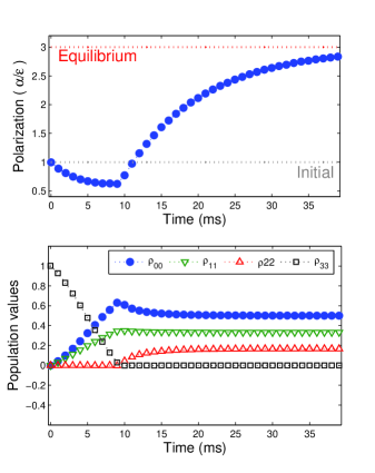
Figure 2: Time evolution of the polarization and respective normalized populations for spin $3/2$ nuclei in the initial state $|11\rangle\langle 11|$.

Eq.(12) can be used to obtain the properly normalized density matrix $\rho_{\alpha}$, at any instant of time, from the measured deviation density matrices. A numerical example is shown on Fig. 2, for the same parameters used to calculate the data on Fig. 1. At any instant of time the populations add $1$ and never become negative. Next we will analyze experimental results for pseudo-entangled states and Wigner functions.

4 Experimental results

²³Na NMR experiments were performed using a magnetic field oriented lyotropic liquid-crystal system (Sodium Dodecyl Sulfate, SDS), using a 9.4 T - VARIAN INOVA spectrometer. The sample composition was 21.3$\%$ of SDS, 3.6$\%$ of decanol, and 75.1$\%$ of deuterium oxide. The quadrupolar coupling was found to be (16700 $\pm$ 70) Hz at 24 ^∘C. In the experiments that characterized the relaxation of all elements of the density matrix, an initial pseudo-pure state was prepared using the SMP technique fortunato2002 . In this case, all the deviation density matrix elements were measured using the QST method via coherence selection teles2007 . The basic experimental scheme consisted of: i) a state preparation period performed with SMP; ii) a variable evolution period $\tau$ where relaxation takes place; and iii) a hard RF pulse with the correct phase cycling and duration to execute QST via coherence selection, as described in detail in Ref. auccaise2008 .

4.1 Computational basis states

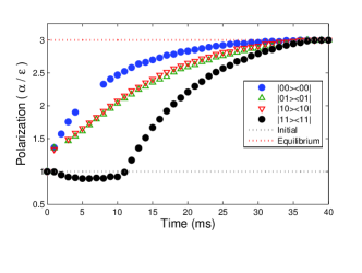
Figure 3: Polarization for computational basis states encoded in the spin $3/2$ nuclei. Also the initial and equilibrium limits to polarization are shown. Notice that initial polarizations are $\epsilon$, whereas final ones are $2I\epsilon$. Experimental data taken from previous experiments auccaise2008 .

In Fig. 3 we show some $\alpha$-polarization curves for different initial states, namely the computational basis states $|00\rangle$, $|01\rangle$, $|10\rangle$ and $|11\rangle$, obtained from experimental relaxation results auccaise2008 .

The density matrix for a computational basis state is diagonal and the “polarization” for each of these states is different. This happens because the relaxation acts differently on each diagonal elements of the density matrix. Since each state population relax at a different rate sarthour2003 , the normalization will also be different.

4.2 Pseudo-entangled state

Entanglement is a quantum correlation that reveals nonlocal properties of a given system. In order to compute such correlation or, in other words, to measure the degree of entanglement within the system, it is possible to use the concept of concurrence wootters98 . For a given density matrix $\rho$, the concurrence can be written as:

$$\mathcal{C}(\rho)=\mbox{max}\left\{0,\sqrt{\lambda_{1}}-\sqrt{\lambda_{2}}-\sqrt{\lambda_{3}}-\sqrt{\lambda_{4}}\right\},$$ (13)

where the $\lambda_{i}$s are the eigenvalues, in decreasing order, of the matrix $R\equiv\rho(\sigma_{y}\otimes\sigma_{y})\rho^{*}(\sigma_{y}\otimes\sigma_{y})$. It is important to note that for density matrices like

$$\rho=\left[\begin{array}[]{cccc}a&0&0&w\\ 0&b&z&0\\ 0&z^{*}&c&0\\ w^{*}&0&0&d\end{array}\right],$$ (14)

named $X-$state, the concurrence has a analytical solution given by:

$$\mathcal{C}(\rho)=2\,\mbox{max}\left\{0,\mathcal{C}^{I};\mathcal{C}^{II}\right\},$$ (15)

where $\mathcal{C}^{I}=|z|-\sqrt{a\,d}$ e $\mathcal{C}^{II}=|w|-\sqrt{b\,c}$ fubini06 ; yu07 .

For a NMR system, described by Eq.(5), it was shown that even being $|\psi\rangle$ a pure entangled state, i.e., a Bell basis state, the total density matrix is always separable braunstein99 . It happens because the polarization is very small ($\epsilon\approx 10^{-5}$, as said before), meaning that the density matrix is highly mixed. However, NMR is still capable to reproduce the correct dynamics of such pseudo-entangled states, since they behave like pure entangled ones linden01 .

Many works have been done about the dynamics of entanglement yu2002 ; simon2002 ; dur2004 ; yu09 . It was always expected that the dynamics of the concurrence would give an asymptotic decay of the degree of entanglement, since it is the typical behavior of the decoherence processes. However, for some quantum states it was reported a curious phenomenon, named sudden death of entanglement, where the degree of entanglement vanishes at a finite time yu09 . It has been recently measured in optical salles08 and atomic laurat07 systems.

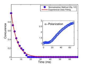
Figure 4: Concurence decay of pseudo-entangled initial state $2^{-1/2}\left(|00\rangle+|11\rangle\right)$. The data were obtained from experimental deviation density matrices of the relaxation of ²³Na nuclei, normalized by the procedure developed in the section 3. The solid line is the exponential fitting, included for comparison. The $\alpha$-polarization curve utilized to normalize the relaxing pseudo-cat state are the inside plot.

Fig. 4 shows a NMR experiment of the sudden death of entanglement of the pseudo-entangled state $|\psi^{+}\rangle=(|00\rangle+|11\rangle)/\sqrt{2}$, where its concurrence for such state is given by $\mathcal{C}^{I}$ term, using the normalization procedure described in Sec. III on the relaxation of ²³Na. The continuous line is an exponential fit, included for comparison (asymptotic decay). We can clearly see that the concurrence vanishes at a finite time just below 20 ms, which is the same order of the transverse relaxation time of the sample.

4.3 Discrete Wigner Function

Another usual description to quantum states is the Wigner function formalism, which consists on the representation of a quantum state in the phase-space. Wigner functions can be obtained from the so called “phase space point operators” wootters87 . They can be defined as the following expectation value:

$$W(q,p)=\mbox{Tr}\left[\hat{\rho}\hat{A}(q,p)\right],$$ (16)

where the $\hat{A}(q,p)$ are the (Hermitian) phase space point operators and $\hat{\rho}$ is the density operator. Because we are working with discrete spin systems, it is more adequate the use of discrete Wigner functions miquel02 . Such a description is made upon periodic boundary conditions for both, position and momentum (geometry of a torus on the phase-space). In what follows, we will use the density operators (Eq.12) relative to the relaxing pseudo-entangled state $2^{-1/2}\left(|00\rangle+|11\rangle\right)$. The corresponding phase-space point operators in matrix representation are shown on Appendix B.

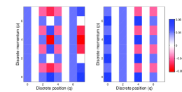
(a) Theoretical: initial and equilibrium

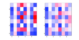
(b) Experimental: $3$ ms and $12$ ms

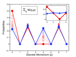
(c) Momentum distribution

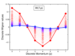
(d) The oscillating term of the Wigner function

Figure 5: The decoherence of the pseudo-entangled state observed from quadrupolar relaxation. In (a) and (b) are theoretical and experimental discrete Wigner functions, where the blue(red) squares represent the positive(negative) values and white squares are null values. Horizontal(vertical) axis is the position(momentum) coordinates. The temporal evolution are shown in (c) for the discrete momentum distribution and in (d) for the oscillating term $W(7,p)$. Red(Blue) dots are the initial(final) values and the inside plot are the initial(red) and final(blue) momentum distribution for only even momentum.

The decoherence of superimposed localized wave packets is a well-known subject in the literature zurek2002 ; schlosshauer07 . The Wigner function for the cat-state exhibits two well separated positive peaks and a non-classical interference pattern between them, which oscillates between positive and negative values. Such oscillations vanish due to the coupling of the system to the environment, leading to a quantum-to-classical transition. Fig. 5 shows NMR results for the Wigner function of the cat-state $2^{-1/2}\left(|00\rangle+|11\rangle\right)$ undergoing relaxation towards equilibrium. The duration of the experiment is about 70 ms. Fig. 5(a) shows the discrete phase-space representation of this state (left), as well as the equilibrium state (right). Notice that $W(0,p)$ and $W(6,p)$ are positive, whereas $W(7,p)$ is an oscillating stripe between them. The oscillation of $W(2,p)$ and $W(4,p)$ are due to the use of periodic boundary conditions and the application of the discrete Fourier transform to obtain the momentum miquel02 . Such “images” are important for the calculation of the marginal momentum from $\sum_{q=0}^{2N-1}W(q,p)$ to guarantee it as a regular probability distribution. Fig. 5(b) shows the same plot as (a) for 3 and 12 ms, but now normalized according to the method described in Sec. III. We can clearly see the changes in the Wigner function caused by quadrupolar relaxation, in particular the interference pattern.

Time-evolution of the momenta distribution can be seen on the bottom of Fig. 5(c). The initial distribution are the red bullets, ($\bullet$), whereas the blue one ($\bullet$) are the final values. Intermediate values are the open dots ($\circ$). From the plot we can see that momenta evolves from a localized $p=0$ value, to become homogeneous (better seen in the inset, only for even values of momentum). This is an indication that there is no localization henry2006 , in the sense that it occurs in classically chaotic quantum maps. Finally, Fig. 5(d) exhibits the time-evolution of the interference term, $W(7,p)$. One can clearly see the decoherence by comparing the initially red points ($\bullet$) to the final blue ones ($\bullet$).

5 Conclusion

In this work a method for the normalization of the initially pure part of a pseudo-pure NMR state undergoing relaxation was presented. The method allows following directly the pure part of $\rho$, whereas keeping it a true density matrix, which is interesting for the the purpose of NMR quantum information processing experiments. We exemplified the method studying the relaxation of initially pseudo-entangled states in which the phenomenon of sudden-death is observed, and the decoherence of Wigner functions in phase-space. The method is particularly useful for relaxation studies in the context of NMR quantum information processing, an area which still lacks experimental data.

Appendix A Redfield theory of pure quadrupolar relaxation spin $3/2$

The spin $3/2$ system dynamics under the presence of relaxation processes can be described using the Redfield formalism for the deviation density matrix abragam . The Hamiltonian that describes a $I>1/2$ spin system in the laboratory frame, considering Zeeman and first order quadrupolar interaction can be expressed as

$$\mathcal{H}=-\hbar\omega_{L}I_{z}+\frac{\hbar\omega_{Q}}{6}\left(3I_{z}^{2}-I(I+1)\right).$$ (17)

The first term describes the Zeeman interaction (with Larmor frequency of $\omega_{L}$) and the second the static first order quadrupolar interaction (with quadrupolar frequency of $\omega_{Q}$). Hence, for nuclear spin $I=3/2$ the eigenvectors of the Zeeman plus quadrupolar terms are $|3/2\rangle$, $|1/2\rangle$, $|-1/2\rangle$ and $|-3/2\rangle$, which can be labeled as $|00\rangle$, $|01\rangle$, $|10\rangle$ and $|11\rangle$, corresponding to a two-qubit system. Here to simplify the expressions of the solutions ($\sigma$) of the Redfield theory found in auccaise2008 we utilize $\Delta=\sigma-\sigma_{\infty}$. The characterization of the relaxation process is performed by means of reduced spectral densities, which contain the information about the local field fluctuations johan91 ; auccaise2008 . Furthermore, when $|\omega_{Q}|\ll|\omega_{L}|$, the relaxation can be described by three reduced densities at the Larmor frequency. Below we show $\Delta$ matrix elements in time function,

$$\Delta_{12}\left(t\right)=\Delta_{12}e^{-t/\tau_{12}},$$ (18)

$$\Delta_{03}\left(t\right)=\Delta_{03}e^{-t/\tau_{12}},$$ (19)

$$\Delta_{01}\left(t\right)=\left[\frac{\left(1+e^{-t/\tau_{2}}\right)}{2}\Delta_{01}+\frac{\left(1-e^{-t/\tau_{2}}\right)}{2}\Delta_{23}\right]e^{-t/\tau_{01}},$$ (20)

$$\Delta_{23}\left(t\right)=\left[\frac{\left(1-e^{-t/\tau_{2}}\right)}{2}\Delta_{01}+\frac{\left(1+e^{-t/\tau_{2}}\right)}{2}\Delta_{23}\right]e^{-t/\tau_{01}},$$ (21)

$$\Delta_{02}\left(t\right)=\left[\frac{\left(1+e^{-t/\tau_{1}}\right)}{2}\Delta_{02}+\frac{\left(1-e^{-t/\tau_{1}}\right)}{2}\Delta_{13}\right]e^{-t/\tau_{02}},$$ (22)

$$\Delta_{13}\left(t\right)=\left[\frac{\left(1-e^{-t/\tau_{1}}\right)}{2}\Delta_{02}+\frac{\left(1+e^{-t/\tau_{1}}\right)}{2}\Delta_{13}\right]e^{-t/\tau_{02}},$$ (23)

$$\Delta_{00}\left(t\right)= \left[\frac{\left(e^{-t/\tau_{2}}+e^{-t/\tau_{1}}\right)}{2}\Delta_{00}+\frac{\left(-e^{-2t/\tau_{12}}+e^{-t/\tau_{2}}\right)}{2}\Delta_{11}+\right.$$ (24)

$$+\left.\frac{\left(-e^{-2t/\tau_{12}}+e^{-t/\tau_{1}}\right)}{2}\Delta_{22}\right],$$

$$\Delta_{11}\left(t\right)= \left[\frac{\left(e^{-t/\tau_{2}}-e^{-t/\tau_{1}}\right)}{2}\Delta_{00}+\frac{\left(e^{-2t/\tau_{12}}+e^{-t/\tau_{2}}\right)}{2}\Delta_{11}+\right.$$ (25)

$$+\left.\frac{\left(e^{-2t/\tau_{12}}-e^{-t/\tau_{1}}\right)}{2}\Delta_{22}\right],$$

$$\Delta_{22}\left(t\right)= \left[\frac{\left(-e^{-t/\tau_{2}}+e^{-t/\tau_{1}}\right)}{2}\Delta_{00}+\frac{\left(e^{-2t/\tau_{12}}-e^{-t/\tau_{2}}\right)}{2}\Delta_{11}+\right.$$ (26)

$$+\left.\frac{\left(e^{-2t/\tau_{12}}+e^{-t/\tau_{1}}\right)}{2}\Delta_{22}\right],$$

$$\Delta_{33}\left(t\right)= -\left[\frac{\left(e^{-t/\tau_{2}}+e^{-t/\tau_{1}}\right)}{2}\Delta_{00}+\frac{\left(e^{-2t/\tau_{12}}+e^{-t/\tau_{2}}\right)}{2}\Delta_{11}+\right.$$ (27)

$$+\left.\frac{\left(e^{-2t/\tau_{12}}+e^{-t/\tau_{1}}\right)}{2}\Delta_{22}\right],$$

where the elements $\Delta_{kl}$ from right side are initial values of them ($\Delta=\sigma_{0}-\sigma_{\infty}$). In addition, the characteristic times $\tau$ are defined as function of the inverse averaged reduced spectral densities auccaise2008 . The characteristic times were determined from previous work as: $\tau_{01}=4.6$, $\tau_{02}=4.7$, $\tau_{12}=11.1$, $\tau_{12}=20.8$ and $\tau_{2}=23.8$ in miliseconds.

Appendix B Matrix representation to phase space point operators

The phase space point operators are a set of Hermitian operators, which gives all marginal distributions obtained from the Wigner function miquel02 . They are defined on a phase space grid of $2N\times 2N$ points

$$\hat{A}(q,p)=\frac{1}{2N}\hat{U}^{q}\hat{R}\hat{V}^{-p}\mbox{exp}(i\pi qp/N),$$ (28)

where $\hat{U}$ is a cyclic shift operator in the computational basis ($\hat{U}|q\rangle=|q+1\rangle$), $\hat{V}$ is a cyclic shift operator in the basis related to the computational basis via the discrete Fourier transform and $\hat{R}$ is the reflection operator ($\hat{R}|q\rangle=|N-q\rangle$). The phase space point operator form a complete orthonormal basis of the space of operators and

$$\hat{A}(q+\xi_{q}N,p+\xi_{p}N)=\hat{A}(q,p)(-1)^{\xi_{p}q+\xi_{q}p+\xi_{q}\xi_{p}N},$$ (29)

for $\xi_{q},\xi_{q}=0,1$. For this reason, it is clear that the $N^{2}$ phase space point operators corresponding to the first $N\times N$ subgrid of the determine the rest.

NMR $3/2$ spin system have four eigenstates (computational basis, $|3/2\rangle$, $|1/2\rangle$, $|-1/2\rangle$ and $|-3/2\rangle$). Thus, the Hilbert space dimension is $N=4$. The operators $\hat{A}(q,p)$ in matrix representation are shown below:

$$A(0,p)=\frac{1}{8}\left(\begin{array}[]{cccc}1&0&0&0\\ 0&0&0&i^{p}\\ 0&0&(-1)^{p}&0\\ 0&(-i)^{p}&0&0\end{array}\right),$$ (34)

$$A(1,p)=\frac{e^{i\pi p/N}}{8}\left(\begin{array}[]{cccc}0&1&0&0\\ i^{p}&0&0&0\\ 0&0&0&(-1)^{p}\\ 0&0&(-i)^{p}&0\end{array}\right),$$ (39)

$$A(2,p)=\frac{e^{i2\pi p/N}}{8}\left(\begin{array}[]{cccc}0&0&1&0\\ 0&i^{p}&0&0\\ (-1)^{p}&0&0&0\\ 0&0&0&(-i)^{p}\end{array}\right),$$ (44)

$$A(3,p)=\frac{e^{i3\pi p/N}}{8}\left(\begin{array}[]{cccc}0&0&0&1\\ 0&0&i^{p}&0\\ 0&(-1)^{p}&0&0\\ (-i)^{p}&0&0&0\end{array}\right).$$ (49)

The projection of the density matrix $\rho$ in these matrices (Eq.16) yields a grid with only real values which represents the density matrix in discrete phase space.

References

- (1) Paz, J.P., Zurek, W.H.: Environment-induced and the transition from quantum to classical. In: Kaiser, R., Westbrook, C., Davids, F. (eds.) Coherent Matter Waves, Proceedings of the Les Houches Session LXXII, pp. 533-614. Springer Verlag, Berlin (2001)
- (2) Nielsen, M.A., Chuang, I.L.: Quantum Computation and Quantum Information. Cambridge University Press, Cambridge (2000)
- (3) Vandersypen, L.M.K, Chuang, I.L.: NMR techniques for quantum control and computation. Rev. Mod. Phys. 76, 1037-1069 (2004)
- (4) Zurek, W.H.: Environment-induced superselection rules. Phys. Rev. D 26, 1862-1880 (1982)
- (5) Teklemariam, G., Fortunato, E.M., López, C.C., Emerson, J., Paz, J.P., Havel, T.F., and Cory, D.G.: Method for modeling decoherence on a quantum-information processor. Phys. Rev. A 67, 062316 (2003)
- (6) Nägele, P., Campagnano, G., Weiss, U.: Dynamics of dissipative coupled spins: decoherence, relaxation and effects of a spin-boson bath. New J. Phys. 10, 115010 (2008)
- (7) Oliveira, I.S., Bonagamba, T.J., Sarthour, R.S., Freitas, J.C.C., deAzevedo, E.R.: NMR quantum information processing. Elsevier, Amsterdam (2007)
- (8) Braunstein, S.L., Caves, C.M., Jozsa, R., Linden, N., Popescu, S., Schack, R.: Separability of Very Noisy Mixed States and Implications for NMR Quantum Computing. Phys. Rev. Lett. 83, 1054 (1999)
- (9) Suter, D., Mahesh, T.S.: Spins as qubits: Quantum information processing by nuclear magnetic resonance. J. Chem. Phys. 128, 052206 (2008)
- (10) Cory, D.G., Fahmy, A.F., Havel, T.F.: Ensemble quantum computing by NMR spectroscopy. Proc. Natl. Acad. Sci. USA, 94, pp. 1634-1639 (1997)
- (11) Sarthour, R.S., deAzevedo, E.R., Bonk, F.A., Vidoto, E.L.G., Bonagamba, T.J., Guimarães, A.P., Freitas, J.C.C., Oliveira, I.S.: Relaxation of coherent states in a two-qubit NMR quadrupole system. Phys. Rev. A 68, 022311 (2003)
- (12) Ghosh, A., Kumar, A.: Relaxation of pseudo pure states: the role of cross-correlations. J. Magn. Res. 173, 125-133 (2005)
- (13) Boulant, N., Havel, T.F., Pravia, M.A., Cory, D.G.: Robust method for estimating the Lindblad operators of a dissipative quantum process from measurements of the density operator at multiple time points. Phys. Rev. A 67, 042322 (2003)
- (14) García-Mata, I., Saraceno, M., Spina, M.E., Carlo, G.: Phase-space contraction and quantum operations. Phys. Rev. A 72, 062315 (2005)
- (15) Leung, D., PhD. theses, Stanford University (2002)
- (16) Fortunato, E.M., Pravia, M.A., Boulant, N., Teklemarian, G., Havel, T.F., Cory, D.G.: Design of strongly modulating pulses to implement precise effective Hamiltonians for quantum information processing. J. Chem. Phys. 116, 7599 (2002)
- (17) Teles, J., deAzevedo, E.R., Auccaise, R., Sarthour, R.S., Oliveira, I.S., Bonagamba, T.J.: Quantum state tomography for quadrupolar nuclei using global rotations of the spin system. J. Chem. Phys. 126, 154506 (2007)
- (18) Auccaise, R., Teles, J., Sarthour, R.S., Bonagamba, T.J., Oliveira, I.S., deAzevedo, E.R.: A study of the relaxation dynamics in a quadrupolar NMR system using Quantum State Tomography. J. Magn. Res. 192, 17-26 (2008)
- (19) van der Maarel, J.R.C.: Relaxation of spin quantum number S=3/2 under multiple-pulse quadrupolar echoes. J. Chem. Phys. 94, 4765-4775 (1991)
- (20) Wootters, W.K.: Entanglement of formation of an arbitrary state of two qubits. Phys. Rev. Lett. 80, 2245-2248 (1998)
- (21) Fubini, A., Roscilde, T., Tognetti, V., Tusa, M., Verrucchi, P.: Reading entanglement in terms of spin configurations in quantum magnets. Eur. Phys. J. D 38, 563-570 (2006)
- (22) Yu, T., Eberly, J. H.: Evolution from entanglement to decoherence. Quantum Inf. Comput. 7, 459 (2007)
- (23) Linden, N., Popescu, S.: Good Dynamics versus Bad Kinematics: Is Entanglement Needed for Quantum Computation?. Phys. Rev. Lett. 87, 047901 (2001)
- (24) Yu, T., Eberly, J.H.: Phonon decoherence of quantum entanglement: Robust and fragile states. Phys. Rev. B 66, 193306 (2002)
- (25) Simon, C., Kempe, J.: Robustness of multiparty entanglement. Phys. Rev. A 65, 052327 (2002)
- (26) Dür, W., Briegel, H.J.: Stability of Macroscopic Entanglement under Decoherence. Phys. Rev. Lett. 92, 180403 (2004)
- (27) Yu, T., Eberly, J. H.: Sudden Death of Entanglement. Science 323, 598 - 601 (2009)
- (28) Salles, A., de Melo, F., Almeida, M.P., Hor-Meyll, M., Walborn, S.P., Souto Ribeiro, P.H., Davidovich, L.: Experimental investigation of the dynamics of entanglement: Sudden death, complementarity, and continuous monitoring of the environment. Phys. Rev. A 78, 022322 (2008)
- (29) Laurat, J., Choi, K.S., Deng, H., Chou, C.W., Kimble, H.J.: Heralded Entanglement between Atomic Ensembles: Preparation, Decoherence, and Scaling. Phys. Rev. Lett. 99, 180504 (2007)
- (30) Wootters, W.: A Wigner-function formulation of finite-state quantum mechanics. Ann. of Phys. (N.Y.) 176, 1-21 (1987)
- (31) Miquel, C., Paz, J.P., Saraceno, M.: Quantum computers in phase space. Phys. Rev. A, 65, 062309 (2002)
- (32) Zurek, W.H.: Decoherence and the transition from quantum to classical-revisited. Los Alamos Science, 27, 86 (2002) [quant-ph/0306072]
- (33) Schlosshauer, M.: Decoherence and the quantum-to-classical transition. Springer-Verlag, Heidelberg (2007)
- (34) Henry, M.K., Emerson, J., Martinez, R., Cory, D.G.: Localization in the quantum sawtooth map emulated on a quantum-information processor. Phys. Rev. A 74, 062317 (2006)
- (35) Abragam, A.: The principles of nuclear magnetism, Clarendon Press, Oxford (1994)