Application of XFaster power spectrum and likelihood estimator to Planck

Abstract

We develop the XFaster Cosmic Microwave Background (CMB) temperature and polarization anisotropy power spectrum and likelihood technique for the Planck CMB satellite mission. We give an overview of this estimator and its current implementation and present the results of applying this algorithm to simulated Planck data. We show that it can accurately extract the power spectrum of Planck data for the high-$\ell$ multipoles range. We compare the XFaster approximation for the likelihood to other high-$\ell$ likelihood approximations such as Gaussian and Offset Lognormal and a low-$\ell$ pixel-based likelihood. We show that the XFaster likelihood is not only accurate at high-$\ell$, but also performs well at moderately low multipoles. We also present results for cosmological parameter Markov Chain Monte Carlo estimation with the XFaster likelihood. As long as the low-$\ell$ polarization and temperature power are properly accounted for, e.g., by adding an adequate low-$\ell$ likelihood ingredient, the input parameters are recovered to a high level of accuracy.

1 Introduction

Power spectrum estimation plays a crucial role in CMB data analysis. Primordial curvature fluctuations form a homogeneous, isotropic, and nearly Gaussian random field in most early universe scenarios, inflationary or otherwise. To the extent that fluctuations are Gaussian, the power spectrum describes their statistical properties fully. An immediate consequence is that the CMB temperature and polarization primary anisotropies, linearly responding to the primordial fluctuations, form an isotropic nearly Gaussian random field, characterized by their own angular power spectra.

With the advent of large, high-quality data sets, especially that from the Planck mission (Planck Blue Book (2005); Tauber et al (2009)), we can measure the angular power spectrum accurately over a wide range of angular scales. Power spectrum estimation can be viewed as a significant data compression. For instance, 1 year of observations from a Planck High Frequency Instrument (HFI) channel produces roughly $N_{tod}\sim 2\times 10^{11}$ data samples. This reduces to $N_{map}\sim 5\times 10^{7}$ pixels via mapmaking and finally to $N_{pse}\sim 3\times 10^{3}$ values in the power spectra.

Planck is a full-sky experiment with beams ranging in size from 30^′ to 5^′, and with high resolution maps encompassing tens of millions of pixels. Direct extraction of science from the pixelized maps is computationally expensive and in fact unfeasible. Accurate estimation of the angular power spectrum for Planck enables the extraction of science with minimal loss of information.

A number of approaches have been developed to estimate the angular power spectrum from CMB data (for a review see Efstathiou (2004); Ashdown et al. (2010)). Such estimators can be divided into three classes: codes accurate at large-angular scales (low multipoles $\ell$), including codes that evaluate or sample from the likelihood function directly; codes accurate at small angular scales (high-$\ell$) that characterize the statistics of an unbiased frequentist estimator for the power spectrum; and hybrid codes that can be aplied to both low and high-$\ell$. The first class comprises Maximum Likelihood Estimators (MLE) either in Fourier space (Górski (1994a, 1997); Górski et al. (1994b, 1996)) or in Real space (Tegmark, Bunn (1995); Hancock et al. (1997)) such as MADspec (Borrill (1999); Borrill et al. (2009)), Quadratic Maximum Likelihood (QML) estimators (Wright et al. (1994); Hamilton (1997); Tegmark (1997); Bond Jaffe & Knox (2000); Knox (1999)) such as Bolpol (Gruppuso et al (2009)), Gibbs samplers such as Commander (Jewell et al. (2004); Eriksen et al. (2004); Wandelt et al. (2004)), and Importance Samplers combined with a Copula-based approximation to the likelihood such as Teasing (Benabed et al. (2009)). The second class comprises quadratic $Pseudo-C_{\ell}$ (PCL) or Master method codes (Hivon, Górski et al. (2002); Wandelt, Hivon & Górski (2001)) such as Romaster, cRomaster (Polenta et al. (2004)), Xpol (Tristram et al. (2005a, b)), and Crosspect (Ashdown et al. (2010)), angular correlation function codes such as Spice (Szapudi et al. (2001)) and Polspice (Chon et al. (2003)), and Quadratic Maximum likelihood (QML) codes such as XFaster (Contaldi et al. (2010); Netterfield et al (2002); Montroy et al (2006) and this paper, see Section 3.1 for more details). The third class consists of hybrid power spectrum estimators such as a QML estimator at low-$\ell$ combined with a PCL estimator at high-$\ell$ (Efstathiou (2004)) and, to some extent, the XFaster method alone.

XFaster (Contaldi et al. (2010)) was first developed to give rapid and accurate power spectra determinations from bolometer data for the Boomerang long-duration balloon experiments, first for total anisotropy (Netterfield et al (2002)) and then for polarization (Montroy et al (2006)). XFaster is a quadratic maximum likelihood estimator formulated in the isotropic, diagonal approximation of the Master method (Hivon, Górski et al. (2002)). The noise becomes a diagonalised Monte-Carlo-estimated bias and the signal is summed into bands to reduce correlations induced by sky cuts. In this sense XFaster is an extension of the traditional Master estimators where the pseudo-$C_{\ell}$ quantity is replaced by the quadratic MLE expression and uncertainties are given by the Fisher matrix.

This method has been compared with other high-$\ell$ codes such as Polspice, Romaster, Xpol, CrossSpec within Planck working group $C_{\ell}$ Temperature and Polarization, CTP. A detailed account of this comparison will be given in a paper by the Planck CTP working group (Ashdown et al. (2010)). A full and detailed account of XFaster as a standalone method will be given elsewhere (Contaldi et al. (2010)). Here we give an overview of the method, but our main goal is to show its adequacy to extract the power spectrum from Planck data.

An interesting feature of the method is that it provides a natural expression for the likelihood based on the assumption that the cut-sky harmonic coefficients $a_{\ell m}$ follow the same distribution as those of the full-sky harmonics. We compare our approximate likelihood to the exact full-sky likelihood (the inverse Wishart distribution) and to the pixel based likelihood (i.e., multivariate Gaussian of the pixel’s $I$, $Q$, and $U$ Stokes parameters). We show that XFaster agrees well with the exact likelihoods at moderate low-$\ell$ multipoles as well.

Using the XFaster power spectrum and likelihood estimator, we show how to go straight from the map to parameters, bypassing the band power spectrum estimation step. Alternatively, we show how to use the band power spectrum estimated with XFaster in combination with any likelihood approximation to estimate parameters. In particular, in Rocha et al. (2010) we compare parameters estimated with XFaster and the Offset Lognormal Bandpower likelihood to those obtained with the XFaster likelihood. From our analysis we conclude that as long as the low-$\ell$ polarization is properly accounted for (by adding an adequate low-$\ell$ likelihood ingredient), we recover the input parameters accurately.

This paper is organized as follows: Section 2 describes the map and the Monte Carlo simulations for two phases of increasing complexity studied in the CTP working group; Section 3 gives an overview of the XFaster power spectrum and likelihood estimator, including the estimation of kernels, transfer or filter functions, and window functions; Section 4 shows the results of applying XFaster to Planck simulations in several different ways. It includes the impact of beam asymmetries on power spectrum and cosmological parameter estimation, comparison of the XFaster likelihood to other likelihood aproximations at high-$\ell$ and to pixel-based likelihood at low-$\ell$, and cosmological parameter estimation. Section 5 gives conclusions.

2 Simulations

The Planck satellite (Planck Blue Book (2005); Tauber et al (2009)) is a full-sky experiment with beams ranging in size from 30^′ to 5^′. The Low Frequency Instrument (LFI) covers 30, 44, and 70 GHz; the High Frequency Instrument (HFI) covers 100, 143, 216, 353, 545, and 857 GHz. From the second Lagrangian point of the Earth-Sun system ($L_{2}$) Planck scans nearly great circles on the sky, covering the full sky twice over the course of a year (Dupac & Tauber (2005)). Planck spins at 1 rpm around an axis that is repointed roughly 30 times per day along a cycloidal path, with the spin axis moving in a 7 .^∘5 circle around the anti-Sun direction with a period of six months. This ensures that all feeds cover the ecliptic pole regions fully. We also include small perturbations to the pointing, with spin axis nutation and variations in the satellite spin rate. For the analysis presented here we consider the 70 GHz LFI channel.

The simulations used in this work include CMB and realistic detector noise only, and are specified by the scanning strategy (as described above), telescope beams, and detector properties. To mimic a more sensitive combination of channels, the white noise level was taken to be lower than that expected for the real 70 GHz channel. We used a single observed map containing CMB and noise as well as Monte Carlo simulations of signal and noise. Technical details of the simulations are given in Ashdown et al. (2010).

We considered all twelve detectors of the 70 GHz LFI channel. The beams of the detectors have FWHMs of 13^′–14^′, so the maps were made with $N_{\mathrm{side}}=1024$, corresponding to a pixel size of 3.^′4. Two sets of maps were provided, one 12-detector map to be used in the auto-spectrum mode, and three 4-detector maps to be used in the cross-spectrum mode.

The input sky signal used to generate the observed map was the CMB map derived from the WMAP 1-year data used in a previous CTP map-making exercise (Ashdown et al. (2009, 2010)). It is derived from the Planck CMB reference sky available in . Hence the large scale structure of the observed map is a WMAP constrained realization. The angular power spectrum of the $a_{lm}$ is plotted in Figure 1.

Simulations in four steps of increasing complexity were used. For historical reasons we refer to these steps as Phases 1a, 1b, 2a, and 2b.

Phase 1a—Data were simulated with symmetric beams and isotropic white noise. The power spectrum was estimated from the full sky.

Phase 1b—Data were simulated with symmetric beams and anisotropic white noise determined by the scan strategy. A sky cut was applied in the calculation of the power spectrum to mimic the effects of removing the galactic plane from observed data.

For Phases 1a and 1b the input CMB sky was convolved with a Gaussian beam of 14^′ FWHM, and the noise realizations were generated assuming an RMS of 69.28 $\mu$K per pixel in temperature and am RMS of 97.97 $\mu$K per pixel in the $Q$ and $U$ polarization components.

The observed maps were generated in the pixel domain. Monte Carlo signal simulations were generated from the WMAP 1-year best-fit $\Lambda$CDM power spectrum plotted in Figure 1 (blue solid line). One hundred Monte Carlo realizations were generated directly in the pixel domain for both the signal and noise using HEALPix tools (Górski et al. (2005)) and our own simulator.

Phase 2a—Data were simulated with both correlated $1/f$ and anisotropic white noise. Symmetric beams were assumed, all Gaussian with FWHM 14^′. Noise effects induced by temperature fluctuations of the 20-K hydrogen sorption cooler were also included.

Phase 2b—Data were simulated with both correlated $1/f$ and anisotropic white noise. Asymmetric beams were used, specifically, elliptical Gaussians fit to the central parts of realistic beams calculated by a full diffraction code for the Planck optical system. For the twelve beams, the geometric mean of the major and minor axis FWHMs ranged from 12.^′43 to 13.^′03. Major axis to minor axis ratios varies from 1.22 to 1.26.

For Phases 2a and 2b the white noise per sample was 2025.8 $\mu$K; the $1/f$ noise power spectrum had a knee frequency of 0.05 Hz and a slope of $-1.7$.

The observed maps were made from time-ordered data (TOD) using the destriping mapmaker Springtide (Poutanen (2005); Ashdown et al. (2007a, b, 2009); Ashdown (2009c)). The TOD were generated using modules of the Planck simulator pipeline, LevelS (Reinecke et al. (2005)). Where a sky cut was applied in the analysis of the maps, the cut was made at the boundary where the total intensity of the diffuse foregrounds and point sources exceeded twice the CMB sigma. Masks for missing pixels due to the scanning strategy, if any, were also considered. Figure 2 shows the observed map for Phase2b using all twelve detectors, with the mask for galaxy plus missing pixels applied.

As with Phases 1a and 1b, 100 Monte Carlo signal simulations were generated from the first year WMAP+CBI+ACBAR best fit $\Lambda$CDM power spectrum² with BB mode power set to zero (see Figure 1). For the symmetric beam case only the noise TODS were generated, while the signal was simulated in the map domain. For the asymmetric beam case both signal and noise simulations were generated in the time domain.

As mentioned above the large scale structure of the observed map is derived from real observations, i.e., a WMAP constrained realization, hence it is not necessarily consistent with the best-fit spectrum at low multipoles. This discrepancy will become evident later when comparing the power spectrum estimated from the observed map with the best-fit theoretical spectrum, as well as when comparing the cosmological parameters estimated with XFaster power spectrum and likelihood and the theoretical best fit parameters. As the Monte Carlo simulations are realizations of the WMAP 1-year best-fit $\Lambda$CDM power spectrum for Phases 1a and 1b, and the first year WMAP+CBI+ACBAR best fit $\Lambda$CDM power spectrum for Phases 2a and 2b, such discrepancy is no longer present. Parameters estimated from these Monte Carlo simulations maps are now close to the WMAP best fit parameters.

The choice of 70 GHz for the simulations was driven by practical matters of computational resources having to do with the size of the TOD, the number of pixels in the maps, and the number of multipoles that had to be calculated. The HFI channels have higher angular resolution and sensitivity, and will extend to smaller angular scales with reduced error bars. Increases in computational capability over time make it possible now to generate thousands of Monte Carlo simulations at the higher frequencies as well. Results will be presented in a future publication Rocha et al. (2010); Ashdown et al. (2010).

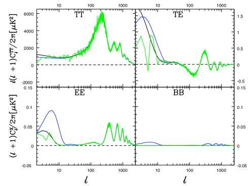
Figure 1: Angular power spectrum, $C_{\ell}$, of the Planck CMB reference sky, obtained from the reference sky spherical harmonics, $a_{\ell m}$, used to generate the signal of the 70 GHz observed map (green solid line); $C_{\ell}$ used to generate the Monte Carlo simulations for Phase 1 (blue solid line); $C_{\ell}$ used to generate the Monte Carlo simulations for Phase 2 (black solid line).

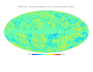
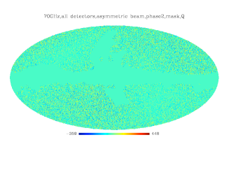
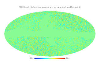
Figure 2: 70 GHz ($I$, $Q$, $U$) Stokes parameters of the observed map (from left to right hand side) for Phase 2b, generated with all detectors, convolved with the asymmetric beam and with mask (for galaxy plus missing pixels) applied.

3 XFaster Power spectrum and Likelihood estimator

3.1 XFaster Power spectrum estimator

XFaster (Contaldi et al. (2010); Netterfield et al (2002); Montroy et al (2006)) is an iterative, maximum likelihood, quadratic band power estimator (Bond Jaffe & Knox (2000); Knox (1999); Hamilton (1997); Tegmark (1997); Tegmark & de Oliveira-Costa (2001)) based on a diagonal approximation to the quadratic Fisher matrix estimator. It is a QML estimator formulated in the isotropic, diagonal approximation of the Master method (Hivon, Górski et al. (2002)).

It is common to expand the pixel temperature fluctuations (Stokes $I$), $T(\hat{{\bf{n}}})$, on the celestial sphere in terms of spherical harmonic functions, $Y_{\ell m}$, as

$$T(\hat{{\bf{n}}})=\sum_{\ell m}a_{\ell m}Y_{\ell m}(\hat{{\bf{n}}}),$$ (1)

with coefficients $a_{\ell m}$.

The maximum likelihood estimator (MLE) is based on a Gaussian assumption for the likelihood of the observed data (e.g., the pixel temperature, $T$, or its spherical harmonic transform $a_{\ell m}$):

$$L(\mathbf{d}|\mathbf{p})=\frac{1}{(2\pi)^{N/2}|\mathbf{C}|^{1/2}}\exp\left(-\frac{1}{2}\mathbf{d}\ \mathbf{C}^{-1}\mathbf{d}^{t}\right)$$ (2)

where $\mathbf{C}$ is the covariance of the data, and $\mathbf{p}$ is the set of model parameters. $\mathbf{C}(\mathbf{p})=\mathbf{S}(\mathbf{p})+\mathbf{N}$, where $\mathbf{S}$ is the sky signal and $\mathbf{N}$ is the noise. For single dish, full sky observations an isotropic signal is diagonal in the spherical harmonic space and can be described by an $m$-averaged power spectrum $C_{\ell}$ on each multipole, i.e., $S_{\ell m,\ell^{\prime}m^{\prime}}=\delta_{\ell\ell^{\prime}}\delta_{mm^{\prime}}C_{\ell}$. The noise is generally not diagonal.

All high-$\ell$ codes assume the data to be Gaussian distributed, however, they differ from XFaster on the devised unbiased frequentist power spectrum estimator. All algorithms form quadratic functions of the data. Pseudo-$C_{\ell}$ (PCL) codes estimate $C_{\ell}=\frac{1}{2\ell+1}\sum_{m=-\ell}^{m=\ell}\frac{|a_{\ell m}|^{2}}{4\pi}$ using fast spherical transforms. Example of such algorithms are all Master type codes [Hivon, Górski et al. (2002); Wandelt, Hivon & Górski (2001)] such as Romaster, cRomaster (Polenta et al. (2004)), Xpol (Tristram et al. (2005a, b)), and Crosspect (Ashdown et al. (2010)). Others calculate the angular correlation function $C(\theta)=\frac{1}{4\pi}\sum_{\ell\geq 2}(2\ell+1)C_{\ell}P_{\ell}(\cos{\theta})$ (where $P_{\ell}(\cos{\theta})$ is the Legendre polynomial and $\theta$ is an angular separation on the sky) using fast evaluation of the 2-point correlation function such as [Spice (Szapudi et al. (2001)), Polspice (Chon et al. (2003)], though this is achieved using fast spherical transforms. XFaster (Contaldi et al. (2010); Netterfield et al (2002); Montroy et al (2006), instead uses the Quadratic Maximum likelihood (QML) expression as derived below.

It can be shown that the$(\ell,m)$ space maximum likelihood solution for the power spectrum is given by (Bond Jaffe & Knox (2000); Hamilton (1997); Tegmark (1997); Tegmark & de Oliveira-Costa (2001)):

$$C_{\ell}=\frac{1}{2}\sum_{\ell^{\prime}}{\cal{F}}_{\ell\ell^{\prime}}^{-1}\>{\rm Tr}\left[\mathbf{C}^{-1}\frac{\partial\mathbf{S}}{\partial C_{\ell^{\prime}}}\ \mathbf{C}^{-1}(\mathbf{C^{obs}}-\mathbf{N})\right],$$ (3)

where $C_{\ell m,\ell^{\prime}m^{\prime}}^{obs}=a_{\ell m}^{obs}a_{\ell^{\prime}m^{\prime}}^{obs*}$ is the quadratic in the coefficients of the expansion of the observed map and ${\bf{\cal{F}}}$ is the Fisher information matrix for the $C_{\ell}$ parameters (= curvature matrix in the ensemble average limit), given by:

$${\cal{F}}_{\ell\ell^{\prime}}=\frac{1}{2}\>{\rm Tr}\left[\frac{\partial\mathbf{S}}{\partial C_{\ell}}\ \mathbf{C}^{-1}\frac{\partial\mathbf{S}}{\partial C_{\ell^{\prime}}}\ \mathbf{C}^{-1}\right].$$ (4)

An iterative scheme can be employed to reach the maximum likelihood estimate for the $C_{\ell}$: start with an initial guess; compute $\mathbf{\cal{F}}$; evaluate Eq 3. However, matrix operations become prohibitive for dimensions larger than a few thousand.

To circumvent this problem XFaster recasts the estimator in the isotropic, diagonal approximations of the Master methods (Hivon, Górski et al. (2002); Wandelt, Hivon & Górski (2001)) simplifying the calculations above. In this case the noise becomes a diagonalised Monte Carlo estimated bias and the signal is summed into bands to average down the correlations induced by any reduced sky coverage. In this case for a single mode, say temperature alone, the covariance of the observed cut-sky modes is approximated by

$$\tilde{C}_{\ell m,\ell^{\prime}m^{\prime}}=\delta_{\ell\ell^{\prime}}\delta_{mm^{\prime}}(\tilde{C}_{\ell}+\langle\tilde{N}_{\ell}\rangle),$$ (5)

where $\tilde{C}_{\ell}$ is the cut-sky model power spectrum. In our case the cut-sky power spectrum is parameterized through a set of deviations $q_{\ell}$ from a template full-sky ’shape’ spectrum $C_{\ell}^{(S)}$,

$$\tilde{C}_{\ell}=\sum_{\ell^{\prime}}K_{\ell\ell^{\prime}}B_{\ell^{\prime}}^{2}F_{\ell^{\prime}}C_{\ell^{\prime}}^{(S)}q_{\ell^{\prime}},$$ (6)

where $K_{\ell\ell^{\prime}}$ is the coupling matrix due to the cut sky observations (see section 3.1.1), $F_{\ell}$ is a transfer or filter function accounting for the effect of pre-filtering the data both in time and spatial domain (see section 3.1.2), and $B_{\ell}$ expresses the effect of a finite beam. For the case where the spectrum is parametrized in bands we consider band power deviations $q_{b}$

$$\tilde{C}_{\ell}=\sum_{b}q_{b}\tilde{C}_{b\ell}^{S}=\sum_{b}q_{b}\sum_{\ell^{\prime}}K_{\ell\ell^{\prime}}B_{\ell^{\prime}}^{2}F_{\ell^{\prime}}C_{\ell^{\prime}}^{S}\chi_{b}(\ell^{\prime}),$$ (7)

where $\chi_{b}(\ell)$ is a binning function. Assume for simplicity flat binning with $\chi_{b}(\ell)=1$ within the band and zero outside. The ML solution for the $q_{b}$ is

$$q_{b}=\frac{1}{2}\sum_{b^{\prime}}{\cal{F}}_{bb^{\prime}}^{-1}\sum_{\ell}(2\ell+1)g\frac{\tilde{C}_{b^{\prime}\ell}^{S}}{(\tilde{C}_{\ell}+\langle\tilde{N}_{\ell}\rangle)^{2}}(\tilde{C}_{\ell}^{obs}-\langle\tilde{N}_{\ell}\rangle),$$ (8)

where isotropy reduces the trace as Tr $\rightarrow$ $\sum_{\ell}(2\ell+1)g$, and $g$ describes the effective degrees of freedom in the maps (which may be reduced by additional weighting of the modes such as filtering or pixel weighting), and is related to the moments of the pixel weighting and the sky coverage, see Hivon, Górski et al. (2002), and it can be further impacted by the binning of the power spectrum:

$$g=f_{sky}\Delta\ell\frac{w_{2}^{2}}{w_{4}} {\rm where} f_{sky}w_{i}=\frac{1}{4\pi}\int_{4\pi}W^{i}(\hat{{\bf{n}}})d{\bf{n}}$$ (9)

where$\ W(\hat{{\bf{n}}})$ is the window or mask applied to the data, $f_{sky}w_{i}$ is the i-th moment of the arbitrary weighting scheme, and $\Delta\ell$ is the width of the multipole bins.
The expression for the Fisher matrix is now given by

$${\cal{F}}_{bb^{\prime}}=\frac{1}{2}\sum_{\ell}(2\ell+1)g\frac{\tilde{C}_{b\ell}^{S}\tilde{C}_{\ell b^{\prime}}^{S}}{(\tilde{C}_{\ell}+\langle\tilde{N}_{\ell}\rangle)^{2}},$$ (10)

For polarization sensitive observations the data include the $I$, $Q$, and $U$ Stokes parameters. As mentioned before, the $I$ map is expanded in terms of spherical harmonics while the $Q$ and $U$ maps are expanded in spin-2 spherical harmonics, ${}_{2}Y_{\ell m}$, to obtain E and B (grad-type or curl-type) polarization coefficients:

$$(Q\pm iU)(\hat{{\bf{n}}})=\sum_{\ell m}(a^{E}_{\ell m}\pm ia^{B}_{\ell m})_{\pm 2}Y_{\ell m}(\hat{{\bf{n}}})$$ (11)

There are six spectra representing the six independent elements of the $3\times 3$ covariance matrix of the $(\tilde{a}_{\ell m}^{T},\tilde{a}_{\ell m}^{E},\tilde{a}_{\ell m}^{B})$ vector:

$$\widetilde{C}_{\ell}^{TT} = \sum_{b}q_{b}^{TT}\widetilde{C}_{b\ell}^{(S)TT}+\widetilde{N}_{\ell}^{TT}$$ (12)

$$\widetilde{C}_{\ell}^{EE} = \sum_{b}(q_{b}^{EE}{{}_{+}\widetilde{C}}_{b\ell}^{(S)EE}+q_{b}^{BB}{{}_{-}\widetilde{C}}_{b\ell}^{(S)BB})+\widetilde{N}_{\ell}^{EE}$$ (13)

$$\widetilde{C}_{\ell}^{BB} = \sum_{b}(q_{b}^{BB}{{}_{+}\widetilde{C}}_{b\ell}^{(S)BB}+q_{b}^{EE}{{}_{-}\widetilde{C}}_{b\ell}^{(S)EE})+\widetilde{N}_{\ell}^{BB}$$ (14)

$$\widetilde{C}_{\ell}^{TE} = \sum_{b}q_{b}^{TE}\widetilde{C}_{b\ell}^{(S)TE}+\widetilde{N}_{\ell}^{TE}$$ (15)

$$\widetilde{C}_{\ell}^{TB} = \sum_{b}q_{b}^{TB}\widetilde{C}_{b\ell}^{(S)TB}+\widetilde{N}_{\ell}^{TB}$$ (16)

$$\widetilde{C}_{\ell}^{EB} = \sum_{b}q_{b}^{EB}\widetilde{C}_{b\ell}^{(S)EB}+\widetilde{N}_{\ell}^{EB}.$$ (17)

The template shape matrices are defined using the various coupling kernels for the different polarization types. The transfer functions are distinct for each polarization type:

$$\widetilde{C}_{b\ell}^{(S)TT} = \sum_{\ell^{\prime}}K_{\ell\ell^{\prime}}F_{\ell^{\prime}}^{TT}B_{\ell^{\prime}}^{2}C_{\ell^{\prime}}^{(S)TT}\chi_{b}(\ell),$$ (18)

$$\pm\widetilde{C}_{b\ell}^{(S)EE} = \sum_{\ell^{\prime}}{{}_{\pm}K}_{\ell\ell^{\prime}}F_{\ell^{\prime}}^{EE}B_{\ell^{\prime}}^{2}C_{\ell^{\prime}}^{(S)EE}\chi_{b}(\ell),$$ (19)

$$\pm\widetilde{C}_{b\ell}^{(S)BB} = \sum_{\ell^{\prime}}{{}_{\pm}K}_{\ell\ell^{\prime}}F_{\ell^{\prime}}^{BB}B_{\ell^{\prime}}^{2}C_{\ell^{\prime}}^{(S)BB}\chi_{b}(\ell),$$ (20)

$$\widetilde{C}_{b\ell}^{(S)TE} = \sum_{\ell^{\prime}}{{}_{\times}K}_{\ell\ell^{\prime}}F_{\ell^{\prime}}^{TE}B_{\ell^{\prime}}^{2}C_{\ell^{\prime}}^{(S)TE}\chi_{b}(\ell),$$ (21)

$$\widetilde{C}_{b\ell}^{(S)TB} = \sum_{\ell^{\prime}}{{}_{\times}K}_{\ell\ell^{\prime}}F_{\ell^{\prime}}^{TB}B_{\ell^{\prime}}^{2}C_{\ell^{\prime}}^{(S)TB}\chi_{b}(\ell),$$ (22)

$$\widetilde{C}_{b\ell}^{(S)EB} = \sum_{\ell^{\prime}}({{}_{+}K}_{\ell\ell^{\prime}}-{{}_{-}K}_{\ell\ell^{\prime}})F_{\ell^{\prime}}^{EB}B_{\ell^{\prime}}^{2}C_{\ell^{\prime}}^{(S)TB}\chi_{b}(\ell).$$ (23)

For simplicity the beam $B_{\ell}$ is assumed independent of polarization. (In principle, it could also be treated distinctly for each of the $T$, $E$, and $B$ modes.) The mask coupling kernels, $K_{\ell\ell^{\prime}}$, and the two additional polarization mask coupling kernels, ${}_{\pm}K_{\ell\ell^{\prime}}$, ${}_{\times}K_{\ell\ell^{\prime}}$ are defined in section 3.1.1.

Extending the above formalism to polarization, the XFaster estimator takes a matricial form, implemented trivially since the matrix $C$ is now block diagonal:
$\tilde{\mathbf{C}}\rightarrow diag(\tilde{\mathbf{D}}_{\ell_{min}},\tilde{\mathbf{D}}_{\ell_{min}+1},\dots,\tilde{\mathbf{D}}_{\ell_{max}})$, where each multipole’s covariance is a $3\times 3$ matrix:

$$\tilde{\mathbf{D}}_{\ell}=\left(\begin{array}[]{ccc}\tilde{C}_{\ell}^{TT}&\tilde{C}_{\ell}^{TE}&\tilde{C}_{\ell}^{TB}\\ \tilde{C}_{\ell}^{TE}&\tilde{C}_{\ell}^{EE}&\tilde{C}_{\ell}^{EB}\\ \tilde{C}_{\ell}^{TB}&\tilde{C}_{\ell}^{EB}&\tilde{C}_{\ell}^{BB}\\ \end{array}\right),$$ (24)

Similarly its inverse is a block diagonal of the inverses of $\tilde{\mathbf{D}}_{\ell}$ matrices and therefore simple to compute. The noise covariance matrix is also of this form, the $\tilde{N}_{\ell}^{XY}$ in each block diagonal is obtained by noise only Monte Carlo simulations. The band power deviations, $q_{b}$, take now the following form:

$$q_{b}=\frac{1}{2}\sum_{b^{\prime}}{\cal{F}}_{bb^{\prime}}^{-1}\sum_{\ell}(2\ell+1)g\>{\rm Tr}\left[{\tilde{\mathbf{D}}_{\ell}}^{-1}\frac{\partial\mathbf{\tilde{S}}}{\partial q_{b^{\prime}}}\ {\tilde{\mathbf{D}}_{\ell}}^{-1}\left({\tilde{\mathbf{D}}_{\ell}}^{obs}-\tilde{\mathbf{N}}_{\ell}\right)\right],$$ (25)

and the Fisher matrix is now given by:

$${\cal{F}}_{bb^{\prime}}=\frac{1}{2}\sum_{\ell}(2\ell+1)g\>{\rm Tr}\left[\tilde{\mathbf{D}}_{\ell}^{-1}\frac{\partial\mathbf{\tilde{S}}_{\ell}}{\partial q_{b}}\ \mathbf{\tilde{D}}_{\ell}^{-1}\frac{\partial\mathbf{\tilde{S}}_{\ell}}{\partial q_{b^{\prime}}}\right].$$ (26)

where the band index, b, spans bands in all polarization types. The derivatives of the signal matrices with respect to the deviations $q_{b}$ are given by:

$$\frac{\partial\mathbf{\tilde{S}}}{\partial q_{b}}|_{b::TT} = \left(\begin{array}[]{ccc}\tilde{C}_{b\ell}^{(S)TT}&0&0\\ 0&0&0\\ 0&0&0\\ \end{array}\right),\frac{\partial\mathbf{\tilde{S}}}{\partial q_{b}}|_{b::TE}=\left(\begin{array}[]{ccc}0&\tilde{C}_{b\ell}^{(S)TE}&0\\ \tilde{C}_{b\ell}^{(S)TE}&0&0\\ 0&0&0\\ \end{array}\right)$$ (33)

$$\frac{\partial\mathbf{\tilde{S}}}{\partial q_{b}}|_{b::EE} = \left(\begin{array}[]{ccc}0&0&0\\ 0&{{}_{+}\tilde{C}}_{b\ell}^{(S)EE}&0\\ 0&0&{{}_{-}\tilde{C}}_{b\ell}^{(S)EE}\\ \end{array}\right),\frac{\partial\mathbf{\tilde{S}}}{\partial q_{b}}|_{b::BB}=\left(\begin{array}[]{ccc}0&0&0\\ 0&{{}_{-}\tilde{C}}_{b\ell}^{(S)BB}&0\\ 0&0&{{}_{+}\tilde{C}}_{b\ell}^{(S)BB}\\ \end{array}\right)$$ (40)

$$\frac{\partial\mathbf{\tilde{S}}}{\partial q_{b}}|_{b::TB} = \left(\begin{array}[]{ccc}0&0&\tilde{C}_{b\ell}^{(S)TB}\\ 0&0&0\\ \tilde{C}_{b\ell}^{(S)TB}&0&0\\ \end{array}\right),\frac{\partial\mathbf{\tilde{S}}}{\partial q_{b}}|_{b::EB}=\left(\begin{array}[]{ccc}0&0&0\\ 0&0&\tilde{C}_{b\ell}^{(S)EB}\\ 0&\tilde{C}_{b\ell}^{(S)EB}&0\\ \end{array}\right).$$ (47)

These derivatives include contributions from both $(+)$ and $(-)$ kernels in the case EE and BB due to the geometrical leakage.

This estimator makes use of the Monte Carlo pseudo-$C_{\ell}$ formalism of Master methods to estimate noise bias and linear filter functions. It requires noise only Monte Carlo simulations to estimate the noise bias and signal only Monte Carlo simulations to estimate the filter function. Contrary to the conventional pseudo-$C_{\ell}$ based methods it does not requires signal+noise Monte Carlo simulations to estimate the uncertainty (variance) of the band powers, which is given by the Fisher matrix instead, a byproduct of the method. The Fisher matrix is computed self-consistently and runs over all band powers and polarizations. It takes into account all the correlations in the approximation used (coupling kernel and diagonal noise bias) and can therefore be used to compute, self-consistently, all ancillary information required in the estimation process, correlations, window functions, etc. In Figure 3 we plot the inverse of the fisher matrix for phase2, symmetric beam case. Note that the Fisher matrix is not diagonal.

Furthermore XFaster can estimate both auto-spectra and cross-spectra jointly, using the full covariance of the $a_{lm}$’s, via a multiple-map analysis.

As mentioned above, the noise is generally not diagonal. For Planck, the noise is white to good approximation at small angular scales; however, at large angular scales instrumental characteristics such as $1/f$ noise and thermal fluctuations combine with the scan strategy to produce significant off-diagonal correlations in the noise. Therefore, the XFaster approximation is not optimal at low-$\ell$ multipole range. We show in Sections 4.2 and 4.3 that XFaster is a very good approximation for $\ell>30$. We have no intention of using XFaster for Planck at low-$\ell$. Instead, we will combine one of the codes adequate at low-$\ell$ (listed in Section 1) with XFaster (or another high-$\ell$ estimator) into a hybrid estimator of the power spectrum that covers the entire multipole range.

Previous CMB experiments have customarily binned power spectra in multipole bands. The main reason for this is that it “enhances” the signal-to-noise ratio of the spectra. It also averages down correlations due to the reduced sky coverage at the same time as the coupling matrices due to the cut-sky attempt to correct the cut-sky effect. The XFaster power spectrum can be computed multipole by multipole, i.e., for each $\ell$, or in multipole bands. The band power spectra are given in Section 4.1. To estimate cosmological parameters we can use band power spectra with any high-$\ell$ likelihood approximation, e.g., with the Offfset Lognormal Bandpower likelihood presented in Rocha et al. (2010). However, as the XFaster likelihood is estimated multipole by multipole we can bypass the band power spectrum estimation step and estimate parameters directly from the maps (via its raw pseudo-$C_{\ell}$). Slices of the XFaster likelihood and parameter constraints are given in Section 4.2 and Section 4.3.

As kernels and transfer (filter) functions are an important ingredient in power spectrum estimation we describe next how they are computed within XFaster approach.

3.1.1 Kernels

The effect of masking the sky is to produce a power spectrum that is a linear combination of the full sky power spectrum multipoles on the sky. The coupling matrix due to the cut sky observations, $K_{\ell\ell^{\prime}}$, encodes this effect, it only depends on the geometry of the mask or window and is easily computable.
Considering a window function $W(\hat{{\bf{n}}})$, and ignoring the effects of beam convolution and filtering effects due to any pre-processing of the timelines, the ensemble averages of the cut-sky $\langle\widetilde{C}_{\ell}\rangle$ and the full-sky angular power spectrum $\langle C_{\ell}\rangle$ can be related by:

$$\langle\widetilde{C}_{\ell}\rangle=\sum_{\ell^{\prime}}K_{\ell\ell^{\prime}}\langle C_{\ell^{\prime}}\rangle,$$ (48)

with coupling matrix, $K_{\ell\ell^{\prime}}$ given by:

$$K_{\ell\ell^{\prime}}=\frac{2\ell^{\prime}+1}{4\pi}\sum_{\ell"}J(\ell,\ell^{\prime},\ell";0,0,0)^{2}W_{\ell"}^{2}$$ (49)

where $J(l,l^{\prime},l";0,0,0)={\left(\begin{array}[]{lcr}\ell&\ell^{\prime}&\ell^{\prime\prime}\\ 0&0&0\end{array}\right)}$ is the 3j symbol, and $W_{\ell}^{2}$ is the power spectrum of the window function $W(\hat{{\bf{n}}})$, that is $W_{\ell}^{2}=(2\ell+1){\cal{W}}_{\ell}$ with:

$${\cal{W}}_{\ell}=\frac{1}{2\ell+1}\sum_{m}|W_{\ell m}|^{2} {\rm and} W_{\ell m}=\int d{\bf{n}}W(\hat{{\bf{n}}})Y^{*}_{\ell,m}(\hat{{\bf{n}}})$$ (50)

$${\cal{W}}_{0}=W_{0}^{2}=4\pi f_{sky}^{2}w_{1}^{2} {\rm and} \sum_{\ell\geq 0}W_{\ell}^{2}=\sum_{\ell\geq 0}(2\ell+1){\cal{W}}_{\ell}=4\pi f_{sky}w_{2}$$ (51)

Hence

$$K_{\ell\ell^{\prime}}=\frac{2\ell^{\prime}+1}{4\pi}\sum_{\ell^{\prime\prime}}(2\ell^{\prime\prime}+1)\mathcal{W}_{\ell^{\prime\prime}}{\left(\begin{array}[]{lcr}\ell&\ell^{\prime}&\ell^{\prime\prime}\\ 0&0&0\end{array}\right)}^{2}$$ (52)

Extending the above to polarized data we consider the additional polarization mask coupling kernels defined as follows:

$${}_{\pm}K_{\ell\ell^{\prime}} = \frac{2\ell^{\prime}+1}{16\pi}\sum_{L}(2L+1)\mathcal{W}_{L}{\left(\begin{array}[]{lcr}\ell&\ell^{\prime}&L\\ 2&-2&0\end{array}\right)}^{2}\left(1\pm(-1)^{\ell+\ell^{\prime}+L}\right)$$ (55)

$${}_{\times}K_{\ell\ell^{\prime}} = \frac{2\ell^{\prime}+1}{8\pi}\sum_{L}(2L+1)\mathcal{W}_{L}{\left(\begin{array}[]{lcr}\ell&\ell^{\prime}&L\\ 2&-2&0\end{array}\right)}{\left(\begin{array}[]{lcr}\ell&\ell^{\prime}&L\\ 0&0&0\end{array}\right)}\left(1+(-1)^{\ell+\ell^{\prime}+L}\right)$$ (60)

These kernels account for the leakage of power between E and B modes induced by the usage of the full-sky ${}_{\pm 2}Y_{\ell m}(\hat{{\bf{n}}})$ basis on a cut-sky.

In Figure 4 we plot the masks for temperature and polarization used in Phase 2 (see section 2).

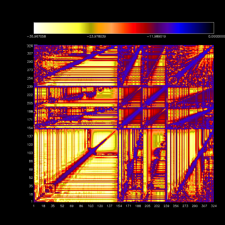
Figure 3: Logarithm of the absolute value of the ‘normalized’ (ie set to 1 at the maximum value) inverse of the Fisher matrix (covariance matrix) for phase2, symmetric beam case. TT, EE, BB and TE modes are displayed sequentially from bottom left-hand side corner to the upper right-hand side corner along the diagonal.

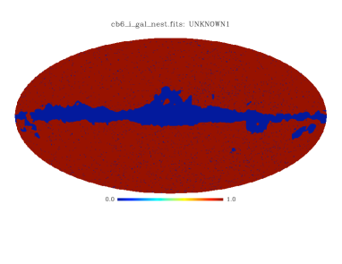
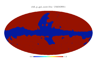
Figure 4: Mask for Temperature (left hand side) and polarization (right hand side) used in Phase 2. The $f_{\rm sky}\simeq 0.85$ for Temperature and $f_{\rm sky}\simeq 0.73$ for Polarization.

3.1.2 Transfer or Filter functions

To compute $F_{\ell}$ we start with Eq. 7 for the signal only Monte Carlo simulations, and as $F_{\ell}$ is assumed to be smooth over each multipole bin we move $F_{\ell}$ out of the summation for each bin $b$, to get:

$$\tilde{C}_{\ell}=\sum_{b}q_{b}\tilde{C}_{b\ell}^{S}=\sum_{b}q_{b}F_{b}\sum_{\ell^{\prime}}K_{\ell\ell^{\prime}}B_{\ell^{\prime}}^{2}C_{\ell^{\prime}}^{S}\chi_{b}(\ell^{\prime})$$ (61)

and proceed with the iterative scheme as one would to estimate $q_{b}$ but now we estimate the transfer function, $F_{b}$ instead. This is achieved by fixing $q_{b}=1$, varying $F_{b}$ and considering the signal only Monte Carlo simulations.

$$F_{b}=\frac{1}{2}\sum_{b^{\prime}}{\cal{F}}_{bb^{\prime}}^{-1}\sum_{\ell}(2\ell+1)g\frac{\tilde{C}_{b^{\prime}\ell}^{S}}{(\tilde{C}_{\ell}+\langle\tilde{N}_{\ell}\rangle)^{2}}\langle\tilde{S}_{\ell}\rangle$$ (62)

where $\langle\tilde{S}_{\ell}\rangle$ is the average of the signal only Monte Carlo simulations.

Extending to polarization we have:

$$F_{b}=\frac{1}{2}\sum_{b^{\prime}}{\cal{F}}_{bb^{\prime}}^{-1}\sum_{\ell}(2\ell+1)gTr\left[{\tilde{\mathbf{D}}_{\ell}}^{-1}\frac{\partial\mathbf{\tilde{S}}}{\partial q_{b^{\prime}}}\ {\tilde{\mathbf{D}}_{\ell}}^{-1}\langle\tilde{\mathbf{S}}_{\ell}\rangle\right],$$ (63)

3.2 XFaster likelihood estimator

A very attractive feature of the XFaster power spectrum estimator is that is naturally provides a likelihood, i.e., the Probability of the observed cut sky data given the model. In the XFaster approximation, considering only one mode (say Temperature alone), the likelihood takes the following form, up to a constant (where $\tilde{A}$ means $A$ estimated on the cut-sky):

$$\ln L=-\frac{1}{2}\sum_{\ell}g(2\ell+1)\left(\frac{\tilde{C_{\ell}}^{obs}}{\left(\tilde{C_{\ell}}+\left<\tilde{N_{\ell}}\right>\right)}+\ln\left(\tilde{C_{\ell}}+\left<\tilde{N_{\ell}}\right>\right)\right)$$ (64)

where $\tilde{C}_{\ell}$ is the cut-sky model power spectrum given by Eq. 7 in Section 3.1, for the case where the spectrum is parametrized in bands we consider band power deviations $q_{b}$.

Extending to Temperature and Polarization we have:

$$\ln L=-\frac{1}{2}\sum_{\ell}g(2\ell+1)\left(Tr\left({\tilde{\mathbf{D}_{\ell}^{obs}}}{\left(\tilde{\mathbf{D}_{\ell}}+\left<\tilde{\mathbf{N}_{\ell}}\right>\right)^{-1}}\right)+\ln\left|\tilde{\mathbf{D}_{\ell}}+\left<\tilde{\mathbf{N}_{\ell}}\right>\right|\right)$$ (65)

Where $\tilde{\mathbf{N}_{\ell}}$ and $\tilde{\mathbf{D}_{\ell}}$ are given in section 3.1.

An interesting point to note is that XFaster likelihood follows intuitively from the usual full-sky ideal case exact likelihood (an inverse Gamma distribution for temperature alone and an inverse Wishart distribution for temperature + polarization (see e.g., Rocha et al. (2010)).

Here we use one dimensional slices as an approximation to investigate the non-Gaussianity of the likelihood. One samples in each deviation $q_{b}$ direction individually around the maximum likelihood solution $q_{b}^{*}$. This approximation is adequate if the band powers are not heavily correlated. Note that the likelihood slices are estimated along the bands and not along each $\ell$, and hence will be affected by the binning procedure. To compare XFaster likelihood to other approximations we make use of slices computed along the bandpower spectrum deviations, $q_{b}$. Such likelihood slices for the 70 GHz observed map are plotted in Section 4.2.

When estimating parameters with XFaster likelihood, by default estimated multipole by multipole, we do not make use of the bandpower spectra. It is in this sense that XFaster likelihood allows to go straight from the maps to parameters bypassing the band power spectrum step. It only requires the raw pseudo-$C_{\ell}$ of the observations plus the kernel and transfer function to relate the cut-sky pseudo-$C_{\ell}$ to the full-sky $C_{\ell}$.

3.2.1 Window functions

To compare the theoretical power spectrum to the observed power spectrum and to estimate parameters, we must construct an operator for obtaining theoretical bandpowers from model power spectra $C_{\ell}^{T}$. Following Bond Jaffe & Knox (2000) we define a logarithmic integral

$$\mathcal{I}[f_{\ell}]=\sum_{\ell}\frac{\ell+\frac{1}{2}}{\ell(\ell+1)}f_{\ell},$$ (66)

which is used to calculate the expectation values for the deviations $q_{b}$(when a shape model, $C_{\ell}^{S}$ is considered), or bandpowers $C_{b}$ (when $C_{\ell}^{S}$ is assumed to be flat).

$$\langle q_{b}\rangle=\frac{\mathcal{I}\left[W_{\ell}^{b}\mathcal{C}_{\ell}\right]}{\mathcal{I}\left[W_{\ell}^{b}\mathcal{C}_{\ell}^{(S)}\right]}\qquad\langle C_{b}\rangle=\frac{\mathcal{I}\left[W_{\ell}^{b}\mathcal{C}_{\ell}\right]}{\mathcal{I}\left[W_{\ell}^{b}\right]},$$ (67)

where $W_{\ell}^{b}$ is the band power window function, and $\mathcal{C}^{(S)}=\ell(\ell+1)C_{\ell}^{(S)}/2\pi$.

We define normalized window functions to be

$$\mathcal{I}\left[W_{\ell}^{b}\mathcal{C}_{\ell}^{(S)}\right]=1.$$ (68)

By taking the ensemble average limit of Eq.  (8) and using the fact that

$$\langle(\widetilde{C}_{\ell}^{obs}-\widetilde{N}_{\ell})\rangle\rightarrow\widetilde{C}_{\ell}$$ (69)

we obtain

$$W_{\ell}^{b}=\frac{4\pi}{(2\ell+1)}\sum_{b^{\prime}}{\cal{F}}_{bb^{\prime}}^{-1}\sum_{\ell^{\prime}}g(2\ell^{\prime}+1)\frac{\widetilde{C}_{b^{\prime}\ell^{\prime}}^{(S)}}{(\widetilde{C}_{\ell^{\prime}}+\langle\widetilde{N}_{\ell^{\prime}}\rangle)^{2}}K_{\ell\ell^{\prime}}F_{\ell}B_{\ell}^{2}.$$ (70)

Extending to polarization:

$$W_{\ell}^{b}=\frac{4\pi}{(2\ell+1)}\sum_{b^{\prime}}{\cal{F}}_{bb^{\prime}}^{-1}\sum_{\ell^{\prime}}g(2\ell^{\prime}+1){\rm Tr}\left[\mathbf{W}_{b^{\prime}\ell^{\prime}}\mathbf{K}_{\ell^{\prime}}\right]$$ (71)

where $\mathbf{W}_{b\ell}={\tilde{\mathbf{D}}_{\ell}}^{-1}\frac{\partial\mathbf{\tilde{S}}}{\partial q_{b}}{\tilde{\mathbf{D}}_{\ell}}^{-1}$, and $\mathbf{K}_{\ell}$ gives the cut-sky response to the individual full-sky multipoles:

$$\mathbf{K}_{\ell}=\left(\begin{array}[]{ccc}K_{\ell^{\prime}\ell}F_{\ell}^{TT}B_{\ell}^{2}&{}_{\times}K_{\ell^{\prime}\ell}F_{\ell}^{TE}B_{\ell}^{2}&{}_{\times}K_{\ell^{\prime}\ell}F_{\ell}^{TB}B_{\ell}^{2}\\ {}_{\times}K_{\ell^{\prime}\ell}F_{\ell}^{TE}B_{\ell}^{2}&{}_{+}K_{\ell^{\prime}\ell}F_{\ell}^{EE}B_{\ell}^{2}+_{-}K_{\ell^{\prime}\ell}F_{\ell}^{BB}B_{\ell}^{2}&\left({}_{+}K_{\ell^{\prime}\ell}-_{-}K_{\ell^{\prime}\ell}\right)F_{\ell}^{EB}B_{\ell}^{2}\\ {}_{\times}K_{\ell^{\prime}\ell}F_{\ell}^{TB}B_{\ell}^{2}&\left({}_{+}K_{\ell^{\prime}\ell}-_{-}K_{\ell^{\prime}\ell}\right)F_{\ell}^{EB}B_{\ell}^{2}&{}_{+}K_{\ell^{\prime}\ell}F_{\ell}^{BB}B_{\ell}^{2}+_{-}K_{\ell^{\prime}\ell}F_{\ell}^{EE}B_{\ell}^{2}\\ \end{array}\right).$$ (72)

These window functions were used and compared to the top hat window functions in Rocha et al. (2010) using the XFaster bandpower spectra and the Offset Lognormal Bandpower likelihood. However as the XFaster likelihood is estimated for each $\ell$, a comparison of observed to theoretical power spectrum does not make use of such windows. Instead the raw pseudo-$C_{\ell}$ of the observations, the kernels, and transfer or filter functions are all that is required for such comparison (see section 4.3).

3.3 The algorithm

The power spectrum is estimated by the following procedure:

• Generate Monte Carlo simulations of time-ordered data (TOD) for both signal and noise. The noise must have the same characteristics as the observed data, and in practice must be determined from the observed data. The simulated signal, on the other hand, can be almost anything, as it is simply a tracer of the effects of time and spatial domain filtering in the process, and used to calculate the transfer function $F_{\ell}$. In practice, it is convenient to use an approximate model of the CMB to generate the signal.

• Make maps of the TOD using the same mapmaking code as used for the observations.

• Estimate the pseudo-$C_{\ell}$ spectra and the spherical harmonic coefficients $a_{\ell m}$ from the signal only maps to get the transfer function $F_{\ell}$.

• Estimate the pseudo-$C_{\ell}$ spectra from the noise only maps to compute the noise bias $\langle\tilde{N}_{\ell}\rangle$. The pseudo-spectra can be computed with anafast of HEALPix package (Górski et al. (2005)) when the masks are the same for temperature and polarization, otherwise we use a specific code from the suite of XFaster modules.

• Iterate Equations 8 and 10 to obtain an estimate of $q_{b}$. In the diagonal, isotropic approximation of XFaster, the computational cost of the iterative estimator is very small compared with that of the TOD generation and map-making stages.

• The iterative estimator yields the Fisher information matrix automatically. An estimate of the band power covariance is given by $\mathbf{\cal{F}}^{-1}$, therefore we automatically get the uncertainty on the estimator.

Large ensembles of signal+noise simulations are not required to estimate the band power covariance matrix as in the Master procedure, cutting the cost of Monte Carlo simulations by $1/3$. Furthermore the covariance is not biased by an assumed model (which at very least requires the Master procedure to be run twice to be close to unbiased errors).

As mentioned in Section 3.1 XFaster can estimate both auto-spectra and cross-spectra jointly, using the full covariance of the $a_{lm}$, via a multiple-map analysis.

3.3.1 Computational scaling

The overall scaling for XFaster without accounting for the signal and noise Monte Carlo simulations should go as $\ell_{max}(n_{maps}\times n_{pol})^{3}$ for the internal Fisher calculation, where $n_{pol}$ is either 1 or 3, with a further scaling of $(n_{bins})^{3}$ for the outer iteration step.

Currently the code is not optimised for speed. It could be sped up substantially by parallelizing the Fisher computation and would then scale linearly with number of processors.

Approximate times for a single CPU for Phase2, with CTP binning and using 30 Fisher iterations are as follows:

• $a_{lm}$ and $C_{\ell}$ from the 100 Monte Carlo simulated maps: $\simeq 8$ hours ($\simeq$ 5 minutes each)

• kernel: 30 minutes

• transfer function: 30 minutes (less if one relaxes the binning)

• power spectrum: 1 hour

• average mode to check for possible bias: 15–20 minutes

4 Results

4.1 Results: Power spectrum

We estimated transfer (filter) functions, kernels, and the power spectrum for the observed map described in Section 2. We also computed the power spectrum for the average of the signal+noise simulated maps. This average mode run checks for possible biases of the power spectrum estimator itself. In principle, the estimator if unbiased should follow closely the input signal $C_{\ell}$ model used to generate the signal simulations.

Figure 5 shows the power spectra estimated for the observed map for Phase 1 and Phase 2 and their $1\sigma$ error bars. The power spectra recover accurately the input power spectrum in the middle range of multipoles, $30\leq\ell\leq 1000$. At high-$\ell$ ( $\ell\geq 1000$), they are impacted by the noise. At low-$\ell$, as the large scale structure of the observed map is a WMAP constrained realization, the estimated power spectrum is not necessarily consistent with, and exhibits a dispersion around, the best-fit spectrum.  Comparing the power spectra for the diverse phases we conclude that the cut-sky anisotropic noise case (Phase 1b) exhibits slightly greater uncertainties and slightly larger multipole to multipole variations at low-$\ell$ than the full-sky, isotropic noise case (Phase 1a). This is expected, as the cut-sky will induce correlations at low-$\ell$. The kernels correct these correlations; however, there is still a small residual dispersion. On the other hand the anisotropic noise will enhance the overall white noise level increasing the power spectrum uncertainty. For Phase 2 the dispersion of the power spectrum and uncertainties at low-$\ell$ are enhanced due to the residuals of correlated $1/f$ noise. As in Figure 5, the power spectrum for Phase 1 is estimated from maps generated with a smaller number of detectors (four) than those for Phase 2 (twelve), and is therefore noisier by a factor of the order $\frac{1}{\sqrt{3}}$. Therefore the error bars of the Phase 2 power spectrum are smaller than those of Phase 1. The right thing to do though is to compare the power spectra estimated for the same number of detectors. In Figure 6 we compare the power spectra for Phase 1a (middle plot) and Phase 2 (right hand side), both estimated on maps generated with all twelve detectors. As expected, the uncertainty for Phase 1a is now smaller than that of Phase 2.

The power spectra for Phase 2 for both the symmetric and asymmetric beams are highly consistent. Therefore we conclude that the beam asymmetry is reasonably well-handled by XFaster (see Section 4.1.1 for more details).

Figure 7 shows the transfer functions for Phase 1 and Phase 2. Except for Phase 2b, all are close to $1$. This is expected, as we do not pre-filter the TOD and the only effect at low-${\ell}$ is that due to the mapmaking step and to the limited number of Monte Carlos of the signal maps available. This means there is remaining sample variance on the large-scales although not very significant. We included the transfer function estimates because they are an integral part of the method and in real life they will not be equal to 1. However to investigate and show that the significance of these small departures from 1 are not significant we estimated the power spectrum with transfer function=1 as plotted in Figure 6. We also highlighted the fact that the transfer functions are estimated consistently between polarization types (i.e. taking into account cross-correlation between polarization modes in any realization). Note that in this work we did not take into account the remaining MC error in the transfer function in the final estimate of the power spectrum since any production run used in the real case will include many more realizations than used in this work (they could be easily included by adding to the final Fisher matrix if needed). However, for the asymmetric beam case the transfer function exhibits an upturn at high-$\ell$. This upturn tries to correct the mismatch between the ’real’ asymmetric beam and our assumed symmetric beam (as discussed in Section 4.1.1). As the input BB power spectrum model of the signal Monte Carlo simulations for Phase 2 is set to zero, we cannot constrain the BB transfer function. The transfer function obtained reflects the inadequacy of the input model and hence is close to zero. When estimating the power spectrum we replace the BB transfer function by the EE transfer function.

Figure 8 shows the power spectrum estimated for the average mode run. Whereas Figure 9 shows the difference between the power spectrum obtained for the average mode run (with error bars) and the fiducial model, $C_{\ell}$, used as input, for phase2, asymmetric beam case. The stepwise decreases of the amplitude of the error bars are caused by the changes of the $C_{\ell}$’s bins size. These plots show that the power spectrum follows the input signal $C_{\ell}$, confirming that XFaster is an unbiased estimator. These results were obtained using 100 Monte Carlo simulations. Considering 500 simulations for phase1a the small departures of the transfer function from 1 reduces slightly. Due to computational constraints this was not feasible for phase2. However increases in computational capability over time make it now possible to generate thousands of simulations. Results for 143GHz channel will be presented in our upcoming papers Rocha et al. (2010); Ashdown et al. (2010).

Figure 10 shows a variation of the above plots in which the BB power spectrum replaces the noise Monte Carlo simulations. These plots show that whenever the noise Monte Carlo simulations exhibit issues in the sense that they do not reflect accurately the noise characteristics of the observations, replacing them by the BB power spectrum is an adequate procedure, as for Planck at 70 GHz the BB power spectrum is mostly dominated by noise.

The power spectrum estimated for the observed map has been compared with those from several other methods (Ashdown et al. (2010)). To further assess the power spectrum estimator we propagated this analysis to cosmological parameter estimation using the new XFaster likelihood as described in Section 4.3

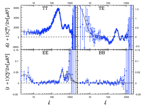
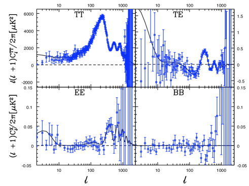
Figure 5: Power spectrum estimated with XFaster and $1\sigma$ error bars. Top row—Phase 1a (left hand side) and Phase 1b (right hand side) for map generated with a quadruplet of detectors. Bottom row—Phase 2a symmetric beam (left hand side) and Phase 2b asymmetric beam (right hand side) for map generated with all twelve detectors,. The plot displays the estimated power spectrum (blue) of the observed map, overplotted with the $C_{\ell}$ fiducial model used as input in Phase 2 signal simulations, first year WMAP+CBI+ACBAR best fit model (black).

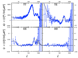
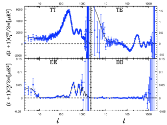
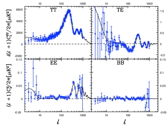
Figure 6: Power spectrum estimated with XFaster and $1\sigma$ error bars, considering transfer function=1 for Phase 1a, for map generated with a quadruplet of detectors (left hand side), with all twelve detectors (middle) and for Phase 2a, map generated with all twelve detectors and convolved with a symmetric beam (right hand side). This plot displays the estimated power spectrum (blue) of the observed map, overplotted with the $C_{\ell}$ fiducial model used as input in Phase 2 signal simulations, first year WMAP+CBI+ACBAR best fit model (black).

Figure 7: Transfer Function: Top row - for Phase 1a (left hand side) and Phase 1b (right hand side); Bottom row - for Phase 2a symmetric beam (left hand side) and Phase 2b asymmetric beam (right hand side).

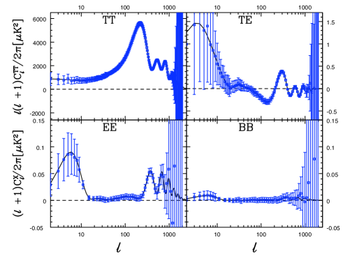
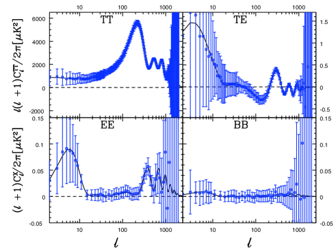
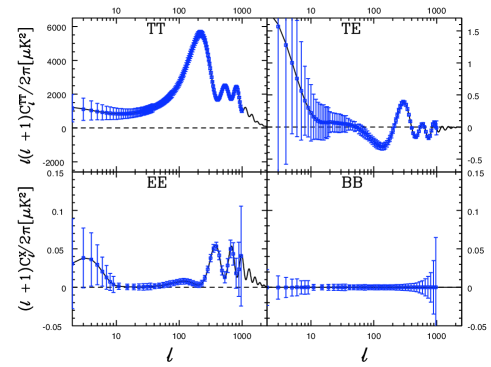
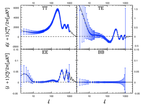
Figure 8: Power spectrum obtained with XFaster in average mode, meaning that we replaced the observed map by the average of the signal+noise simulated maps (blue). Top row—Phase 1a (left hand side) and Phase 1b (right hand side) for map generated with a quadruplet of detectors. Bottom row—Phase 2a symmetric beam (left hand side) and Phase 2b asymmetric beam (right hand side) for map generated with all twelve detectors, overplotted with the $C_{\ell}$ fiducial model used as input in our Phase 1 signal simulations, first year WMAP best fit model (black) for Phase 1 and first year WMAP+CBI+ACBAR best fit model (black) for Phase 2. It serves the purpose of checking for possible biases of the power spectrum estimator—in principle the power spectrum estimated in average mode should follow closely the input signal $C_{\ell}$ model used to generate the signal simulations (black).

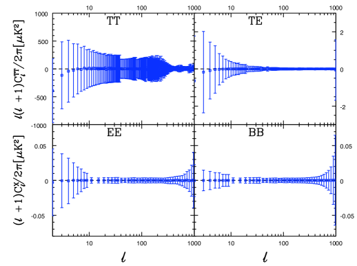
Figure 9: Difference of the power spectrum obtained with XFaster in average mode, (meaning that we replaced the observed map by the average of the signal+noise simulated maps) and the $C_{\ell}$ fiducial model used as input (first year WMAP+CBI+ACBAR best fit model), for phase2, asymmetric beam case. The stepwise decreases of the amplitude of the error bars are caused by the changes of the $C_{\ell}$ bins size.

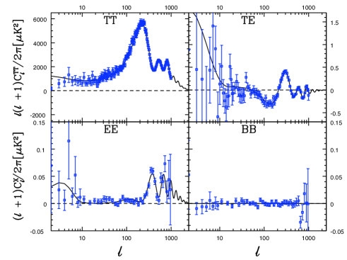
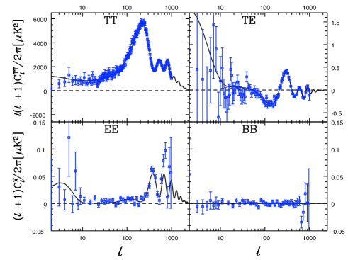
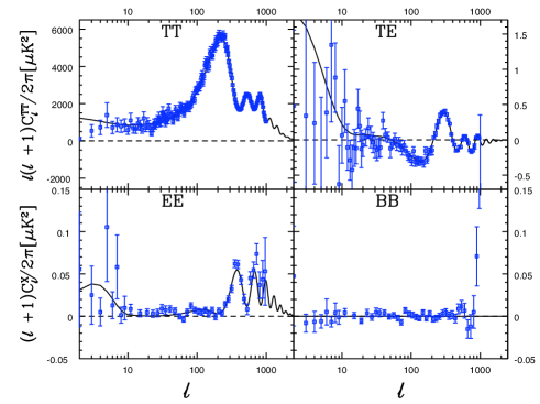
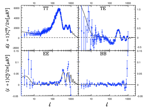
Figure 10: Power spectrum estimated with XFaster and $1\sigma$ error bars for Phase 2, for map generated with all twelve detectors, for symmetric (top row) and asymmetric (bottom row) beams. Left hand side plot displays the estimated power spectrum (blue) if the observed map, overplotted is the $C_{\ell}$ fiducial model used as input in our signal simulations, first year WMAP+CBI+ACBAR best fit model (black); Right hand side plot displays the estimated power spectrum with noise Monte Carlo simulations replaced by the BB power spectrum.

4.1.1 Symmetric and asymmetric beams

To study the impact of beam asymmetries on power spectrum and cosmological parameter estimation, we took a minimal, non-informative approach. When computing the power spectrum for the observed maps convolved with symmetric and asymmetric beams we assumed a FWHM = 14^′ symmetric beam for both cases.

We started by investigating the effect of this assumption on the shape of the transfer function, $F_{\ell}$, in Equations 6 and  7, or $F_{b}$ in Equations 61, 62, and 63. In effect we compute not only $F_{\ell}$, but also $F_{\ell}\delta{b_{\ell}}$, where $\delta{b_{\ell}}$ is the correction to the beam transfer function $B_{\ell}$. This correction arises from assuming a symmetric beam when estimating the power spectrum of an observed map that in fact has been convolved with an asymmetric beam. Call this function the generalized transfer function, $(BF)_{\ell}$. As mentioned in Section 4.1, since we do not pre-filter the TOD the only effect at low-${\ell}$ is that due to the mapmaking step. Therefore the transfer function should be very close to unity, particularly for the symmetric beam. Figure 13 shows $(BF)_{\ell}$ for both cases. For the symmetric case this function is very close to $1$ as expected, with tiny oscillations around $1$ at low-${\ell}$ consistent with our expectations. Apart from the transfer function for the BB mode for phase2 which is close to zero. Since the input BB power spectrum model of the signal Monte Carlo simulations for phase2 is set to zero we cannot constrain the transfer function for the BB mode. We resort to using the transfer function for the EE mode to estimate the BB power spectrum instead.

The symmetric and asymmetric $(BF)_{\ell}$ differ. In the asymmetric case, the function exhibits an upturn at high $\ell$. This upturn tries to correct the mismatch between the ’real’ asymmetric beam and our assumption. Hence the resulting power spectrum is pretty consistent for both cases, as shown in Figure 11. Considering the input symmetric beam with FWHM = 14^′  and the estimated FWHM$\simeq 13{{}^{\scriptscriptstyle\prime}}$ for the asymmetric beam, this effect should be approximately $(14/13)^{2}$, although anisotropic pixel filtering will add an extra component of aliasing in the maps at high-${\ell}$.

Although the power spectra look consistent, the parameter estimation shows departures of the order of $\sigma/2$ for some of the parameters, as shown in Section 4.3. To investigate this further we enhanced the previous plot into Figure 12. Though there is very good agreement between the two power spectra, there is still a slight bias for the asymmetric beam case. This bias is consistent with the small differences in the estimated parameters, in particular for $n_{s}$, $\sigma_{8}$ and $\log[10^{10}A_{s}]$ (see Section 4.3).

Next we study the impact of using two different sets of Monte Carlo simulations on the estimation of the power spectrum for the asymmetric beam case, Phase 2b. One set is the Monte Carlo simulations for the symmetric beam (Phase 2a) and the other the correct Monte Carlo simulations for the asymmetric beam (Phase 2b) study. On the right hand side of Figure 11 we plot the power spectrum estimated using both sets of simulations. The power spectrum of the observed map of Phase 2b (convolved with an asymmetric beam), estimated using the Monte Carlo simulations for Phase 2a (convolved with the symmetric beam), is biased high at high-$\ell$, as expected.

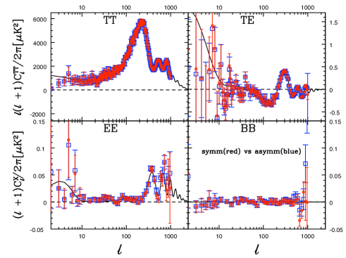
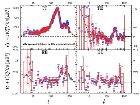
Figure 11: Power spectrum estimated with XFaster and $1\sigma$ error bars for Phase 2. The lefthand plot displays the power spectrum for a map generated with all twelve detectors, for both symmetric (red) and asymmetric (blue) beam cases. For both runs a symmetric beam with FWHM = 14^′ is assumed. The resulting power spectra are highly consistent, the compensation is achieved via the generalized transfer function $(BF)_{\ell}$. The righthand plot displays the power spectrum estimated for map generated with a quadruplet of detectors, with two different sets of Monte Carlo simulations. In one case we use the Monte Carlo simulations convolved with the symmetric beam (blue); in the other we use the correct Monte Carlo simulations convolved with the asymmetric beam (red). Making use of the Monte Carlo simulations for the symmetric case gives rise to a bias high at high-$\ell$.

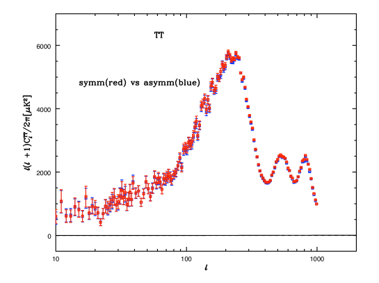
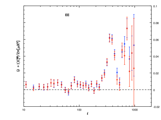
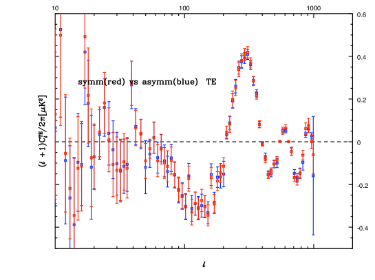
Figure 12: Power spectrum estimated with XFaster and $1\sigma$ error bars for Phase 2, for map generated with all twelve detectors, for both symmetric (red) and asymmetric (blue) beam cases. For both runs a symmetric beam with FWHM = 14^′ is assumed, the resulting power spectrum is consistent with each other, the mismatch is corrected via the generalized transfer function, $(BF)_{\ell}$. There is still a slight bias for the asymmetric case in agreement with the small differences of the estimated cosmological parameters (see section 4.3).

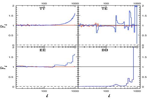
Figure 13: Comparison of transfer (filter) functions for Phase 2, for map generated with all twelve detectors, for symmetric beam (red solid line) and for asymmetric beam case (blue solid line).

4.2 Results: Likelihood

Following Section 3.2 we use one dimensional slices as an approximation to investigate the Non-Gaussianity of the likelihood, sampling in each $q_{b}$ direction around the maximum likelihood solution $q_{b}^{*}$. This approximation is adequate if the band powers are not heavily correlated. Note that the likelihood slices are estimated along the $q_{b}$ band power deviations and not along the $q_{\ell}$ power deviations for each multipole $\ell$, and hence are affected by the binning procedure. These slices are plotted in Figures 14, 15, 16, 17.

Figures 14 and 15 compare the XFaster likelihood to four other likelihood approximations, Gaussian, Lognormal, Offset Lognormal, and Equal Variance (Bond Jaffe & Knox (2000); Rocha et al. (2010)). A thorough account of these likelihood approximations is given elsewhere (see for instance Rocha et al. (2010)), here we give a brief account of their definitions. In what follows $\hat{C}$ means the measured or observed quantity $C$.
The Gaussian approximation, (Bond Jaffe & Knox (2000)), is a likelihood that is Gaussian in the $\hat{C}_{\ell}$ i.e.

$$P(\hat{\mn@boldsymbol{C}}|\mn@boldsymbol{C})\propto\exp\left\{-\frac{1}{2}(\hat{\mn@boldsymbol{C}}-\mn@boldsymbol{C})^{T}\mn@boldsymbol{S}^{-1}(\hat{\mn@boldsymbol{C}}-\mn@boldsymbol{C})\right\}$$ (73)

where $\mn@boldsymbol{C}$ is a vector of $C_{\ell}$ values (and similarly $\mn@boldsymbol{\hat{C}}$) and $\mn@boldsymbol{S}^{-1}$ is the inverse signal covariance matrix.
The Offset Lognormal likelihood, (Bond Jaffe & Knox (2000)), is given by:

$$P_{LN}(\hat{\mn@boldsymbol{C}}|\mn@boldsymbol{C})\propto\exp\left\{-\frac{1}{2}(\hat{\mn@boldsymbol{z}}-\mn@boldsymbol{z})^{T}\mn@boldsymbol{M}(\hat{\mn@boldsymbol{z}}-\mn@boldsymbol{z})\right\},$$ (74)

where $z_{\ell}=\ln(C_{\ell}+x_{\ell})$ and the matrix $\mn@boldsymbol{M}$ is related to the inverse covariance matrix by

$$M_{\ell\ell^{\prime}}=(C_{\ell}+x_{\ell})S^{-1}_{\ell\ell^{\prime}}(C_{\ell}^{\prime}+x_{\ell}^{\prime})$$ (75)

(The offset factors $x_{\ell}$ are simply a function of the noise and beam of the experiment.)
The Equal Variance likelihood, (Bond Jaffe & Knox (2000)) is given by:

$$\ln L=-\frac{1}{2}G\left[e^{-(z-\hat{z})}-\left(1-(z-\hat{z})\right)\right]$$ (76)

with

$$z=\ln\left(q_{b}+q_{b}^{N}\right)$$ (77)

and

$$G=\left[e^{-\sigma_{z}}-(1-\sigma_{z})\right]^{-1} {\rm with} \sigma_{z}=\frac{\sqrt{{\cal{F}}_{bb^{\prime}}^{-1}}}{(q_{b}+q_{b}^{N})}$$ (78)

The noise offset $q_{b}^{N}$ is estimated using the equation of the maximum likelihood solution for the $q_{b}$ replacing the observed map with the average of the noise Monte Carlo simulation power spectra $\left<\tilde{N_{\ell}}\right>$.

We use the values of the power spectrum and Fisher errors estimated with XFaster for Phase 2b (map generated with all twelve detectors and convolved with the asymmetric beam). As we are primarily interested in the shape of the likelihoods not on the actual value of the peaks, the comparison of the slices is done assuming they all peak at the same value, ie we use the band power specta estimated with XFaster and the functional shape of the other high-l likelihoods. This is the same to say that we first compute the band power spectra and apply the functional forms whereas XFaster likelihood slices are computed when estimating the band-power spectra. Figure 14 shows temperature slices of the XFaster joint temperature and polarization likelihood. Figure 15 shows slices for TT (first column), EE (second column), and TE (third column) (more precisely $-\ln L$). At the lowest multipoles the approximations differ, but as we move towards higher $\ell$ all but the Gaussian likelihood converge to the same functional form. For EE, however, the approximations differ noticeably for the Gaussian and Lognormal likelihood approximations (at $\ell\simeq 10$, for instance).

We further compare the XFaster likelihood to the exact likelihoods at low multipoles. The purpose is twofold. On one hand we want to validate the XFaster approximation, on the other hand we want to determine the $\ell$ range at which the approximations used for the high-$\ell$ power spectrum estimator breaks down.

Figure 16 shows XFaster likelihood slices for the Phase 2 binned power spectra and the exact full-sky likelihood estimated for Phase 1a. At low-$\ell$ the correlations induced by the cut-sky widen the XFaster likelihood, while the binning effect at high-$\ell$ results in a narrower distribution (when compared to the full-sky exact likelihood). Both effects are given by

$$\sigma=\sqrt{\frac{2}{(2\ell+1)f_{sky}\Delta\ell}}C_{\ell},$$ (79)

where $f_{sky}$ is the fraction of the sky observed and $\Delta\ell$ is the width of the multipole bins.

To make a direct comparison of the XFaster likelihood with the exact likelihood at low-${\ell}$ estimated in the same cut-sky map (Phase 2), which accounts for the correlations induced by the sky cut, Figure 17 shows the XFaster likelihood versus the pixel-based likelihood slices for temperature alone (Phase 2b, asymmetric beam case). The pixel based likelihood, BFLike, is a brute force likelihood evaluation of the multivariate Gaussian in pixel domain for a low-resolution map. The low-$\ell$ dataset of the CTP Phase 2 simulations was generated directly at $N_{\rm side}=16$. In computing the slices, we conditioned on the remaining $TT$ multipoles, $C_{\ell^{\prime}}^{TT}$ with $\ell^{\prime}\neq\ell$, and on all multipoles of the $TE$ and $EE$ spectra (for details see Rocha et al. (2010)). As for this case the BFLike estimates its own peak by computing a brute force pixel based likelihood on a downgraded map, we plot in Figure 17 both likelihoods with its own peaks locations (left hand side) and assuming they peak at the same value (right hand side), ie after dividing both distributions by their peaks values. The plot on the left hand side might be misleading as the width of both distributions depend on their peaks locations. As we are mostly interested in comparing the shape of the likelihoods we will pay particular attention to the plot in the right hand side of Figure 17.

At $\ell=32$ the agreement of both likelihoods is already quite remarkable, suggesting that a transition between high-$\ell$ and low-$\ell$ estimators around $\ell_{\rm trans}\simeq 30$–40 may be appropriate for this dataset. Hence a Planck hybrid likelihood built out of these two likelihoods (namely PiXFaster, see eg Rocha et al. (2010)), with a transition range around $\ell\simeq 30$–40 should be a viable hybridization scheme.

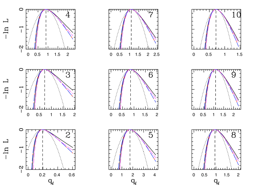
Figure 14: Likelihoods for Phase 2b (12-detector map convolved with an asymmetric beam): Likelihood functions are sampled in each bandpower direction while fixing the other bands at the maximum likelihood values. The black (dotted) curve is the Gaussian approximation given by the Fisher matrix. The blue (dashed) curve is the offset lognormal approximation using the noise $q_{b}^{N}$. The magenta (dash-dotted) curve is the equal variance approximation. The red (dashed) curve is lognormal distribution.The black (solid) curve is the XFaster likelihood estimated for temperature and polarization. The numbers in the right upper corner indicate the multipole $\ell$ or $\ell_{\rm effective}$ of the binned multipoles. As for this set of multipoles $\Delta\ell=1$ these numbers are the single multipole $\ell$

.

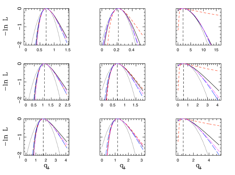
Figure 15: Likelihoods for Phase 2b (12-detector map convolved with an asymmetric beam): Likelihood functions are sampled in each bandpower direction while fixing the other bands at the maximum likelihood values. The black (dotted) curve is the Gaussian approximation given by the Fisher matrix. The blue (dashed) curve is the offset lognormal approximation using the noise $q_{b}^{N}$. The magenta (dash-dotted) curve is the equal variance approximation. The red (dashed) curve is lognormal distribution.The black (solid) curve is the XFaster likelihood estimated for temperature and polarization, for TT (first column), EE (second column) and TE (third column); for $\ell=5$ (first row), $\ell=7$ (second row), $\ell=10$ for TT and TE and for bin with $\ell$ in [10,13] for EE mode (third row).

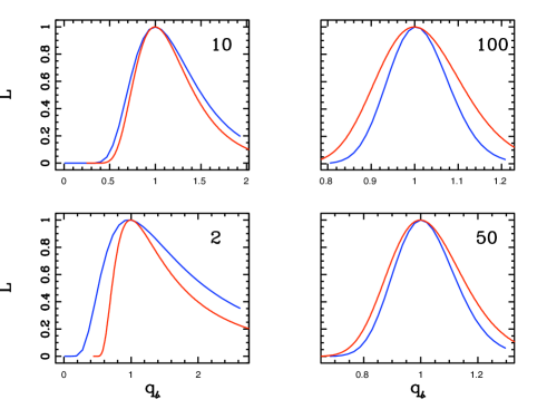
Figure 16: Likelihoods for Phase 2a (12-detector map convolved with a symmetric beam) for TT mode. XFaster likelihood (Phase 2 - cut sky) (blue solid line) vs Exact Full Sky likelihood (Phase 1a - full sky) (red solid line). At low-$\ell$ the XFaster likelihood is wider due to the correlations induced by the cut-sky while at high-$\ell$ XFaster likelihood is narrower due to the binning effect; The numbers in the right upper corner indicate the multipole $\ell$ or the bin number. Up to 10 the bin number is the single multipole $\ell$ as $\Delta\ell=1$, whereas ${\rm bin}=50$ corresponds to $\ell$ in [61,62] and ${\rm bin}=100$ corresponds to $\ell$ in [257,263].

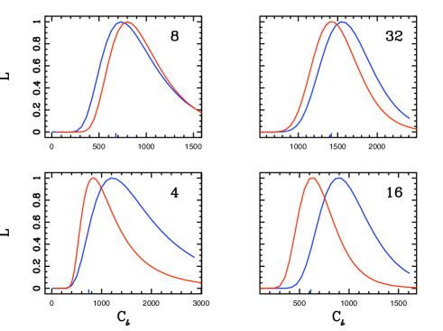
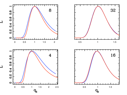
Figure 17: Likelihoods for Phase 2a (12-detector map convolved with a symmetric beam) for TT mode. Left hand side plot: XFaster likelihood slices (blue solid line) versus BFLike, Pixel based likelihood slices (red solid line), both curves are estimated on the cut-sky map of Phase 2. This plot can be misleading as the width of both distributions depend on their peaks locations. Right hand side plot: XFaster likelihood slices (blue solid line) versus BFLike, Pixel based likelihood slices (red solid line), both curves are estimated on the cut-sky map of Phase 2, assuming they both peak at the same value, ie after dividing both distributions by their peaks values. The agreement is already apparent at $\ell$ as low as $\ell=16,32$. The numbers in the right upper corner indicate the multipole $\ell$ or $\ell_{\rm effective}$ of the binned multipoles. As for this set of multipoles $\Delta\ell=1$ these numbers are the single multipole $\ell$

.

4.3 Results: Cosmological parameters

To compare the theoretical power spectrum with the observed power spectrum and estimate parameters, we need an operator to extract theoretical bandpowers from model power spectra $C_{\ell}^{T}$. In Rocha et al. (2010) we considered two types of windows, a top hat window per bin, and the appropriate Fisher-weighted window or XFaster band power window function. These window functions have been used in association with the Offset Lognormal Bandpower likelihood (Rocha et al. (2010)). The XFaster likelihood is estimated multipole by multipole ie for each $\ell$, hence no window function is required. In this mode XFaster can go straight from the map (via its raw pseudo-$C_{\ell}$) to parameter estimation, bypassing the band power spectrum estimation step.

We implemented the XFaster likelihood in a (suitably-modified) version of the publicly-available software CosmoMC (Lewis and Bridle (2002))) for cosmological parameter Markov Chain Monte Carlo estimations. The XFaster likelihood code computes the likelihood of a model passed to it by CosmoMC. There is no need for window functions or the band power spectrum itself. The inputs are the raw pseudo-$C_{\ell}$ of the observations plus the kernel and transfer function required by XFaster to relate the cut-sky pseudo-$C_{\ell}$ to the full-sky $C_{\ell}$.

Figures 18 through 20 show results for a simulation using Phase 2a (symmetric beams) and Phase 2b (asymmetric beams) data. The parameters considered are the baryon, cold dark matter and cosmological constant densities, $\omega_{b}=\Omega_{b}h^{2}$ and $\omega_{c}=\Omega_{c}h^{2}$ and $\omega_{\Lambda}=\Omega_{\Lambda}h^{2}$ respectively, the ratio of the sound horizon to the angular diameter distance at decoupling, $\theta_{s}$, the scalar spectral index $n_{s}$, the overall normalization of the spectrum $\log[10^{10}A]$ at $k=0.05$ Mpc^-1 ($A_{s}$), the optical depth to reionization $\tau$, the age of the universe, the Hubble constant $H_{0}$, and the reionization redshift $z_{re}$.

Figure 19 shows parameters estimated for the average power spectrum of the signal+noise Monte Carlo simulations and for the observed power spectrum (i.e., the power spectrum estimated for the observed map). The parameters for the average simulated data recover the true input parameters, while those for the observed map shift from the input values, particularly for $A_{s}$. As mentioned before, the observed map is a WMAP-constrained realization, i.e., it uses the $a_{lm}$ with phases measured by WMAP up to $\ell=70$ to reproduce the large-scale structure observed by WMAP, and a best-fit model to the WMAP observations for $\ell>70$. The WMAP best-fit parameters are obtained with considerable marginalization of the low-$\ell$ points by foregrounds. They are therefore unaffected by the low-$\ell$ anomalies. This means that unless we do such analysis too, we would not expect our observed realization to agree with the WMAP best fit model. This is clearly shown in Figure 19. On the other hand, as Monte Carlo simulations are realizations of the WMAP best-fit model, one should expect no systematic bias from the ensemble of simulations, as confirmed in Figure 18.

As discussed in section 3, XFaster assumes that the noise is white (uncorrelated), i.e., that the noise covariance matrix is diagonal. Also, the XFaster likelihood is estimated multipole by multipole, hence to estimate the transfer function properly requires a larger number of Monte Carlo simulations to beat down the correlations between multipoles introduced by, e.g., sky cuts required for foreground removal. These simulations include both correlated noise and a sky cut. To assess whether the low-$\ell$ inadequacy of the likelihood is indeed the cause of the parameter offsets seen in Figure 19, we recalculated parameters, this time fixing $\tau$ to the input model value in the simulations. Since $\tau$ and only $\tau$ is constrained almost entirely by the $\ell<30$ data, by fixing $\tau$ we mimic the effect of using a likelihood evaluator that takes full cognizance of correlations in the noise and between multipoles at low $\ell$. The results are shown in Figure 19. The estimated parameters shift towards the input parameter values, recovering those estimated for the average case in agreement with our postulated hypothesis.

Table 1 compares parameter constraints for the symmetric beam case for the ensemble average power spectrum of the Monte Carlo simulations run (avg) and the observed power spectrum run (pse) without $\tau$ fixed. The parameter constraints tabulated are from the marginalised distributions. The parameter constraints for the observed power spectrum run (pse) when $\tau$ is fixed to the fiducial input value are indistinguishable from those derived from the average run, hence very close to the input parameter values. Therefore we do not include them in Table 1.

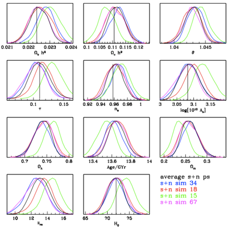
Figure 18: Parameter constraints from Phase 2a (12-detector map convolved with a symmetric beam). The 1-dimensional marginalized posteriors are from XFaster likelihood (with inclusion of all modes, TT, EE, BB, TE): for ensemble average of signal+noise Monte Carlo simulations, i.e., average run (solid black lines), for several single signal+noise Monte Carlo simulations, and for values of the fiducial best fit input parameters (black vertical lines). The parameters for the average power spectrum recover the true input parameters. Furthermore this plot shows that there is no systematic bias for each Monte Carlo simulation. This is to be expected as the Monte Carlo simulations are realizations of the WMAP best fit model.

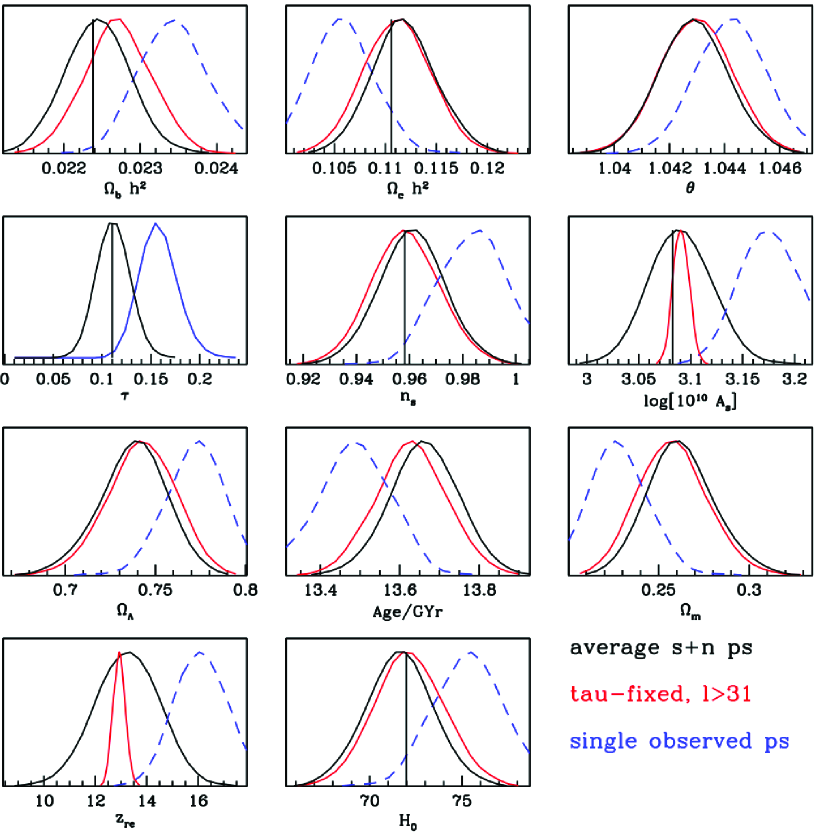
Figure 19: Parameter constraints from Phase 2a (12-detector map convolved with a symmetric beam). The 1-dimensional marginalized posteriors are from XFaster likelihood (with inclusion of all modes, TT, EE, BB, TE): for ensemble average of signal+noise Monte Carlo simulations, i.e., average run (solid black lines), for single observed data (dashed blue lines) and for the run with $\tau=\tau_{fiducial}$ using XFaster likelihood for $\ell>30$ (solid red lines), with overplotted values of the fiducial best fit input parameters (black vertical lines). The parameters for the average power spectrum recover the true input parameters. However the parameters for the observed map shift from the input parameters, particularly so for the parameter Amplitude $A_{s}$. As the large scale structure of the observed map is a WMAP constrained realization we do not expect the estimated parameters to agree with WMAP best fit parameters. Fixing $\tau$ to the input value regularizes the amplitude in the likelihood runs, now the estimated parameters of the observed map shift towards the input parameter values recovering those estimated for the ensemble average of the Monte Carlo simulations.

Figure 20 shows constraints from symmetric and asymmetric beam case for the average power spectrum of the Monte Carlo simulations and the actual observed estimated power spectrum without fixing $\tau$. Most of the parameters for both cases are consistent with each other. Investigating the plot for the average mode, we see deviations of the order of $\sigma/2$ for $\Omega_{c}h^{2}$, $\sigma_{8}$, $n_{s}$ and $H_{0}$. There is an obvious degeneracy between $\sigma_{8}$ and $n_{s}$. For the observed case these deviations are noticeable mostly in $A_{s}$ and $\sigma_{8}$. Once again these parameters are degenerate.

The overall agreement in the parameter constraints from both symmetric and asymmetric beam cases is quite impressive. This reflects the adequacy of our procedure when dealing with beam asymmetries.

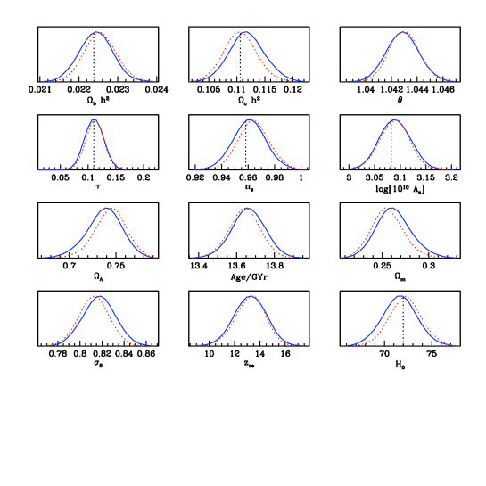
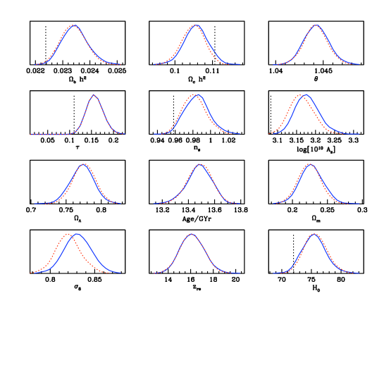
Figure 20: Parameter constraints from Phase 2a (12-detector map). The 1-dimensional marginalized posteriors are from XFaster likelihood (with inclusion of all modes, TT, EE, BB, TE): for the averaged spectra (left hand side) and for single realization spectra (observed map) without fixing $\tau$ (right hand side), asymmetric beam (solid blue lines) and symmetric beam (dashed red lines) cases.

Table 1: Parameter constraints from Planck 70 GHz data, Phase 2a, for map generated with all twelve detectors and convolved with a symmetric beam, using XFaster power spectrum and likelihood estimator for the average of the signal+noise Monte Carlo simulations power spectrum (avg) and the actual observed power spectrum (pse) without $\tau$ fixed. As mentioned in the text, the parameter constraints for the actual power spectrum run (pse) when $\tau$ is fixed to the fiducial input value are indistinguishable from those derived from the average run, hence very close to the input parameter values. Parameter constraints displayed here were obtained from the marginalised distributions.

param	bestfit (avg) $\simeq$ bestfit (pse with fixed $\tau$)	bestfit (pse with varying $\tau$)	input
$\omega_{b}$	$0.0225^{+0.00042}_{-0.00042}$	$0.0231^{+0.00046}_{-0.00046}$	0.02238
$\omega_{c}$	$0.1115^{+0.00309}_{-0.00305}$	$0.1077^{+0.00307}_{-0.00314}$	0.11061
$\theta$	$1.0430^{+0.00120}_{-0.00122}$	$1.0445^{+0.00130}_{-0.00137}$
$\tau$	$0.1105^{+0.00643}_{-0.00771}$	$0.1573^{+0.00833}_{-0.00950}$	0.1103
$n_{s}$	$0.9621^{+0.01130}_{-0.01170}$	$0.9757^{+0.01341}_{-0.01353}$	0.95820
$log[10^{10}A_{s}]$	$3.0874^{+0.02690}_{-0.02748}$	$3.1727^{+0.03270}_{-0.03324}$	3.0824
$\Omega_{\Lambda}$	$0.7394^{+0.01750}_{-0.01843}$	$0.7633^{+0.01710}_{-0.01695}$
$Age$	$13.7^{+0.1}_{-0.1}$	$13.5^{+0.1}_{-0.1}$
$\Omega_{m}$	$0.2606^{+0.01843}_{-0.01749}$	$0.2367^{+0.01698}_{-0.01710}$
$z_{re}$	$13.1^{+1.1}_{-1.1}$	$16.3^{+1.1}_{-1.1}$
$H_{0}$	$71.82^{+1.74}_{-1.81}$	$74.46^{+1.95}_{-1.94}$	71.992

5 Conclusions

The XFaster power spectrum estimator is fully adequate to estimate the power spectrum of Planck data in the high-$\ell$ regime. It also performs well at moderately low multipoles, as long as the low-$\ell$ polarization and temperature power is properly accounted for, e.g., by adding an adequate low-$\ell$ likelihood ingredient. Our minimal non-informative approach enables us to recover most input parameters regardless of the asymmetry of the beam.

Ackowledgments

The work reported in this paper was partially done within the CTP Working Group of the Planck Consortia. Planck is a mission of the European Space Agency. GR would like to say a special thank you to Charles Lawrence for his insightful comments and dedicated help during the writing up of this manuscript. GR is also grateful to Jeff Jewell for useful discussions. This research used resources of the National Energy Research Scientific Computing Center, which is supported by the Office of Science of the U.S. Department of Energy under Contract No. DE-AC03-76SF00098. This work has made use of the HEALPix package (Górski et al. (2005)); and of the Planck satellite simulation package, LevelS, (Reinecke et al. (2005)) which is assembled by the Max Planck Institute for Astrophysics Planck Analysis Centre (MPAC). GR Planck Project is supported by the NASA Science Mission Directorate. The research described in this paper was partially carried out at the Jet propulsion Laboratory, California Institute of Technology, under a contract with NASA. Copyright 2009. All rights reserved.

References

- Ashdown et al. (2007a) Ashdown M. A. J., Baccigalupi C., Balbi A., Bartlett J. G., et al., A&A, 467,761, 2007a
- Ashdown et al. (2007b) Ashdown M., et al., A&A, 471,361, 2007b
- Ashdown et al. (2009) Ashdown M. A. J., Baccigalupi C., Balbi A., Bartlett J. G., et al., A&A, 493,753, 2009
- Ashdown (2009c) Ashdown M. A. J., 2009b, in preparation
- Ashdown et al. (2010) Ashdown M. A. J., Baccigalupi C., Balbi A., Bartlett J. G., et al., 2010, in preparation
- Benabed et al. (2009) Benabed K., Cardoso J.-F., Prunet S., Hivon E., 2009, submitted to MNRAS
- Bond Jaffe & Knox (2000) Bond J. R., Jaffe A. H., Knox L., 2000, ApJ, 533, 19
- Borrill (1999) Borrill J., 1999, in ”Proceedings of the 5th European SGI/Cray MPP Workshop”, Bologna, Italy, arXiv:astro-ph/9911389
- Borrill et al. (2009) Borrill J. et al, 2009, in preparation
- Contaldi et al. (2010) Contaldi C. R., Bond J. R., Crill, Hivon E., et al., 2010, in preparation
- Chon et al. (2003) Chon G., Challinor A., Prunet S., Hivon E., Szapudi I., 2004, MNRAS, 350, 914
- Dupac & Tauber (2005) Dupac,V,& Tauber,J., 2005, A&A, 430, 363
- Efstathiou (2004) Efstathiou G., 2004, MNRAS, 349, 603
- Efstathiou (2005) Efstathiou G., 2005, MNRAS, 370, 343
- Eriksen et al. (2004) Eriksen H. K.,O’Dwyer I. J.,Jewell J. B.,Wandelt B. D., et al., 2004, ApJS, 155, 227
- Górski (1994a) Górski K. M.,1994a, ApJ, 430L, 85G
- Górski et al. (1994b) Górski K. M., et al. 1994b, ApJ. Lett., 430L, 89
- Górski et al. (1996) Górski K. M., et al. 1996, ApJ. Lett., 464L, 11
- Górski (1997) Górski K. M., 1997, Proceedings of the 16th Moriond Astrophysics Meeting: Microwave background anisotropies, p. 77 - 84
- Górski et al. (2005) Górski K. M., Hivon E., Banday A. J., Wandelt B. D., et al., 2005, ApJ, 622, 759-771
- Gruppuso et al (2009) Gruppuso A., De Rosa A., Cabella P., Paci F., accepted for publication in MNRAS
- Hamilton (1997) Hamilton, 1997, MNRAS, 289, 295-304
- Hamimeche & Lewis (2008) Hamimeche S., Lewis A., Phys. Rev. D77, 103013, 2008
- Hancock et al. (1997) Hancock S., Gutierrez C. M, Davies R. D., Lasenby A. N., Rocha G., et al., 1997, MNRAS, 289, 505
- Hivon, Górski et al. (2002) Hivon E., Górski K. M., Netterfield C. B., Crill B. P., et al., 2002, ApJ, 567, 2
- Jewell et al. (2004) Jewell J., Levin, S., & Anderson, C. H. 2004, ApJ, 609, 1
- Knox (1999) Knox, L., 1999, Phys.Rev. D60, 103516
- Lewis and Bridle (2002) Lewis A. and Bridle S., 2002, Phys. Rev. D 66, 103511 [arXiv:astro-ph/0205436].
- Montroy et al (2006) Montroy T. E., Ade P. A. R., Bock J. J., Bond J. R, et al, 2006, ApJ, 647, 813M
- Netterfield et al (2002) Netterfield C. B., Ade P. A. R., Bock J. J., Bond J. R, et al, 2002, ApJ, 571, 604N
- Planck Blue Book (2005) Planck Collaboration, Planck Blue Book, [arXiv:astro-ph/0604069].
- Polenta et al. (2004) Polenta G., Marinucci D., Balbi A., de Bernardis P., et al., CAP 0511 (2005) 001, arXiv:astro-ph/0402428
- Poutanen (2005) Poutanen T., de Gasperis G., Hivon E., Kurki-Suonio H., et al., A&A, 449, 1311, 2006
- Reinecke et al. (2005) Reinecke M., Dolag K., Hell R., Bartelmann M. and Ensslin T., 2005
- Rocha et al. (2010) Rocha G., Contaldi C.R., Colombo L., Bond J.R., Górski K.M., & Lawrence C.R., 2010, in preparation
- Rocha et al. (2010) Rocha G., Contaldi C.R., Bond J.R., Górski K.M., 2010, in preparation
- Smith Challinor & Rocha (2006) Smith S., Challinor A., Rocha G., 2006, Phys. Rev. D37, 023517
- Szapudi et al. (2001) Szapudi I., Prunet S. & Colombi S., 2001, ApJ 548, 115
- Tauber et al (2009) Tauber J., Mandolesi N., Puget J. L., Bersanelli M., et al, Planck Pre-Launch Status: The Planck Mission, 2009, submitted to A&A
- Tegmark, Bunn (1995) Tegmark M., & Bunn E. F., 1995, Ap.J., 455, 1
- Tegmark (1997) Tegmark M., 1997,ApJ, 480, L87-L90
- Tegmark & de Oliveira-Costa (2001) Tegmark M., & de Oliveira-Costa A., 2001, Phys.Rev. D64, 063001
- Tristram et al. (2005a) Tristram M., Macias-Perez J. F., Renault C., Santos D., 2005a, MNRAS, 358, 833
- Tristram et al. (2005b) Tristram M., Patanchon G., Macias-Perez G.F., et al., 2005b, A&A, 436, 785
- Verde et al. (2003) Verde L., Peiris H. V., Spergel D. N., Nolta M. R., et al., 2003, ApJS, 148, 195
- Wandelt, Hivon & Górski (2001) Wandelt B., Hivon E., Górski K. M., 2001, PhR, D64, 083003,
- Wandelt (2001) Wandelt B.D., Górski, K.M., 2001, Phys.Rev. D63, 123002
- Wandelt et al. (2004) Wandelt B. D., Larson, D. L., & Lakshminarayanan, A. 2004, Phys. Rev. D, 70, 083511
- Wright et al. (1994) Wright et al. 1994, ApJ. Lett., 464, L35