Annealing Strategies in the Simulation of Fullerene Formation

Abstract

We investigate the formation of fullerene-like structures from hot Carbon gas using classical molecular dynamics, employing Brenner’s potential. In particular we examine the influence of different annealing strategies on fullerene yield, which is characterized by the distribution of coordination numbers and polygon numbers. It will be shown that the fullerene yield strongly depends on the annealing strategy. Furthermore, we observe a close relation between polygon formation and the number of atoms surrounded by three atoms.

I Introduction

I.1 Fullerenes and Nanotubes

Since their discovery kroto1985 in 1985, fullerenes have been the subject of intense studies, both experimentally and theoretically. These clusters have been identified as roughly spherical carbon “cages”. The fullerene family includes molecules ranging from the (probably unstable) ${\rm C}_{20}$ to fullerenes which contain hundreds or even thousands of carbon atoms. The most stable fullerenes are the soccer ball-like ${\rm C}_{60}$ (also known as buckyball) and the ${\rm C}_{70}$.

All fullerenes have in common the same principal structure: They are composed of $sp^{2}$-hybridized carbon atoms, therefore being closely related to graphite. However, since they are not planar, they can’t be made up entirely of hexagons. The spherical structure is typically achieved by insertion of pentagons. Also Carbon nanotubes Iijima91 , discovered 1991, have a similar structure – the main difference to fullerenes is the enormous aspect ratio (length vs. diameter).

Nanotubes can be interpreted as rolled-up graphite sheets, where the precise procedure of rolling-up decides about the electronic structure of the nanotubes (metallic or semiconducting). So in the absence of defects, nanotubes are composed entirely of hexagons – except the caps which close the tubes.

In the language of classical geometry, fullerenes can be described as polyhedrons, so Euler theorem applies: For an arbitrary polyhedron with $V$ vertices, $E$ edges and $F$ faces, the Euler characteristic $C=V-E+F$ is an invariant, for all simple polyhedrons, $C=2$. From this theorem it can be deduced that any structure which is topologically equivalent to a sphere and only composed of $n_{6}$ hexagons, $n_{5}$ pentagons and $n_{7}$ heptagons must fulfill

$$n_{5}-n_{7}=12$$ (1)

with arbitrary $n_{6}$. So all fullerene molecules will contain exactly 12 pentagons (unless there are heptagons present to compensate for a higher number of pentagons). Therefore, $C_{20}$ is indeed the smallest possible fullerene, composed of 12 pentagons and no hexagons at all.

Since pentagons induce stress, structures which contain adjacent pentagons show reduced stability (isolated pentagon rule, IPR). Obviously, for less then $60$ atoms there is no possibility to avoid this occurrence, and also for $61\leq n\leq 69$ atoms no structure exists which fulfills the IPR. In perfect icosahedral $C_{60}$ two pentagons are always separated from each other by one hexagon, this is the most stable configuration, followed by the rugby-ball like $C_{70}$ which again fulfills the pentagon rule.

Further increasing the number of atoms does not enhance stability. Multiple adjacent hexagons show a graphite-like structure that is more severely disturbed by the pentagons the bigger the molecule gets. So the yield of those fullerenes (for example at arc discharges) is again much smaller than that of $C_{60}$ or $C_{70}$.

I.2 Molecular Dynamics Studies

A natural tool to study the dynamics of fullerene systems is molecular dynamics (MD), where the equations of motion for the nuclei are integrated numericallyRapMD . The most important difference between various types of MD simulations is the way to implement the interaction between the nuclei.

Depending on whether the electronic structure is simulated by ab-initio methodsMarxHutter00 ; Tuckerman02abinitio ; CarParrinello , tight-binding methods TBMDlecture or by more or less elaborate force fields, the accessible system sizes and simulation times vary dramatically.

While there is a wide variety of force-field approaches, certain forms are particularly well-suited for the simulation of (hydro-)carbon systems: Building on the approach of Abell and TersoffAbell85 ; Tersoff86 ; Tersoff88prl ; Tersoff88prb ; Tersoff89 , Donald W. Brenner has developed a potentialBrennerPotential ; Brenner02 for hydrocarbons that is closely related to the potentials obtained in the embedded atom methods (EAM). It contains empirical parameters which were fitted to reproduce the properties of hydrocarbons as well as those of carbon in diamond and graphite.

Its first use was the study of chemical vapor deposition, but found widespread use in various simulations of carbon-based materials. This potential has been incorporated in the BrennerMD codeBrennerMD , which was used for the simulations of sec. II.

MD studies of fullerenes by now encompass a broad range of topics, among others

• studies of nanotube growthTBMDBoronAssist ; GrowthEnergetics ; NanoGrowth95 ; CatGrowth ; XiGrowthDefect ,

• charge structure of nanotube growth from small clustersMelker ,

• nanotube cap formation and energetics StabCapSWCNT ,

• reactive collision of graphite patchesNTNhornGraphPatch which lead to formation of the nuclei of nanotube, nanocage and other structures,

• collisions between fullerenesDefectsCollision ; C60C60Coll and between fullerenes and other moleculesC60CollH2 ,

• the impact of fullerenes on graphite materials C70GraphiteColl ,

• formation of diamond crystallites inside nested carbon fullerenes.DiamNucl

A more comprehensive overview has been given elsewhere DAKL04 . Most interesting in the context of the present article are those studies which deal with formation and fragmentation of fullerenes or fullerene-like structures.

Fullerene stability and fragmentation mechanism have been investigated with a variety of computational methods hussien-2008 , in particular with tight-binding methods. There $\mathrm{C}_{60}$ turned out to be stable against spontaneous disintegration for temperatures up to $5000\;\mathrm{K}$Wang1992 . Similar results have been obtained for other $\mathrm{C}_{n}$-systems.SystStudyStab ; ThermalDisintegration ; Zhang1993b . Most common fragmentation products are dimers, rings and chains; the fragmentation temperature first increases linearly with cluster size, but becomes nearly constant for fullerenes composed of 60 or more atoms.

Other simulationsKim1993 find structural changes in $\mathrm{C}_{60}$ and C₇₀ between $3000$ and $4000\;\mathrm{K}$ and bond breaking around $5000\;\mathrm{K}$. For the melting and evaporation of $C_{20}$, $C_{60}$ and $C_{240}$ one findsMeltingFullerenes a transition from the low-temperature solid to a floppy ”Pretzel phase”, melting at about $T=4000$K and conversion to carbon chain fragments when increasing the temperature to $T\approx 10^{4}$K.

A notable feature of disintegration is the ejection of small clustersTBMDAnnealFrag (in particular $\mathrm{C}_{2}$, sometimes also $\mathrm{C}_{3}$) already below the melting temperature. Similar results for Desintegration and cage formation have been obtained using the TersoffMarcos1999 or BrennerMarayuma1998 potential.

When, studying fullerene formation and using monocyclic, bicyclic, and tricyclic rings as precursorsClassMDFUllForm , the most efficient temperature for the formation of the cage-shaped structure from a ring is about 3000 K. Also the growth process of higher fullerenes through adduction of small carbon clusters and carbon atoms has been studiedContGrowth : In this case small clusters and single atoms easily adsorb on the surface of fullerene cages which have defects, on collisions at thermal velocities; during an annealing process, the attached clusters are soon incorporated into the network of the fullerene cages.

Summarizing these results, most studies find that during the annealing process, one has a sequence of typical steps:

• For very high temperatures, one has a gas of single atoms or dimers.
  

• When cooling down, the dimers tend to form chains that stay short first, but grow to length of $\mathcal{O}(10)$ atoms below $T=7000$K. This phase (“Pretzel phase”MeltingFullerenes ) can be interpreted as liquid-like.
  

• Below $T\approx 5500$K most chains begin to form vaguely spherical structures where most atoms establish an additional bond to reach carbon’s favored coordination number of three. In particular, hexagons, which are sign of locally graphite respectively fullerene-like structures, form.
  

• The precise transition temperature for the change to fullerenes of course depends on the model employed for interaction, but the growth and removal of defects seem to be most efficient around $T=3000\;\mathrm{K}$.
  

The resulting structures are typically graphite- or fullerene-like with lots of defects. The number of defects can be reduced by slow annealing, and it has been possible (e.g. by isolating a fullerene precursor) to obtain perfect fullerene molecules in some simulations.

All these simulations still have a severe drawback, the times accessible by these simulations are still short compared to the timescales relevant for most physical processes relevant for the formation of fullerenes, which is supposed to happen at $\mathcal{O}(s)$. Simulations, however, can reach in the case of rather small systems with severely restricted types of force fields at most $\mathcal{O}(100\,\mathrm{ns})$. In the present paper we address the question, whether this shortcoming can be compensated by the choice of an appropriate annealing strategy.

I.3 Organization of the Paper

The paper is organized as follows: After the introduction to fullerenes (sec. I.1) and corresponding molecular dynamics simulations (sec. I.2), we turn to the basic simulation setup, described in section II.

Our analysis tools are described in section III, where we discuss distribution of coordination number in sec. III.1 and polygon numbers in sec. III.2. In sec. IV we present and discuss our results; in sec. V we summarize them and give a brief outlook.

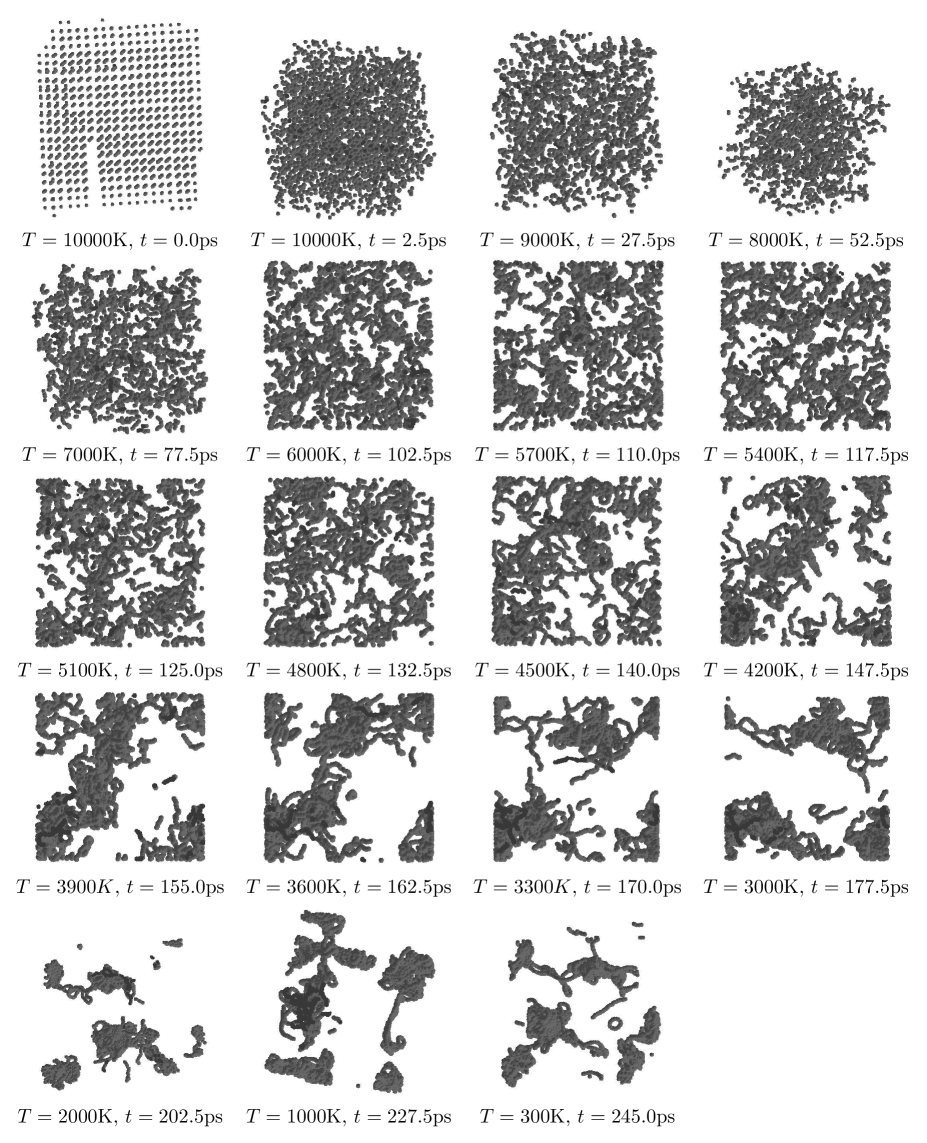
Figure 1: Annealing hot carbon gas: snapshots. This simulation is similar to the ones performed with annealing strategy $T_{1}$, explained in sec. II and illustrated in fig. 3. One can clearly recognize both fullerene-like and chain structures.

II Simulation Setup

Even with modern computing power, the times accessible to MD simulations are still short compared to the timescales relevant for most physical processes to be studied by this method. This also applies to the formation of fullerenes, which is supposed to happen at $\mathcal{O}(\mathrm{s})$ while simulations are typically limited to $\mathcal{O}(100\,\mathrm{ps})$, since one elementary MD step corresponds to $\mathcal{O}(\mathrm{fs})$. At best (studying small systems with cheap and thus severely restricted types of force fields) one can reach $\mathcal{O}(100\,\mathrm{ns})$.

One might expect that this shortcoming can be partially compensated by the choice of an appropriate annealing strategy, e.g. if repeated heating-cooling cycles can significantly improve the fullerene yield – and this is the main question to be studied in this article.

II.1 Examples for Annealing Simulations

We have simulated the annealing of carbon gas from $T\approx 10^{4}$K to room temperature. The simulations have been performed using the BrennerMD codeBrennerMD , which makes use of Langevin dynamics, employing the Fungimol graphical user interfaceFungimol .

An example for such type of simulation is shown in fig. 1 (4024 carbon atoms in a box of $100\,\mathrm{\AA}\times 100\,\mathrm{\AA}\times 100\,\mathrm{\AA}$ with a simulation time of $t=245$ps). The cooling was done in decrements of $100\,\mathrm{K}$ with 5000 thermalization timesteps of $0.5\,\mathrm{fs}$ length in between. So the total simulation lasted $t_{\mathrm{total}}=245\,\mathrm{ps}$ plus a few femtoseconds of initialization steps without thermostat.

The typical stages discussed in sec. I.2 are clearly visible here: the dimer stage, the liquid-like chain phase, the emergence of triple-bound atoms which tend to form planar structures and thus the formation of fullerene-like structures.

Of course many defects occur even in the graphite- or fullerene-like structures; a significant amount of atoms is still contained in long chains even after cooling to room temperature. These chains have (at least for even numbers of atoms) higher ground-state energy than ring-based structures (including graphite, graphene and fullerenes), but they seem to form easier and are favorable at high temperatures due to entropic reasons.

During the annealing process they should convert to smaller rings, but here this is often impossible because of the rapid cooling process. There are some similarities to the formation of an amorphous state via rapid cooling. If – in a very similar setup – the monotonic decrease of temperature is replaced by repeated heating an cooling cycles, the final state typically looks like the one illustrated in fig. 2.

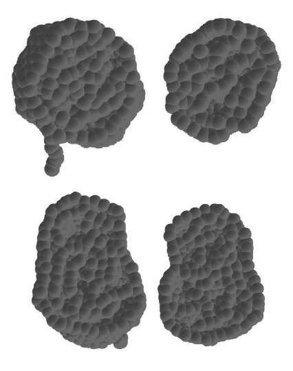
Figure 2: Cut through two final structures obtained by repeated heating and cooling (for two simulations starting with a gas of $N=1620$ atoms)

One still has a considerable amount of long chains, but now they are wound up and enclosed by roughly fullerene-like graphitic cages. The resulting structures can be interpreted as partially frozen droplets with a solid shell, but a liquid core.

II.2 Setup for the Main Simulation

In order to characterize the influence of annealing strategies in a systematic way, we have repeatedly performed several simulations, employing different annealing strategies. In all these simulations the system consists 720 carbon atoms, initially distributed on a simple cubic lattice in a box of $80\,\mathrm{\AA}\times 80\,\mathrm{\AA}\times 80\,\mathrm{\AA}$.

All simulations start with some initialization steps at $T_{\rm initial}=9900\,\mathrm{K}$ and end at the same final temperature $T_{\text{final}}$. In all cases, the total simulation time was $t=300\,\mathrm{ps}$ (600 000 timesteps of $0.5\,\mathrm{fs}$). Data were collected at the beginning of the simulation and every $5\,\mathrm{ps}$ thereafter. Seven different annealing strategies have been employed, which are also depicted in fig. 3:

1. After an initialization period of $24\,000$ steps (corresponding to a simulation time of $12\,\mathrm{ps}$) at $T_{\text{initial}}$K, the temperature is lowered by $\Delta T=100\,\mathrm{K}$ every $6\,000$ timesteps (corresponding to $3\,\mathrm{ps}$) until $T_{\rm final}$ is reached.

2. After the same initialization period as in $T2$, the system is rapidly cooled ($\Delta T=-100\,\mathrm{K}$ every $1\,000$ steps) down to $T=6000\,\mathrm{K}$ at which the system remains for $97\,000$ steps. This process (rapid cooling by $1\,000\,\mathrm{K}$ in $5\,\mathrm{ps}$, followed $48\,\mathrm{ps}$ at constant temperature) is repeated until $T=2000\,\mathrm{K}$ is reached; afterwards rapid cooling is continued down to $T_{\text{final}}$.

3. After the same initialization period as in $T2$, the system is rapidly cooled ($\Delta T=-100\,\mathrm{K}$ every $1\,000$ steps) down to $T=3000\,\mathrm{K}$. After that, the temperature is rapidly ($\Delta T=\pm 100\,\mathrm{K}$ in $0.5\,\mathrm{ps}$) raised to $T=6000\,\mathrm{K}$ and lowered again down to $T=3000\,\mathrm{K}$. This heating-cooling cycle is repeated in total eight times; afterwards the system is further cooled down ($\Delta T=-100\,\mathrm{K}$ in $0.5\,\mathrm{ps}$) to $T_{\text{final}}$.

4. After an initialization period of $56\,000$ steps ($28\,\mathrm{ps}$), the system is rapidly ($\Delta T=-100\,\mathrm{K}$ in $0.5\,\mathrm{ps}$) cooled down to $T=3\,000\,\mathrm{K}$, heated to $T=5\,800\,\mathrm{K}$, cooled to $T=2\,800\,\mathrm{K}$, heated to $T=5\,600\,\mathrm{K}$, cooled to $T=2\,600\,\mathrm{K}$ and so on, until, after heating from $T=1\,600\,\mathrm{K}$ to $T=4\,400\,\mathrm{K}$ the system is cooled down to $T_{\text{final}}$.

5. After an initialization period of $23\,000$ steps, the system is rapidly cooled ($\Delta T=-100\,\mathrm{K}$ every $1\,000$ steps) down to $T=4000\,\mathrm{K}$. After that it is cooled slowly ($\Delta T=-50\,\mathrm{K}$ every $7\,000$ steps) down to $T_{\text{final}}$.

The last two strategies are just variations of $(T3)$, but the heating-cooling cycles operate between $T=2000\,\mathrm{K}$ and $T=5000\,\mathrm{K}$ for (T6) respectively between $T=1000\,\mathrm{K}$ and $T=4000\,\mathrm{K}$ for (T7). The annealing curves for theses seven strategies are displayed in fig. 3.

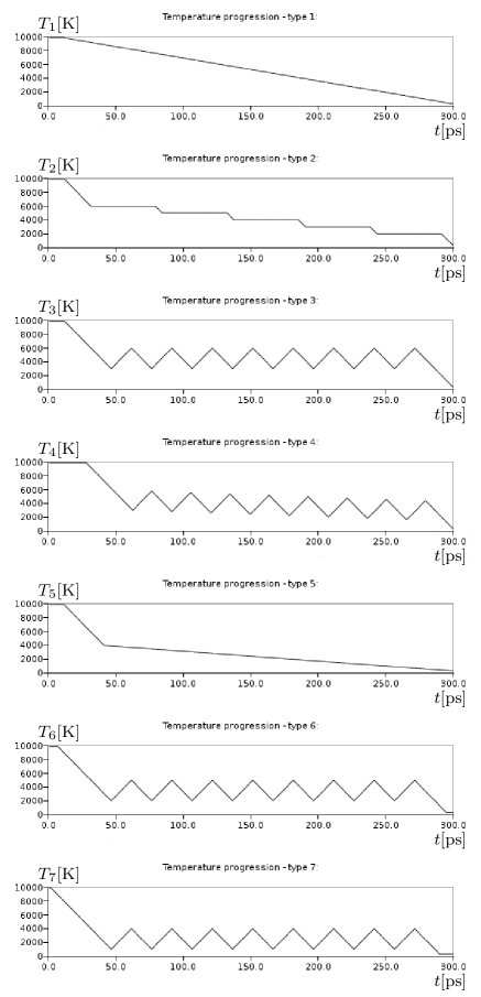
Figure 3: Annealing strategies $T_{1}$ to $T_{7}$ as described in sec. II.2.

III Analysis Tools

In this article we focus on two characteristic quantities: the distribution of coordination numbers and types of polygons present in the system.

III.1 Coordination Numbers

The coordination number $z$ (number of direct neighbors) is characteristic for the phase of carbon. A gas of carbon atoms has $z=0$, for carbon dimers one has $z=1$. Carbon chains and isolated rings have $z=2$. For the $sp^{2}$-hybridized carbon atoms in graphite, graphene, nanotubes and fullerenes one has $z=3$, while diamond structures are characterized by $z=4$.

The bond length of $sp^{2}$-hybridized carbon in graphite layers is $1.42\AA$, for $sp^{3}$-hybridized atoms in diamond one has $1.54\AA$. The carbon-carbon bond lengths in $C_{60}$ are $1.40\AA$ for adjacent hexagons and $1.45\AA$ in pentagons. Similar values one has to expect in other fullerenes or nanotubes. Therefore setting up a threshold of $a^{*}:=1.60\AA$ for the carbon-carbon bond seems to be a reasonable choice. In our simulations, bonds are attached to all pairs of atoms that have a distance smaller than the threshold $a^{*}$. While other values for this threshold have some influence on the results, this effect is small within reasonable limits. We will use a normalized coordination number count

$$q_{z}:=\frac{N_{z}}{N}\;,$$

where $N_{z}$ is the number of atoms with coordination number $z$ and $N$ is the total number of atoms.

III.2 Number of Polygons

Also the number of polygons present in the system is characteristic. Fullerenes are mostly composed of hexagons and several pentagons, whereas pure carbon nanotubes as well as graphite and carbon fibers are made from hexagons only. Heptagons may break the convexity of fullerene structures, they repeatedly appear as defects during cooling processes.

Simulations will be characterized by the normalized number of polygons

$$q_{\alpha} :=\frac{\text{number of polygons of type }\alpha}{N/2}\;.$$

The polygon type can be pentagons ($\alpha=\mathrm{p}$), hexagons ($\alpha=\mathrm{h}$), or heptagons ($\alpha=7$). The number of polygons is normalized to the graphene limit of hexagons, which is $\frac{N}{2}$ if there are $N$ atoms.

In order to determine the number polygons of length $L$, we use a ring number algorithm which is built on a tree-search as depicted in fig. 4.

The idea is as follows. For each atom the algorithm checks whether it is part of a ring of length $L$ ($L=5,\,6,\,7$). The algorithm is repeated for the various values of $L$ and for all atoms. Starting from the initial atom, the list of nearest neighbor (n.n.) atoms is determined. The n.n. list contains those atoms which are not further away from the reference atom than the threshold for the bond length.

In turn, for each atom in the n.n. list the corresponding n.n. list is generated. The procedure is repeated $L$ times. The resulting structure can be regarded as a graph with atoms as nodes and bonds as edges.

So, roughly speaking, for each particle all possible paths of length $L$ starting from the selected atom and leading in each step to one of the nearest neighbors of the current atom, are determined. From all these paths, those for which starting and end point coincide (closed paths) are selected.

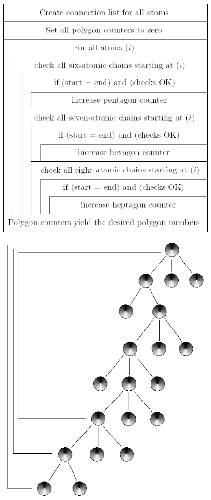
Figure 4: Tree-based polygon search: basic algorithm; graphical representation of six-, seven- and eight-atomic paths

Next we eliminating those structures, in which bonds are repeatedly traversed (as shown in fig. 5a and 5b). When all particles have been checked, the resulting number of detected closed paths of length $L$ equals $2L$ times the number of polygons in the system, since each atom of a polygon is used as initial atom and for each atom there are two possible paths, one clockwise, the other one counter-clockwise.

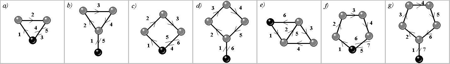
Figure 5: Unwanted polygon findings: (a), (b) false pentagons; (c), (d), (e) false hexagons; (f), (g) false heptagons

IV Results and Discussion

The goal of this paper is to reveal the details of the polygon formation in order to develop an improved annealing strategy. To this end, MD simulations for the different annealing strategies presented above are performed and analyzed. In all simulations, the total number of atoms, initial and final temperatures, as well as the total number of MD steps is the same.

In figs. 6a and 6b the final results are summarized in form of the normalized coordination number count and the normalized number of polygons for the various annealing strategies. An interesting observation of fig. 6b is the fact that the ratio of the number of hexagons to pentagons and heptagons is almost the same in all cases. An exception is strategy $T_{3}$, in which the polygon yield is negligibly small in any case.

A comparison of fig. 6a and 6b reveals that the polygon yield is roughly proportional to the number of atoms with coordination number 3. This implies that polygons are not formed as isolated rings, but rather immediately as locally connected planar structures. The ranking of the annealing strategies in view of the polygon yield is $T_{3}$, $T_{1}$, $T_{2}$, $T_{5}$, $T_{4}$, $T_{7}$, $T_{6}$. The most ineffective strategy of all is clearly $T_{3}$ with almost no polygons, but long chains instead.

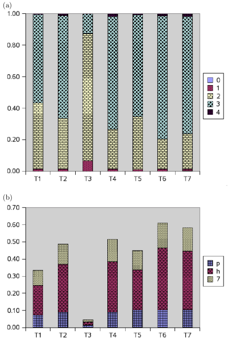
Figure 6: Results: (a) normalized coordination number count $N_{z}$ for $z=(0,1,2,3,4)$ after annealing runs $T_{1}$ to $T_{7}$; (b) number of polygons (pentagons p, hexagons h, heptagons 7), normalized to the graphene limit, for annealing runs $T_{1}$ to $T_{7}$

The expression

$$N_{\rm full}=\frac{\text{number pentagons}-\text{number heptagons}}{12}$$ (2)

could be expected to characterize the number of fullerenes present in a system, provided all carbon atoms are precisely bounded to three other atoms.

In our simulations, however, we find the number of heptagons to be typically larger than the number of pentagons. At second thought, this should not really be surprising since in the “chain phase” the formation of longer rings is more likely than the formation of shorter ones. It shows, however, that we are still quite far from a system which only contains fullerenes.

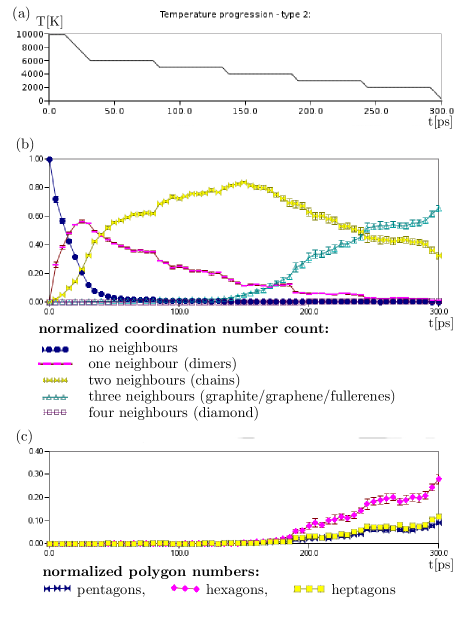
Figure 7: Annealing strategy $T_{2}$: (a) temperature progression; (b) normalized coordination number count; (c) normalized number of polygons.

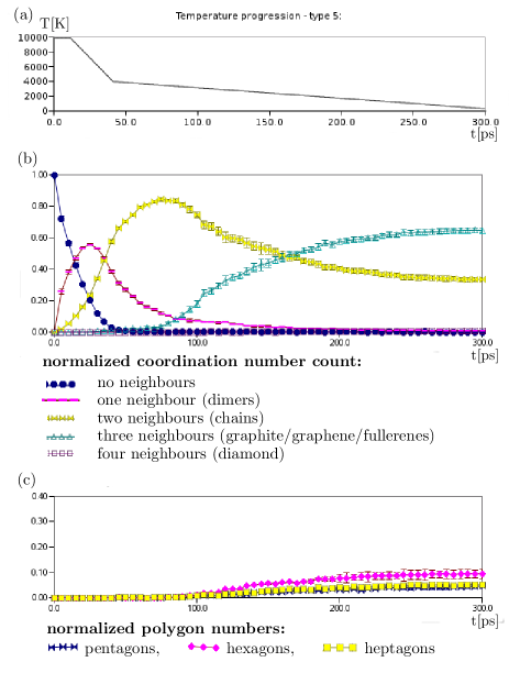
Figure 8: Annealing strategy $T_{5}$: (a) temperature progression; (b) normalized coordination number count, (c) normalized number of polygons.

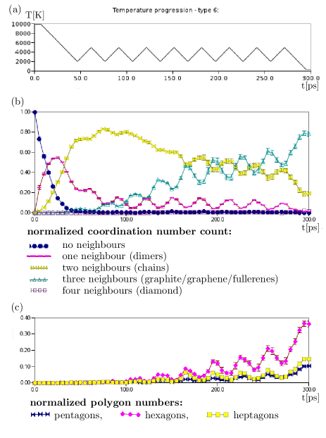
Figure 9: Annealing strategy $T_{6}$: (a) temperature progression; (b) normalized coordination number count, (c) normalized number of polygons.

According to fig. 6 the strategy $T_{3}$ has a very poor polygon yield, while the opposite is true for the best strategy $T_{6}$, although the two annealing strategies look fairly similar. The only but crucial difference is that in the first case the heating-cooling cycles operate between 3000 K and 6000 K, while in second case the temperatures are 2000 K and 5000 K. There are two effects which are expected to be responsible for that:

• In the temperature range of $(2000~{}\mathrm{K},\,3000~{}\mathrm{K})$ lies the crossover temperature $T^{*}_{3}$, at which the number of atoms with coordination number 3 start to dominate over those with coordination number 2. In this range the formation of graphite- or fullerene-like structures seems to be most efficient.

• At the same time the heating-cooling cycles of $T_{6}$ do not exceed (contrary to the $T_{3}$) the onset temperature $T_{o}$ of polygon formation. As we see in fig. 9, the system reacts almost instantaneously on temperature changes, therefore, heating above $T_{o}$ would break up the elementary building blocks of the polygons.

Fig. 7 contains the the detailed time evolution of the normalized coordination count and the normalized number of polygons during the anealing process for strategy $T_{2}$, in which a stepwise cooling is performed with five intermediate temperatures, such that the system is almost in thermodynamic equilibration at the intermediate temperatures. Based on the results in fig 7a we define regions in which atoms of a specific coordination number dominate. We conclude that atoms with coordination number 2 dominate already at $T=10000$ K down to $T=6000$ K. From $T=6000$ K down to a crossover temperature $T^{*}_{3}=2000$ K, atoms with coordination number 2 predominate, while below $T^{*}_{3}$ atoms of coordinations number 3 are in the majority. In the observed temperature range, we found almost no atoms with coordination number 4, the prerequisite for the diamond structure.

The onset of polygon formation, according to fig 7b, takes place at about $t_{p}=90$ ps, while the formation of atoms with coordination number 3 is roughly at $t_{o}=125$ ps. The polygon formation happens right after the cooling from $T=6000$ K to $T=5000$ K, while the formation of atoms with coordination number 3 takes place later at the same temperature. Hence, the polygons are formed first as ringlike structures before they combine locally to form planar structures. Interestingly, the opposite is the case if the system is cooled more rapidly without reaching thermodynamic equilibrium, as is observed in fig. 8.

The onset of polygon formation in fig 8 is at a significant lower temperature than in fig. 7, due to the inertia of the system. Interestingly, the simulation time before polygon formation sets in is the same in both cases. The comparison of coordination number count in both strategies reveals that the system passes through comparable phases, i.e. the depletion of isolated atom, the formation of dimers, the increasing and decreasing number of atoms in chains, followed by the gradual formation of atoms with coordination number 3.

The best of all scrutinized strategies is $T_{6}$, where the systems passes through several heating-cooling cycles. The results are depicted in fig. 9. Although the fraction of atoms with coordination number 3 seems converged in fig. 7a for $T=2000K$ at a value of $q_{z=3}\approx 0.5$, the annealing in $T_{6}$ leads to a significant higher yield of about 0.7 when $T=2000K$ is reached during the last cooling cycle. At the same time the number of atoms with coordination number 2 is reduced by the same amount. Similarly, the number of polygons is roughly increased by $40\%$ in strategy $T_{6}$, when $T=2000$ K is reached during the last cooling cycle.

	8 cycles	16 cycles	24 cycles
$q_{0}$	0	0	0
$q_{1}$	0.013	0.008	0.010
$q_{2}$	0.243	0.178	0.171
$q_{3}$	0.731	0.789	0.796
$q_{4}$	0.013	0.025	0.024
$q_{\text{p}}$	0.119	0.083	0.078
$q_{\text{h}}$	0.358	0.444	0.442
$q_{\text{7}}$	0.152	0.122	0.128

Table 1: Effects of longer simulation runs on the fullerene yield for strategy $T_{6}$. The simulations have been performed for a specific intial configuration and eight, 16, 24 instead of eight)

Exemplary simulations with a strategy similar to $T_{6}$, but a larger number of heating-cooling cycles yield the results given in table 1. The extension from eight to 16 cycles significantly increases the number of triple-bonded atoms (mostly at the expense of double-bonded ones) and the number of hexagons. A further extension to 24 cycles only marginally changes the results, so for this particular strategy we seem to have reached a plateau.

V Summary and Outlook

We have simulated the structures resulting from annealing a hot carbon gas with different strategies, i.e. different forms of temperature evolution. The structures have been analyzed with respect to the coordination number count and the number of pentagons, hexagons and heptagons.

We have found the yield of fullerene-like structures to be quite sensitive to the strategy employed. Thus the fullerene yield can either be significantly enhanced or almost reduced to zero by appropriate annealing strategies.

The best strategy included several heating-cooling cycles, operating below the fullerene disintegration temperature (corresponding to the onset temperature of polygon formation), but encompassing the crossover temperature between double- and triple-bonded atoms

Since timescales in MD simulations are short compared to those of most physical processes, an optimized annealing strategy can be an important means to obtain more realistic results for MD simulations of fullerene formation. Alternatively, repeated heating-cooling cycles which, performed in the optimal temperature window, gave the best fullerene yield, might also occur (on larger timescales) in nature and enhance the fullerene yield e.g. in soot.

While some scrutinized strategies were obviously superior to uniform annealing, it is not at all clear whether we have found an even close-to-optimal strategy in order to maximize the fullerene yield. Here a stochastic optimization (employing simulated annealing or genetic algorithms) of the annealing strategy might provide valuable information on how far the limits can be pushed for short-time simulations.

References

- (1) H. W. Kroto et al., Nature 318, 162, 1985
- (2) S. Iijima, Nature 354, 56 - 58, 1991
- (3) T. Oku, M. Kuno, H. Kitahara, I. Narita, Int. J. of Inorg. Mat. 3, 597-612, 2001
- (4) K. Lichtenegger, Application of Molecular Dynamics Simulation Methods in the Nanoscale Regime, master’s thesis, Graz University of Technology, 2004; available on http://physik.uni-graz.at/kll/nanoMD.pdf
- (5) D. C. Rapaport, The Art of Molecular Dynamics Simulation, Cambridge University Press; Revised Edition, 2004
- (6) F. Ercolessi, A molecular dynamics primer, Trieste, http://www.fisica.uniud.it/ercolessi/md/
- (7) Dominik Marx and Jürg Hutter, NIC Series, Vol. 1, pp. 301-449, 2000, http://www.fz-juelich.de/nic-series/
- (8) Mark E. Tuckerman, J. Phys.: Condens. Matter 14 (2002) R1297-R1355
- (9) R. Car, M. Parrinello, Phys. Rev. Lett., Vol. 55 (1985) 22
- (10) see for example F. Ercolessi, Lecture notes on Tight-Binding Molecular Dynamics, and Tight-Binding justification of classical potentials, available on www.fisica.uniud.it/ercolessi/SA/tb.pdf
- (11) G. C. Abell, Phys. Rev. B 31, 6184 (1985).
- (12) J. Tersoff, Phys. Rev. Lett. 56, 632 (1986).
- (13) J. Tersoff, Phys. Rev. Lett. 61, 2879 (1988).
- (14) J. Tersoff, Phys. Rev. B 37, 6991 (1988).
- (15) J. Tersoff, Phys. Rev. B 39, 5566 (1989).
- (16) D. W. Brenner, Physical Review B 42, 15, 1990
- (17) D. W. Brenner, O. A. Shenderova, J. A. Harrison, S. J. Stuart, and S. B. Sinnott, J. Phys.: Condens. Matter 14, 783 (2002).
- (18) D. Brenner et al., brennermd code, available at http://sourceforge.net/projects/brennermd/
- (19) E. Hernández, P. Ordejón, I. Boustani, A. Rubio and J.A. Alonso, arXiv:cond-mat/0006230
- (20) A. Maiti, C.J. Brabec, C.M. Roland, J. Bernholc, Phys. Rev. Lett. 73 (1994) 18
- (21) A. Maiti, C.J. Brabec, C. Roland, J. Bernholc, Phys. Rev. B 52 (1995) 20
- (22) A. Maiti, C. J. Brabec and J. Bernholc, Phys. Rev. B 55 (1997) 10
- (23) Y. Xia, Y. Ma, Y. Xing, Y. Mu, C. Tan, L. Mei, Phys. Rev. B 15, 61 (2000) 16
- (24) A.I. Melker, S.N. Romanov, D.A. Kornilov, Mater.Phys.Mech.2 (2000) 42-50
- (25) D.-H. Oh, Young Hee Lee, Phys. Rev. B 58 (1998) 11
- (26) T. Kawai, Y. Miyamoto, O. Sugino, Y. Koga, Phys. Rev. B 66, 033404 (2002)
- (27) Y. Xia, Y. Mu, Y. Xing, C. Tan, L. Mei, Phys. Rev. B 56 (1997) 8
- (28) Y. Xia, C. Tan, Y. Mu, Y. Xing, Nucl. Instr. Meth. in Phys. Res. B 135 (1998) 195-200
- (29) Y. Xia, Y. Xing, C. Tan, L. Mei, Phys. Rev. B 52 (1995) 1
- (30) Z. Man, Z. Pan, J. Xie, Y. Ho, Nucl. Instr. Meth. Phys. Res. B 135 (1998) 342-345
- (31) R. Astala, M. Kaukonen, R. M. Nieminen, G. Jungnickel, T. Frauenheim, Phys. Rev.B 63, 081402 (2001)
- (32) A. Hussien, A. Yakubovich, A. Solov’yov, W. Greiner, arXiv.org:0807.4435, 2008
- (33) C. Z. Wang, C. H. Xu, C. T. Chan, and K. M. Ho, J. Phys. Chem. 96, 3563 (1992).
- (34) B.L. Zhang, C.H. Xu, C.Z. Wang, C.T. Chan and K.M. Ho, Phys. Rev. B 46 (1992) 11
- (35) B. L. Zhang, C. Z. Wang, C. T. Chan, and K. M. Ho, Phys. Rev. B 48, 11381 (1993).
- (36) B. L. Zhang, C. Z. Wang, K. M. Ho, and C. T. Chan, Z. Phys. D 26, 285 (1993).
- (37) E. Kim, Y. H. Lee, and J. Y. Lee, Phys. Rev. B 48, 18230 (1993).
- (38) S. G. Kim, D. Tománek, Phys. Rev. Lett. 72, 2418 (1994).
- (39) C. Xu, G. E. Scuseria, Phys. Rev. Lett. 72, 5 (1994) 31
- (40) P. A. Marcos, J. A. Alonso, A. Rubio, and M. J. López, Eur. Phys. J. D 6, 221 (1999).
- (41) Y. Yamaguchi and S. Maruyama, Chem. Phys. Lett. 286, 336 (1998).
- (42) S. Makino, T. Oda, Y. Hiwatari, J.Phys. ChemSolids Vol 58. No. l1.pp. 1845-1851, 1997
- (43) Y. Xia, Y. Mu, Y. Xing, R. Wang, C. Tan, L. Mei, Phys. Rev. B 57 (1998) 23
- (44) T. Freeman, Fungimol, an extensible system for designing atomic-scale objects, available at http://www.fungible.com/fungimol/index.html