Optical response of small closed-shell sodium clusters

Abstract

Absorption spectra of closed-shell Na₂, Na${}_{3}^{+}$, Na₄, Na${}_{5}^{+}$, Na₆, Na${}_{7}^{+}$, and Na₈ clusters are calculated using a recently implemented conserving linear response method. In the framework of a quasiparticle approach, we determine electron-hole correlations in the presence of an external field. The calculated results are in excellent agreement with experimental spectra, and some possible cluster geometries that occur in experiments are analyzed. The position and the broadening of the resonances in the spectra arise from a consistent treatment of the scattering and dephasing contributions in the linear response calculation. Comparison between the experimental and the theoretical results yields information about the cluster geometry, which is not accessible experimentally.

I Introduction

The electronic configuration of small metal clusters is closely connected with their geometrical, chemical and optical properties Knight1 . Different aspects of this interrelation for small metal clusters have been extensively studied experimentally Knight2Exp ; Kappes1Exp ; Kappes2Exp ; Knight3Exp ; deHeer ; Haberland3Exp ; Haberland1Exp ; Haberland2Exp ; Haberland4Exp ; IssendorffExp ; BalettoExp and theoretically ClemengerShell1985 ; BeckJellium1984 ; EckardtJellium1984 ; BrackJellium1993 ; ReinhardJellium2000 ; BortignonExp ; Koutecky31988 ; Koutecky11990 ; Koutecky21990 ; Koutecky41992 ; Koutecky51996 ; RubioPRL1996 ; OgutPRL1999 ; RubioJCP2001 ; UziPRL2001 ; Broglia2005 ; NieminenDFT2008 ; OnidaNa4PRL1995 ; Louie1PRB2000 ; OnidaRMP2002 ; LopezPRB2008 ; Ogut2PRB2009 . For instance, the measured photoabsorption cross section of mass-selected clusters yields important information about the interplay between the underlying nuclear configuration and the electronic structure. However, the geometry of the clusters in the gas phase is not directly accessible in experiments. Ab initio theory can help to determine the structures by choosing, among many possibilities, the most stable geometrical configuration, for which the calculated absorption spectrum is in good agreement with the experimental results.

Early theoretical attempts to understand the nature of electronic correlation in small alkali-metal clusters are based on the shell ClemengerShell1985 and density functional theory (DFT)-based jellium BeckJellium1984 ; EckardtJellium1984 ; BrackJellium1993 ; ReinhardJellium2000 models. Quantum molecular approaches based on the Configuration Interaction (CI) procedures are powerful theoretical tools capable of yielding accurate electronic excited states and important information about the nature of the optically allowed transitions between them. The multi-reference single and double excitation CI has been successfully used to account for the dominant features of the absorption spectra of small sodium clusters Koutecky31988 ; Koutecky11990 ; Koutecky21990 ; Koutecky41992 ; Koutecky51996 , calculated from the oscillator strength of the transitions between the ground and the excited states. Also, time-dependent (TD) DFT methods are widely employed to compute the photoabsorption cross sections of small metal clusters, with various levels of sophistication for the exchange-correlation functional RubioPRL1996 ; OgutPRL1999 ; RubioJCP2001 ; UziPRL2001 ; Broglia2005 ; NieminenDFT2008 . A different way to compute optical spectra is to make use of the quasiparticle picture, where a typical photoabsorption process involves an incoming photon and the transition of an electron from an occupied to an empty quasiparticle state. The determination of the cross section can be achieved by a calculation of a generalized “four-point“ (i.e., two-particle) electron-hole correlation function, which obeys a Bethe-Salpeter equation (BSE) OnidaNa4PRL1995 ; Louie1PRB2000 ; OnidaRMP2002 ; LopezPRB2008 ; Ogut2PRB2009 . In practice, this is usually done in a two-step calculation: first the DFT or Hartree-Fock (HF) single-particle states are used as input into a GW-like procedure to obtain the quasiparticle corrections to the Kohn-Sham or HF ground-state eigenvalues HedinGW ; LouieNaGW . Then a two-particle BS effective equation with a screened direct and an unscreened exchange electron-hole interaction is solved. While the first step properly describes charged excitations (i.e., electron removal or addition, specific to direct or inverse photoelectron experiments), the second step accounts for neutral excitations (i.e., electron-hole pair creation, specific to photoabsorption experiments). A comprehensive comparison between the TDDFT and the GW+BSE approaches can be found in Ref. 32. To facilitate the numerical procedure, the screened Coulomb interaction, which is obtained in the GW step and which enters the BSE, is most often taken to be the statically screened Coulomb interaction. This simplification allows one to cast the effective two-particle BSE in the form of an energy-independent eigenvalue problem, which yields the excited states corresponding to neutral excitations of the system. As in the case of CI, the optical absorption cross section is then determined by the oscillator strengths of the transitions to the excited states, and a phenomenological parameter for the resonance peak broadening is added in order to compare the calculated spectra with the shapes of the experimental peaks. This phenomenological time for the individual transition mimics the combination of thermal broadening and electron lifetime.

We have developed, in a quasiparticle picture, an alternative method to determine the photoabsorption spectra of small sodium clusters. We employ a first-principles based linear response calculation for the dynamical electron-hole correlation function in the presence of an external potential. Although we do assume a ”background” quasiparticle lifetime, the finite width of the absorption peaks contains electron-hole correlation contributions beyond a mere convolution of single-particle lifetimes. A novel aspect of our approach is that we use a quantum kinetic equation for the electron-hole correlations driven by an external coherent optical field to obtain a closed equation for the two-particle BSE without the need of a four-point correlation function. Technically, we include mean-field HF contributions (accounting for direct and exchange bare Coulomb interaction) together with correlation contributions beyond mean-field, described by complicated integral kernels. An important difference from the two-step GW+BSE approaches mentioned above is that we do not include correlations on the single-particle level and then solve the BSE with an effective two-particle interaction described in terms of a simple integral kernel. Instead, we follow the original prescription of deriving conserving approximations for transport equations by Baym and Kadanoff. We thus obtain a BSE for the electron-hole correlation function that is consistent with the electronic single-particle properties BaymKadanoff1961 . This type of conserving approach (in the sense of Baym and Kadanoff) avoids possible problems of double-counting correlation contributions which may arise in a two-step GW+BSE-like calculation due to the separate treatment of single- and two-particle correlations. As already shown by Baym and Kadanoff, such a conserving approach fulfills important sum-rules by construction. For instance, the particle-number conservation law for the electron-hole correlation function, which can be read as a sum rule for the absorption cross section in finite systems, serves as a check of our numerical calculations.

II Theory

The BS approach employed to calculate the absorption spectra is described in detail in Refs. 38 and 39, and is briefly reviewed in the following. The central quantity of this approach is the retarded density-density correlation function $\chi^{\mathrm{r}}(\mathbf{r},t;\mathbf{r^{\prime}},t^{\prime})$, which describes the linear response of the system to an external potential $U(\vec{r},t).$ For finite systems, we use the matrix element

$$\langle n_{1}n_{2}|\chi^{\mathrm{r}}(t,t^{\prime})|n_{3}n_{4}\rangle=\left.\frac{\delta\rho_{n_{2}n_{1}}(t)}{\delta U_{n_{3}n_{4}}(t^{\prime})}\right|_{U=0}$$ (1)

in a basis of HF eigenfunctions $\{\varphi_{n}(\mathbf{r})\}$. Here, $n$ labels the HF spin orbital, and $\rho_{n_{2}n_{1}}(t)=\langle c_{n_{2}}^{{\dagger}}(t)c_{n_{1}}(t)\rangle$ with the annihilation (creation) operators $c_{n}$ ($c_{n}^{{\dagger}}$) for an electron in HF orbital $\varphi_{n}.$ In linear response, the electronic distribution functions $\rho_{nn}$ are unchanged, and the only nonzero elements in Eq. (1) are those with indices that pair occupied and unoccupied states, i.e., Eq. (1) is the electron-hole correlation function.

The photoabsorption cross section is calculated from the Fourier transform of the imaginary part of $\chi^{\mathrm{r}}$ according to

$$\sigma(\omega)=\frac{\omega}{\varepsilon_{0}c}\sum_{n_{1}\dots n_{4}}\mathrm{Im}\langle n_{2}n_{1}|\chi^{\mathrm{r}}(\omega)|n_{3}n_{4}\rangle\,{\mathbf{d}}_{n_{1}n_{2}}\cdot{\mathbf{d}}_{n_{3}n_{4}},$$ (2)

where ${\mathbf{d}}_{n_{1}n_{2}}=\int\varphi_{n_{1}}^{\ast}\,(e\,{\mathbf{r}})\,\varphi_{n_{2}}d^{3}r$ are the electric dipole matrix elements in the molecular orbital representation and $e$ is the electron charge.

The two-particle BS equation for $\chi^{\mathrm{r}}$ is

$$\big{(} \omega-\epsilon_{n_{1}}^{\mathrm{HF}}+\epsilon_{n_{2}}^{\mathrm{HF}}\big{)}\langle n_{1}n_{2}|\chi^{\mathrm{r}}(\omega)|n_{3}n_{4}\rangle+$$

$$(f_{n_{1}}-f_{n_{2}})\Big{[}\delta_{n_{1}n_{3}}\delta_{n_{2}n_{4}}+\sum_{n_{5}n_{6}}\Big{(}\langle n_{1}n_{5}|v|n_{2}n_{6}\rangle$$

$$-\langle n_{1}n_{2}|v|n_{5}n_{6}\rangle\Big{)}\langle n_{5}n_{6}|\chi^{\mathrm{r}}(\omega)|n_{3}n_{4}\rangle\Big{]}$$

$$+\sum_{n_{5}n_{6}}\langle n_{1}n_{2}|\Delta(\omega)|n_{5}n_{6}\rangle\langle n_{5}n_{6}|\chi^{\mathrm{r}}(\omega)|n_{3}n_{4}\rangle=0$$ (3)

with the correlation kernel

$$\langle n_{1}n_{2} |\Delta(\omega)|n_{3}n_{4}\rangle=$$

$$\sum_{n_{5}n_{6}}\Big{[} \frac{f_{n_{1}}(1-f_{n_{5}})f_{n_{6}}+(1-f_{n_{1}})f_{n_{5}}(1-f_{n_{6}})}{\omega-\tilde{\epsilon}^{*}_{n_{6}}+\tilde{\epsilon}_{n_{5}}-\tilde{\epsilon}^{*}_{n_{1}}+\tilde{\epsilon}_{n_{4}}}$$

$$\qquad\times\langle n_{1}n_{5}|v|n_{3}n_{6}\rangle\langle n_{6}n_{2}|v|n_{5}n_{4}\rangle$$

$$+ \frac{f_{n_{2}}(1-f_{n_{5}})f_{n_{6}}+(1-f_{n_{2}})f_{n_{5}}(1-f_{n_{6}})}{\omega+\tilde{\epsilon}_{n_{6}}-\tilde{\epsilon}^{*}_{n_{5}}-\tilde{\epsilon}^{*}_{n_{3}}+\tilde{\epsilon}_{n_{2}}}$$

$$\qquad\times\langle n_{1}n_{5}|v|n_{3}n_{6}\rangle\langle n_{6}n_{2}|v|n_{5}n_{4}\rangle$$

$$-\delta_{n_{1}n_{3}} \sum_{n_{7}}\frac{f_{n_{7}}(1-f_{n_{6}})f_{n_{5}}+(1-f_{n_{7}})f_{n_{6}}(1-f_{n_{5}})}{\omega-\tilde{\epsilon}^{*}_{n_{6}}+\tilde{\epsilon}_{n_{5}}-\tilde{\epsilon}^{*}_{n_{3}}+\tilde{\epsilon}_{n_{7}}}$$

$$\qquad\times\langle n_{4}n_{5}|v|n_{7}n_{6}\rangle\langle n_{6}n_{2}|v|n_{5}n_{7}\rangle$$

$$-\delta_{n_{2}n_{4}} \sum_{n_{7}}\frac{f_{n_{7}}(1-f_{n_{6}})f_{n_{5}}+(1-f_{n_{7}})f_{n_{6}}(1-f_{n_{5}})}{\omega+\tilde{\epsilon}_{n_{6}}-\tilde{\epsilon}^{*}_{n_{5}}-\tilde{\epsilon}^{*}_{n_{7}}+\tilde{\epsilon}_{n_{4}}}$$

$$\qquad\times\langle n_{1}n_{5}|v|n_{7}n_{6}\rangle\langle n_{6}n_{3}|v|n_{5}n_{7}\rangle\Big{]}.$$ (4)

In Eqs. (3) and (II) $f_{n}=\rho_{nn}$ are the level occupation numbers assumed to be equilibrium Fermi-Dirac distributions at $T=0$ K. The bare Coulomb matrix element is defined by

$$\langle n_{1}n_{2}|v|n_{3}n_{4}\rangle =\int d^{3}r_{1}d^{3}r_{2}\,\varphi^{*}_{n_{1}}({\mathbf{r}}_{1})\varphi^{*}_{n_{2}}({\mathbf{r}}_{2})$$

$$\qquad\times\,v(|{\mathbf{r}}_{1}-{\mathbf{r}}_{2}|)\,\varphi_{n_{3}}({\mathbf{r}}_{1})\varphi_{n_{4}}({\mathbf{r}}_{2}).$$

The denominators in the expression for the correlation kernel (II) contain the quasiparticle energies including an inverse lifetime $\tilde{\varepsilon}_{n}=\varepsilon_{n}+i\gamma_{n}$. In principle, one can use for $\tilde{\varepsilon}_{n}$ the results of a quasiparticle calculation such as a GW calculation YaroslavPRL ; PalEPJB ; YaroslavGW , but here we employ the HF energies and a constant broadening for all states whose magnitude is in agreement with GW calculations. We stress that introducing a fixed quasiparticle lifetime for the calculation of $\Delta(\omega)$ does not mean that the broadening of the resonances in $\chi^{\mathrm{r}}$ is given by this value. Rather, the resonance broadening, which is responsible for the finite width of the peaks in the absorption spectrum, is due to the imaginary part of the full correlation contribution $\Delta(\omega)$. The real part of $\Delta(\omega)$ yields the shift in the resonance energies. Both effects, renormalization and broadening of the $\chi^{\mathrm{r}}(\omega)$ spectrum, are thus related.

Equation 3 for the electron-hole correlation can be solved at different levels of approximation. Neglecting all Coulomb interactions and setting

$$\langle n_{1}n_{2}|\Delta(\omega)|n_{3}n_{4}\rangle=i\delta_{n_{1}n_{3}}\delta_{n_{2}n_{4}}\Gamma$$ (6)

one obtains for $\chi^{\mathrm{r}}$ the independent particle (Lindhard) result

$$\langle n_{1}n_{2}|\chi_{0}^{\mathrm{r}}(\omega)|n_{3}n_{4}\rangle=-\frac{\delta_{n_{1}n_{3}}\delta_{n_{2}n_{4}}(f_{n_{1}}-f_{n_{2}})}{\hbar(\omega+i\eta)-\epsilon^{\mathrm{HF}}_{n_{1}}+\epsilon^{\mathrm{HF}}_{n_{2}}}.$$ (7)

Including direct Coulomb matrix elements, exchange elements and correlation contributions in that order, Eq. (3) resembles a BSE in the ladder approximation (denoted by BS-L in the following) plus exchange (BS-LX) and correlation terms (BS-LXC), respectively PalEPJB . Recall that we use loosely here the term BSE for Eq. (3), even though the BSE is usually written for the four-point generalization of $\chi$.

III Photoabsorption spectra of small Na clusters

In this section we discuss photoabsorption spectra of closed-shell Na₂, Na${}_{3}^{+}$, Na₄, Na${}_{5}^{+}$, Na₆, Na${}_{7}^{+}$, and Na₈ clusters. The numerical results are calculated according to Eq. (2) and compared with experiment. We choose clusters with closed-shell configurations with an even number of electrons, for which all molecular orbitals are doubly occupied or empty. Moreover, Na₂, Na${}_{3}^{+}$, and Na₈ are magic-number clusters, for which the number of valence electrons equals the spherical-shell closing-numbers 2 and 8, respectively deHeer . The electron-hole correlation function is determined by solving Eq. (3) with the correlation kernel (II).

To obtain the equilibrium ($T=0$ K) geometrical configuration, we perform a structural optimization using the HF approximation, which yields the single-particle ground state energies and wave functions. For the Na atoms we use the lanl2dz basis set (double-zeta set with relativistic Los Alamos effective core potential) LANL2DZ , in which the $3s^{1}$ valence electron of each Na atom is represented by contracted Gaussian-like atomic orbitals (3s3p/2s2p) while the contribution of the core electrons is treated using effective core potentials (ECP). To test the stability of our results with respect to the basis set used in the calculations, we have also performed calculations with six other basis sets: SHC (Goddard/Smedley ECP) SHC , CEP-4G (minimal set and Stephens/Basch/Krauss ECP), CEP-31G (split valence set) and CEP-121G (triple-split basis set) CEP , LanL2MB (MBS set and Los-Alamos ECP) LANL2DZ , and SDDall (double-zeta set and Stuttgart/Dresden ECP) SDDAll . For larger basis sets such as lanl2dz, SHC, CEP-121G and SDDall the Na-Na distances vary by less than 1% at the end of the geometry optimization, and the peak positions of the absorption spectra differ by less than 0.1 eV. For smaller basis sets the Na-Na distances vary at most by 0.3 Å while the peak positions have deviations of less than 0.3 eV. Overall, a good comparison with experiment is found for lanl2dz, and in the following we refer only to results obtained using this basis set. When the absorption spectra are calculated from the density-density correlation function obtained in the Lindhard, BS-L and BS-LX approximations, we use a constant broadening $\Gamma=0.03$ eV in Eq. (6). When correlation terms $\Delta$ are included in the calculations we use for the quasiparticle inverse lifetime the value $\gamma=0.15$ eV in Eq. (II).

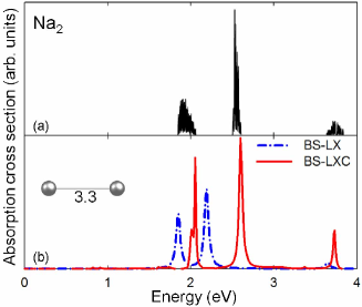
Figure 1: Experimental and calculated absorption spectra of Na₂. (a) Experimental spectrum adapted from Ref. 46. (b) Cross section calculated from $\chi^{\mathrm{r}}$ in the BS-LXC (solid line) and BS-LX (dot-dashed) approximation. The inset shows the cluster structure with the distance in Å.

Within the present approach, the computed spectra should fulfil the $f$-sum rule for finite systems

$$\int{\rm d}\omega\,\omega \sum_{n_{1}\dots n_{4}}\frac{1}{3}\sum_{\mu=x,y,z}d_{\mu,n_{1}n_{2}}d_{\mu,n_{3}n_{4}}$$

$$\times{\rm Im}\langle n_{2}n_{1}|\chi^{\rm r}(\omega)|n_{3}n_{4}\rangle=-\frac{\hbar^{2}\pi}{m}N_{e}$$

for the conserving BS-LX and BS-LXC approximations, Here, $m$ is the electron mass and $N_{e}$ is the total number of electrons in the system. Equation (III) is equivalent to the Thomas-Reiche-Kuhn sum rule for the absorption cross section and is directly related to the particle number conservation law PalEPJB . For our results, Eq. (III) is numerically checked and the $f$-sum rule is fulfilled to better than 99%.

Calculated photoabsorption spectra for Na₂ are shown in Fig. 1 and compared to experimental data. Only when correlations are included in the computation of $\chi^{\mathrm{r}}$, the theoretical spectrum reproduces the experimental absorption peaks which occur around 1.97, 2.55, and 3.75 eV. The pronounced difference between the BS-LX and the BS-LXC results (for the same ground-state cluster geometry which is optimized) shows the importance of electronic correlation contributions to the absorption spectra.

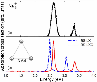
Figure 2: Experimental and calculated absorption spectra of Na${}_{3}^{+}$. (a) Experimental spectrum adapted from Ref. 9. (b) Cross section is calculated in the BS-LXC (solid line) and BS-LX (dot-dashed) approximation. The inset shows the cluster structure with the distances in Å.

In Fig. 2 calculated and experimental results are shown for Na${}_{3}^{+}$. Again, the theoretical spectrum resolves both the larger experimental peak at 2.62 eV as well as the smaller peak at 3.33 eV only when correlations are taken into account. Without correlation contributions, the BS-LX approximation incorrectly describes the positions of the peaks.

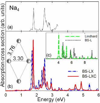
Figure 3: Experimental and calculated absorption spectra of Na₄. (a) Experimental spectrum adapted from Refs. 3 and 4. (b) The cross section obtained from the BS-LXC (solid line) and BS-LX (dot-dashed) approximation. The inset shows the cluster structure with the distances in Å. (c) The spectra obtained from the Lindhard (dashed) and BS-L (dotted) approximations.

In the case of Na₄, the BS-LX and BS-LXC approximations yield peaks in the absorption cross section that are energetically close, as can be seen from the panel (b) of Fig. 3. However, the inclusion of correlation effects results in a better agreement with the experimental spectrum shown in panel (a) of Fig. 3, for which the main peaks are centered around 1.8 and 2.5 eV. Panel (c) shows the calculated spectra corresponding to the Lindhard and the BS-L approximation for $\chi^{\mathrm{r}}$. These approximations yield completely different peak positions that are red shifted with about 2 eV. Moreover, the $f$-sum rule is not fulfilled for the Lindhard and the BS-L approximations, due to the inconsistency between the single- and the two-particle quantities used.

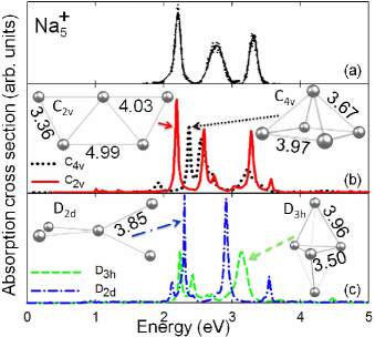
Figure 4: Experimental and calculated absorption spectra of Na${}_{5}^{+}$. (a) Experimental spectrum adapted from Refs. 9 and  10. (b), (c) Cross sections in the BS-LXC approximation for clusters with different symmetries: C_2v (solid line), C_4v (dotted), D_2d (dot-dashed), and D_3h (dashed). The insets show the cluster structures with the distances in Å.

Table 1: Ground-state total energies (in eV) of the Na${}_{5}^{+}$, Na₆, Na${}_{7}^{+}$, and Na₈ clusters for several optimized geometrical structures (shown in the panels (b) and (c) of Figs. 4, 5, 6, and 7, respectively). The configuration with the lowest energy corresponds to the most stable geometry.

Na${}_{5}^{+}$	Na6	Na${}_{7}^{+}$	Na8
-21.605 (D2d)	-29.970 (planar)	-31.866 (D5h)	-40.121 (D${}_{\mathrm{2d}}^{\mathrm{(c)}}$)
-21.476 (C2v)	-29.821 (C5v)	-31.329 (C${}_{\mathrm{2v}}^{\mathrm{(b)}}$)	-39.934 (D4d)
-21.168 (D3h)	-29.526 (D4h)	-30.984 (C3v)	-39.661 (D${}_{\mathrm{2d}}^{\mathrm{(b)}}$)
-20.526 (C4v)	-28.937 (C2v)	-30.829 (C${}_{\mathrm{2v}}^{\mathrm{(c)}}$)	-39.934 (D4d)

To investigate possible geometries of the clusters that may play a role under typical experimental conditions, we consider four different symmetries for Na${}_{5}^{+}$: C_2v, C_4v, D_2d, and D_3h. In Fig. 4 we present spectra calculated in the BS-LXC approximation for each symmetry, and compare them to experiment. As can be seen from the panels (b) and (c) of Fig. 4, the cluster structures which yield the best agreement to the measured cross section correspond to the D_2d and C_2v symmetries. They best resolve the experimental peaks at 2.2, 2.7, and 3.3 eV. The D_2d and C_2v have similar total ground state energies (0.13 eV difference), and are energetically more stable than the D_3h and C_4v structures. In an experiment, at finite temperature, it is possible that both the C_2v and the D_2d clusters are responsible for the shape of the individual peaks, but a clear distinction between the weight of the contribution of each cluster is not possible with a $T=0$ K theory.

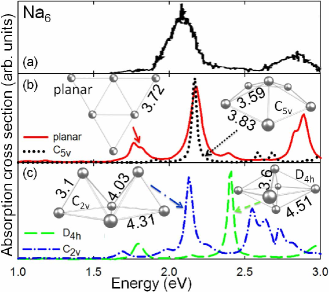
Figure 5: Experimental and calculated absorption spectra of Na₆. (a) Experimental spectrum adapted from Ref. 47. (b), (c) Cross sections in the BS-LXC approximation for clusters with different symmetries: planar (solid line), C_5v (dotted), C_2v (dot-dashed), and D_4h (dashed). The insets show the cluster structures with the distances in Å.

For Na₆ we have also investigated four different symmetries of the cluster structure: planar, C_5v, C_2v, and D_4h. From Fig. 5 one can see that the cross section of the planar and the C_2v geometries agree best with the experimental spectrum. The energetically most stable structure is the planar Na₆. The planar structure overestimates by 0.1 eV the position of the dominant experimental peak at 2.1 eV. It resolves the peak around 2.7 eV, but predicts another peak at 1.75 eV, which is not present in the experimental spectrum. In the case of the C_2v cluster, the most prominent peak agrees well with the experimental peak at 2.1 eV, while the position of the smaller experimental peak around 2.7 eV is underestimated by the calculation by 0.2 eV.

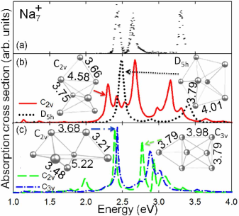
Figure 6: Experimental and calculated absorption spectra of Na${}_{7}^{+}$. (a) Experimental spectrum adapted from Ref. 10. (b), (c) Cross sections in the BS-LXC approximation for clusters with different symmetries: two C_2v (solid and dot-dashed lines), D_5h (dotted), and C_3v (dashed). The insets show the cluster geometries with the distances in Å.

In Fig. 6 we show a comparison between the experimental and the theoretical absorption spectra of Na${}_{7}^{+}$, calculated for two different clusters of C_2v symmetries and also for the D_5h and C_3v geometries. The structure with the most stable energetic configuration is the D_5h, which also reproduces well the 2.4 and 3.3 eV experimental peaks, although with a small offset of 0.1 eV. The experimental peak at 2.4 eV is well reproduced by the structures from panel (c) of Fig. 6, while the C_2v structure from panel (b) resolves well the experimental peak at 2.65 eV.

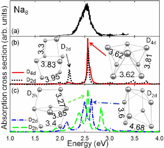
Figure 7: (color online) Experimental and calculated absorption spectra of Na₈. (a) Experimental spectrum adapted from Refs. 3 and 4. (b), (c) Cross sections in the BS-LXC approximation for clusters with different symmetries: D_4d (solid line), two D_2d (dotted and dot-dashed) and D_2h (dashed). The insets show the cluster structures with the distances in Å.

The measured spectrum of the Na₈ cluster in Fig. 7 exhibits a single broad peak extending from 2.2 to 2.8 eV. The theoretical result is computed for four different structural symmetries: D_4d, D_2h, and two different D_2d structures, as shown in Fig. 7. Both the D_4d and the D_2d structures from panel (b) give a pronounced peak around 2.55 eV, which agrees well with the experimental data. However, the D_2d cluster predicts a smaller peak at 2.19 eV not present in the experiment. The D_2d (which has the lowest ground state energy) and the D_2h structures from panel (c) yield several photoabsorption resonance peaks that lie in the same energy interval as the measured spectra. Therefore, different possible configurations of the cluster geometries and finite temperature might be responsible for the strongly broadened experimental line. However, as mentioned above, it is not possible to assign a clear weight for each individual structure computed for $T=0$ K. At finite temperatures phonons are present and the eigenmodes of these vibronic states do not only broaden the peaks, but they may also alter the selection rules, leading to new peaks in the absorption spectra GLyork ; GLPRBphonons .

Summarizing, the calculated BS-LXC spectra presented here are in very good agreement with the measured photoabsorption cross sections, given the potential problems for experiment-theory comparisons which are due to the unknown cluster structures, finite temperature and inhomogeneous broadening effects that tend to wash out the intrinsic spectral features of the resonances.

IV Conclusions

The absorption spectra of small closed-shell Na clusters were calculated by means of a linear response approach for the electron-hole correlation function, defined as the functional derivative with respect to a weak external perturbation of the non-equilibrium single-particle density matrix. We numerically solved a Bethe-Salpeter-like equation for electron-hole correlation that obeys physical conservation laws by construction. In particular, we numerically checked that the $f$-sum rule is fulfilled to better that 99%. We found that correlations effects beyond the mean-field limit need to be included in the calculations in order to properly account for the positions and the widths of the resonance peaks. In the present approach, the finite broadening of the photoabsorption lines is attributed to the correlations between the interacting quasielectrons and holes with a finite lifetime.

The computed cross sections of the clusters displayed an overall good agreement with the measured spectra with respect to the positions and the shapes of the photoabsorption lines. For the smaller clusters Na₂-Na₃ we found the geometrical configurations that yield theoretical spectra in excellent agreement with the experiment. For the larger clusters Na${}_{5}^{+}$-Na₈ we have considered different energetically stable geometries, in order to account, within a $T=0$ K theory, for finite-temperature effects which are unavoidable in experiments. We were able to pinpoint the cluster geometries likely present in the experiments, where the structure cannot be directly obtained.

- (1) W. D. Knight, K. Clemenger, W. A. de Heer, W. A. Saunders, M. Y. Chou, and M. L. Cohen, Phys. Rev. Lett. 52, 2141 (1984)
- (2) W. A. de Heer, K. Selby, V. Kresin, J. Masui, M. Vollmer, A. Chatelain, and W. D. Knight, Phys. Rev. Lett. 59, 1805 (1987)
- (3) C. R. C. Wang, S. Pollack, D. Cameron, and M. M. Kappes, J. Chem. Phys. 93, 3787 (1990)
- (4) C. R. C. Wang, S. Pollack, D. Cameron, and M. M. Kappes, Chem. Phys. Lett. 166, 26 (1990)
- (5) K. Selby, V. Kresin, J. Masui, M. Vollmer, W. A. de Heer, A. Scheidemann, and W. D. Knight, Phys. Rev. B 43, 4565 (1991)
- (6) W. A. de Heer, Rev. Mod. Phys. 65, 611 (1993)
- (7) T. Reiners, W. Orlik, C. Ellert, M. Schmidt, and H. Haberland, Chem. Phys. Lett. 215, 357 (1993)
- (8) C. Ellert, M. Schmidt, C. Schmitt, T. Reiners, and H. Haberland, Phys. Rev. Lett. 75, 1731 (1995)
- (9) M. Schmidt and H. Haberland, Eur. Phys. J. D 6, 109 (1999)
- (10) M. Schmidt, C. Ellert, W. Kronmüller, and H. Haberland, Phys. Rev. B 59, 10970 (1999)
- (11) G. Wrigge, M. Astruc Hoffmann, and B. v. Issendorff, Phys. Rev. A 65, 063201 (2002)
- (12) F. Baletto and R. Ferrando, Rev. Mod. Phys. 77, 371 (2005)
- (13) K. Clemenger, Phys. Rev. B 32, 1359 (1985)
- (14) D. E. Beck, Phys. Rev. B 30, 6935 (1984)
- (15) W. Ekardt, Phys. Rev. Lett. 52, 1925 (1984)
- (16) M. Brack, Rev. Mod. Phys. 65, 677 (1993)
- (17) S. Kümmel, M. Brack, and P.-G. Reinhard, Phys. Rev. B 62, 7602 (2000)
- (18) C. Yannouleas, R. A. Broglia, M. Brack, and P. F. Bortignon, Phys. Rev. Lett. 63, 255
- (19) V. Bonačić-Koutecký, P. Fantucci, and J. Koutecký, Phys. Rev. B 37, 4369 (1988)
- (20) V. Bonačić-Koutecký, P. Fantucci, and J. Koutecký, Chem. Phys. Lett. 166, 32 (1990)
- (21) V. Bonačić-Koutecký, P. Fantucci, and J. Koutecký, J. Chem. Phys. 93, 3802 (1990)
- (22) V. Bonačić-Koutecký, J. Pittner, C. Scheuch, M. F. Guest, and J. Koutecký, J. Chem. Phys. 96, 7938 (1992)
- (23) V. Bonačić-Koutecký, J. Pittner, C. Fuchs, P. Fantucci, M. F. Guest, and J. Koutecký, J. Chem. Phys. 104, 1427 (1996)
- (24) A. Rubio, J. A. Alonso, X. Blase, L. C. Balbás, and S. G. Louie, Phys. Rev. Lett. 77, 247 (1996)
- (25) I. Vasiliev, S. Öğüt, and J. R. Chelikowsky, Phys. Rev. Lett. 82, 1919 (1999)
- (26) M. A. L. Marques, A. Castro, and A. Rubio, J. Chem. Phys. 115, 3006 (2001)
- (27) M. Moseler, H. Häkkinen, and U. Landman, Phys. Rev. Lett. 87, 053401 (2001)
- (28) A. Fortini, M. Mazzola, A. Mina, D. Provasi, G. Colo, G. Onida, H. E. Roman, and R. A. Broglia, J. Phys. B 38, 1581 (2005)
- (29) J.-O. Joswig, L. O. Tunturivuori, and R. M. Nieminen, J. Chem. Phys. 128, 14707 (2008)
- (30) G. Onida, L. Reining, R. W. Godby, R. Del Sole, and W. Andreoni, Phys. Rev. Lett. 75, 818 (1995)
- (31) M. Rohlfing and S. G. Louie, Phys. Rev. B 62, 4927 (2000)
- (32) G. Onida, L. Reining, and A. Rubio, Rev. Mod. Phys. 74, 601 (2002)
- (33) M. L. del Puerto, M. L. Tiago, and J. R. Chelikowsky, Phys. Rev. B 77 (2008)
- (34) M. L. Tiago, J. C. Idrobo, S. Öğüt, J. Jellinek, and J. R. Chelikowsky, Phys. Rev. B 79, 155419 (2009)
- (35) L. Hedin, Phys. Rev. 139, A796 (1965)
- (36) S. Ishii, K. Ohno, Y. Kawazoe, and S. G. Louie, Phys. Rev. B 63, 155104 (2001)
- (37) G. Baym and L. P. Kadanoff, Phys. Rev. 124, 287 (1961)
- (38) G. Pal, Y. Pavlyukh, H. C. Schneider, and W. Hübner, Eur. Phys. J. B 70, 483 (2009)
- (39) G. Pal, Y. Pavlyukh, W. Hübner, and H. C. Schneider, unpublished(2009)
- (40) Y. Pavlyukh, J. Berakdar, and W. Hübner, Phys. Rev. Lett. 100, 116103 (2008)
- (41) Y. Pavlyukh and W. Hübner, Phys. Lett. A 327, 241 (2004)
- (42) P. J. Hay and W. R. Wadt, J. Chem. Phys. 82, 270 (1985)
- (43) A. K. Rappé, T. Smedly, and W. A. Goddard III, J. Phys. Chem. 85, 1662 (1981)
- (44) W. Stevens, H. Basch, and J. Krauss, J. Chem. Phys. 81, 6026 (1984)
- (45) P. Fuentealba, H. Preuss, H. Stoll, and L. v. Szentpaly, Chem. Phys. Lett. 89, 418 (1989)
- (46) W. R. Fredrickson and William W. Watson, Phys. Rev. 30, 429 (1927)
- (47) C. R. C. Wang, S. Pollack, T. A. Dahlseid, G. M. Koretsky, and M. M. Kappes, J. Chem. Phys. 96, 7931 (1992)
- (48) G. Lefkidis, O. Ney, and W. Hübner, phys. stat. solidi (c) 12, 4022 (2005)
- (49) G. Lefkidis and W. Hübner, Phys. Rev. B 74, 155106 (2006)
- (50) N. E. Dahlen and R. van Leeuwen, Phys. Rev. Lett. 98, 153004 (2007)
- (51) K. S. Thygesen and A. Rubio, Phys. Rev. B 77, 115333 (2008)
- (52) J. Rammer and H. Smith, Rev. Mod. Phys. 58, 323 (1986)
- (53) P. Lipavský, V. Špička, and B. Velický, Phys. Rev. B 34, 6933 (1986)
- (54) G. Baym, Phys. Rev. 127, 1391 (1962)
- (55) S. Ismail-Beigi and S. G. Louie, Phys. Rev. Lett. 90, 076401 (2003)
- (56) D. Kremp, M. Schlanges, and W.-D. Kraeft, Quantum Statistics of Nonideal Plasmas (Springer, Berlin Heidelberg New York, 2005)