Modulation of breathers in cigar-shaped Bose-Einstein condensates

Abstract

We present new solutions to the nonautonomous nonlinear Schrödinger equation that may be realized through convenient manipulation of Bose-Einstein condensates. The procedure is based on the modulation of breathers through an analytical study of the one-dimensional Gross-Pitaevskii equation, which is known to offer a good theoretical model to describe quasi-one-dimensional cigar-shaped condensates. Using a specific Ansatz, we transform the nonautonomous nonlinear equation into an autonomous one, which engenders composed states corresponding to solutions localized in space, with an oscillating behavior in time. Numerical simulations confirm stability of the breathers against random perturbation on the input profile of the solutions.

I Introduction

Breathers are solutions of nonlinear equations with a profile which is usually localized in space and periodic in time, even for equations with constant coefficients. Such solutions usually come from a compound of two or more solitons located at the same spatial position. They have been originally introduced in the sine-Gordon equation Ablowitz74 , but they can also be found in other scenarios, controlled by the modified Korteweg-de Vries equation Drazin89 , the Davey-Stewartson Tajiri00 and the nonlinear Schrödinger equation K03 . In various physical systems, which are well described by nonlinear equations, breathers directly affect their electronic, magnetic, optical, vibrational and transport properties, such as in Josephson superconducting junctions 1 ; 2 , charge density wave systems 3 , 4-methyl-pyridine crystals 4 , metallic nanoparticles Meta , conjugated polymers 5 , micromechanical oscillator arrays Micro , antiferromagnetic Heisenberg chains 6 ; 7 , and semiconductor quantum wells Hass09 .

After the first experimental manipulation of Bose-Einstein condensates (BECs) E1 ; E2 ; E3 , studies on bright and dark solitons DS1 ; DS2 ; BS1 ; BS2 have triggered a lot of new investigations, with a diversity of scenarios being proposed and tested K03 ; R1 ; R2 ; B2 ; B3 ; B5 . In particular, the presence of experimental techniques for manipulating the strength of the effective interaction between trapped atoms Rob leads us to believe that in BECs we have an excellent opportunity to investigate breathers of atomic matter waves taking advantage of Feshbach-resonance management ino ; HK ; K3 ; M04 ; PG06 ; H07 ; M05 ; S04 ; Y09 . Thus, in this work the main aim is to show that breathers can be modulated in BECs, presenting a diversity of patterns. We offer an analytical study of such breather solutions of the Gross-Pitaevskii equation (GPE) with both the potential and the parameters that control the strength of the nonlinearities being time-dependent. This makes the GPE nonautonomous and very hard to solve in general. However, we employ an Ansatz which transforms the nonautonomous GPE into an autonomous nonlinear Schrödinger equation (NLSE) which is easier to be studied.

Since the one-dimensional GPE is a very good theoretical model to describe quasi-one-dimensional cigar-shaped BECs B2 ; B3 , we then investigate the presence of the breather behavior in BECs under the assumption that $a_{s}\ll a_{\bot}\ll\lambda\ll a_{||}$, for $a_{s}$ being the scattering length, $\lambda$ the spatial scale of the wave packet, and $a_{\bot}$ and $a_{||}$ being the characteristics transverse and longitudinal trap lengths, respectively. Also, in this work we use potentials and nonlinearities which are typical of BECs, and we believe that the results obtained below may stimulate new experiments in condensates.

In the recent literature, attention has also been devoted to the case of discrete breathers, in arrays of BECs DB1 ; DB2 ; DB3 . However, when one looks for continuous dynamics, with the GPE having variable coefficients depending on the space and time coordinates, analytical solution is not a trivial issue. Here we can point a numerical study M05 which emphasizes the stability properties of the breather excitations in a three-dimensional BEC with Feshbach-resonance management of the scattering length and confined by a one-dimensional optical lattice. We believe that such excitations are made localized by the addition of an external potential, usually created by an optical lattice used to trap them in the lattice.

In the present paper, however, we use a genuine breather solution, i.e., with oscillating behavior in time even when the nonlinear equation presents only constant coefficients (i.e., without modulation). The profile of these breathers are shown in Fig. 1. We also show that they can be modulated in space and time, controlled by the trapping potential and the strength of the cubic nonlinearity, as we show below for a diversity of situations. The procedure is similar to the former investigations SH ; SH2 ; SHB ; BB ; BBC ; ABC , but here we allow for the autonomous NLSE to be partial differential equation, and this introduces an interesting difference which we explore below.

We start the investigation in the next section, where we present the general formalism, following as close as possible the two recent works BB ; ABC . In Sec. III we illustrate the formalism with distinct examples, identified by the trapping potential and cubic nonlinearity, with a diversity of solutions. We also show in Sec. IV, through numerical simulation, that the solutions found in Sec. III are all stable under random perturbation of 5% in their input profile. There we also comment of the case of nonpolynomial nonlinearity, which can be used to compensate for the one-dimensional approximation of real condensates. There we show that the one-dimensional approximation used in this work is reliable. We finish the work in Sec. V, where we introduce the ending comments.

II Formalism

We start with the one-dimensional GPE with the general form

$$i\psi_{t}=-\frac{1}{2}\psi_{xx}+V(x,t)\psi+P(|\psi|^{2})\psi,$$ (1)

where $V(x,t)$ is the potential and $P(|\psi|^{2})$ is given by

$$P(|\psi|^{2})=\sum_{n=1}^{N}g_{2n+1}(t)|\psi|^{2n}.$$ (2)

The coefficients $g_{2n+1}(t)$ of the polynomial function above describe the strength of the nonlinearities present in the system. Here we are using standard notation, in which $x$, $t$ and all other quantities are dimensionless.

Our goal is to find breather solutions of the Eq.(1). Using the Ansatz

$$\psi(x,t)=\rho(t)e^{i\eta(x,t)}\Phi(\zeta(x,t),\tau(t)),$$ (3)

we can change the nonautonomous GPE for an autonomous NLSE that may engender the breather solutions; it is given by

$$i\Phi_{\tau}=-\frac{1}{2}\Phi_{\zeta\zeta}+Q(|\Phi|^{2})\Phi,$$ (4)

where $Q(|\Phi|^{2})$ has the form

$$Q(|\Phi|^{2})=\sum_{n=1}^{N}G_{2n+1}|\Phi|^{2n}.$$ (5)

The coefficients $G_{2n+1}$ are now constant parameters. Using (3) in (1) leads to (4), for $\rho$, $\eta$, $\zeta$ and $\tau$ obeying the following equations

$$\tau_{t}=\zeta_{x}^{2},$$ (6a)

$$\eta_{x}=-\frac{\zeta_{t}}{\zeta_{x}},$$ (6b)

$$\rho_{t}+\frac{\rho\eta_{xx}}{2}=0.$$ (6c)

Here the potential and nonlinearities assume the form

$$V(x,t)=-\eta_{t}-\eta_{x}^{2},$$ (7)

and

$$g_{2i+1}(t)=\frac{G_{2i+1}\zeta_{x}^{2}}{\rho^{2i}},\;\;\;\;i=1,2,3,...$$ (8)

We introduce $a(t)=\sqrt{\tau_{t}}$ to get from (6a) the relation $\zeta=a(t)x+b(t)$. This is important because through $\zeta$ we can now determine the width of the localized solution in the form $1/a(t)$ and its center-of-mass position as $-b(t)/a(t)$; see, e.g., Ref. BB . In the same way, through the use of (6b) one can write

$$\eta(x,t)=-\frac{a_{t}}{2a}x^{2}-\frac{b_{t}}{a}x+c(t).$$ (9)

Thus, using (9) in (6c) one gets $\rho=\sqrt{a}$. Next, we rewrite the potential in the form

$$V(x,t)=f_{1}(t)x^{2}+f_{2}(t)x+f_{3}(t),$$ (10)

with

$$f_{1}(t)=\frac{a_{tt}}{2a}-\frac{a_{t}^{2}}{a^{2}},$$ (11a)

$$f_{2}(t)=\frac{b_{tt}}{a}-\frac{2a_{t}b_{t}}{a^{2}},$$ (11b)

$$f_{3}(t)=-c_{t}-\frac{b_{t}^{2}}{2a^{2}}.$$ (11c)

In this case, $g_{2i+1}(t)=G_{2i+1}a^{2-i}$, for $i=1,2,3,...$, and the nonlinearities assume a simple form. However, we note that in the above general procedure one needs that $g_{5}=G_{5}$, suggesting that the strength of the quintic nonlinearity of the GPE (1) has to be constant.

Similar ideas have been used recently in Refs. SH ; SH2 ; SHB ; BB ; BBC ; ABC . There one changes the nonautonomous NLSE to an autonomous NLSE depending on a single coordinate, in the form of a static-like ordinary differential equation supporting soliton solutions. Such soliton solutions can be modulated via spatial and temporal dependences associated with the potential and nonlinearity present in the nonautonomous NLSE. In this way, the soliton can be modulated in a time-oscillating pattern, as a breather solution; see, e.g., Ref BB for a recent investigation. In our procedure, however, we maintain the nonlinear equation in the form given by Eq. (4), which is a partial differential equation which possesses breather solution even in the absence of the spatial and temporal modulations of the potential and cubic nonlinearity. This introduces an interesting difference because now we are directly controlling the breather solutions. We explore this possibility in the next section, investigating several distinct models.

III Specific models

Let us now turn attention to the case of cubic nonlinearity, with the strength $g_{3}(t)=g(t)$ and no other nonlinearity, which occurs for BECs with strong two-body scattering such as Rb or Na by use of Feshbach-resonance. In this case, the integrability of the NLSE (4) for cubic nonlinearity allows that one obtains breather solutions with distinct profile. A specific form of the two-soliton breather solution is obtained for $G_{3}=G=-1$, which corresponds to the explicit solution SatsumaPTPS74

$$\Phi(\zeta,\tau)=\frac{4(\cosh(3\zeta)+3e^{4i\tau}\cosh(\zeta))e^{i\tau/2}}{(\cosh(4\zeta)+4\cosh(2\zeta)+3\cos(4\tau))}.$$ (12)

It presents the simple form $\Phi(\zeta,0)=2\,{\rm sech}(\zeta)$ at $\tau=0$. This is the simplest case, which we use to investigate distinct models below.

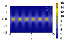
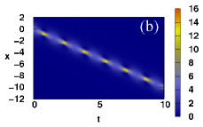
Figure 1: (Color online) Breather solutions of the GPE (1), in the case of a vanishing potential and constant cubic strength. In (a) we display the case $a\!=\!1$ and $b\!=\!0$ and in (b) $a\!=\!1$ and $b\!=\!t$, making the breather to move in space.

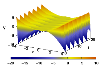
Figure 2: (Color online) Plot of the potential shown in (13), using the parameters $a=1/(1+\cos^{2}(t))$ and $b=0$.

III.1 Vanishing potential

Firstly, we study the free evolution with vanishing potential and constant cubic nonlinearity strength. This case gives the standard breather solution, with the NLSE with zero potential and constant coefficients. Thus, we consider $a=1$, which corresponds to $g=-1$ and $f_{1}=0$, and we take $c_{t}=-b_{t}^{2}/2a^{2}$, leading to $f_{3}=0$. We can make $f_{2}=0$ for $b=0$ and for $b=t$. These breathers are standard solutions and they are plotted in Figs. 1a and 1b, respectively. We note from (1) that for $b=0$, the breather is localized in space and oscillates in time; however, for $b=t$ the corresponding center of mass moves in space with oscillating time behavior. This behavior is related to Eq. (3), and to the nonzero phase in Eq. (9), together with the fact that here $\rho$ is a constant and the form of the solution $\Phi$ in Eq. (12) also contributes with a nontrivial phase: the overall effect is that $b=t$ makes the condensate to move away from its starting position, as it is explicitly shown in Fig. 1b. The oscillation period and frequency of the breather is of approximately $1.57$ and $0.64$, respectively. We obtain the limits for minimum and maximum amplitude equal to $4$ and $16$, respectively, and the time width at half height is approximately $0.39$. Recall that we are using dimensionless coordinates.

III.2 Flying bird potential

Next, we deal with the specific case of a potential with space and time dependence, and a cubic nonlinearity with time-dependent strength. Here we choose the nonlinearity in the form $g=-1/(1+\cos^{2}(t))$. To get a simple potential we take $b=0$ and $c=0$, which make $f_{2}=0$ and $f_{3}=0$. In this case we get to the potential

$$V=\frac{2\cos(2t)}{3+\cos(2t)}\,x^{2}.$$ (13)

Figs. 2 and 3 show the potential and the breather solution, $\left|\psi\right|^{2}$, respectively. This potential changes from attractive to expulsive behavior controlled periodically Exp1 ; Exp2 ; Exp3 . We call this the flying bird potential, since it simulates the wings of a flying bird. Here we note that, differently from the first case, the periodic modulation does affect the periodic behavior of the breather solution. This interesting behavior appears from Figs. 1 and 3: there one sees that the breather exhibits a reduction in its oscillation frequency, which is modulated through the trapping potential and the strength of the cubic nonlinearity.

We see that the oscillation period and frequency of the breather is of approximately $3.14$ and $0.32$, respectively. Note that the breather frequency was reduced by half when compared with the former case. Also, we obtain the limits for minimum and maximum amplitude equal to $2$ and $16$, respectively, and the time width at half height is approximately $0.54$.

The procedure can induce another important behavior to the solution. We can make the breather to move with the choice of $b$ such that $b=-\tan(t)/16(\tan^{2}(t)+2)+3\sqrt{2}\arctan(\tan(t)/\sqrt{2})/32$, to get $f_{2}=0$; also, the choice $c_{t}=-b_{t}^{2}/2a^{2}$ makes $f_{3}=0$. In this way, using the same nonlinearity above the potential is also the same shown in (13). But now the breather present a nontrivial phase in (9), and it presents an interesting behavior: it seems to split in two parts in the time coordinate. This is different from the spatial splitting which was studied before in S04 ; Y09 . Our solution is depicted in Fig. 4, and the breather seems to have two distinct time scales.

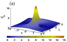
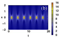
Figure 3: (Color online) Plots of the (a) breather solution and (b) its profile, for the potential depicted in Fig. 2.

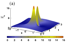
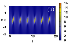
Figure 4: (Color online) Plots of the (a) breather solution and (b) its profile. Here we are using $a$ and $b$ as in Fig. 2.

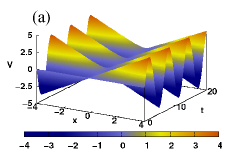
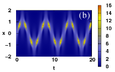
Figure 5: (Color online) Plots of the (a) potential shown in (14) and (b) the corresponding moving breather solution for $a$ constant and $b=\sin(t)$.

III.3 Seesaw potential

Another example is to verify the behavior of the moving breather solution in presence of a potential with linear spatial dependence. To this end we choose $f_{1}=0$, through the use of constant nonlinearity $a=1$, with $f_{3}=0$ for $c_{t}=-b_{t}^{2}/2a^{2}$. Thus, $b=-\sin(t)$ corresponds to the potential

$$V=\sin(t)\,x.$$ (14)

This potential has a seesaw behavior, as it is displayed in Fig. 5a. In Fig. 5b we show the zig-zag pattern of the corresponding breather solution. In this case, the period of oscillation and frequency of the breather solution are $1.57$ and $0.64$, respectively; note that these values are the same of the first case. The amplitude now oscillates between $4$ and $16$ and the time width at half height is approximately $0.41$.

III.4 Another potential

Other potentials can be studied for different values of $a$ and $b$. For instance, using the cubic nonlinearity strength $g=-1/(1+\cos^{2}(t)),$ with $b=t$, and making $f_{3}=0$ we obtain the following potential

$$V\!=\!\frac{2\cos(2t)}{3+\cos(2t)}\,x^{2}-[1+5\cos^{2}(t)]\sin(t)\,x.$$ (15)

It is displayed in Fig. 6. In this case, the breather solution presents an interesting moving pattern, as shown in Fig. 7a, for $b=\sin(t)$. Also, in Fig. 7b we display the behavior of the moving breather considering $b=\sin(\sqrt{2}t)$. With these choices, the breather can present periodic or quasiperiodic pattern, respectively, as it appears explicitly in the Figs. 7a and 7b. In the case of periodic pattern, we obtain the oscillation period of $3.14$ and frequency of $0.32$, with the time width at half height given by $0.56$.

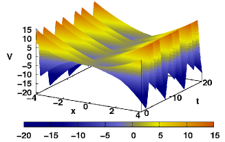
Figure 6: (Color online) Plot of the potential shown in (15).

Figure 7: (Color online) Plots of the profile of the moving breather solution, showing the case of (a) periodic [$b=\sin(t)$] and (b) quasiperiodic [$b=\sin(\sqrt{2}t)$] patterns.

IV Numerical simulations

Starting with the GPE (1) in the case of cubic nonlinearity, we employ a numerical study focusing on the propagation of the modulated breather solution in the form given by Eq. (3). The numerical method is based on the split-step finite difference algorithm with a Crank-Nicolson method to solve the dispersive term in (1). It is known that the Crank-Nicolson method is unconditionally stable Vesely94 . In this way, using a short length of time one can obtain the true pulse propagation. Here, we used the time and space step-size of $0.0001$ and $0.01$, respectively. Thus, with a random perturbation of $5\%$ in the input profile the solution can expose its stable or unstable behavior. All the solutions were tested and appeared to be stable under the suggested random perturbations. We analyzed the solutions for a very long time, until the rescaled time $t=10000$. The results strongly suggest experimental verification of the above breather excitations in condensates.

Another important question to be considered is related to the validity of the one-dimensional approximation to BECs, which we are using in this work. Evidently, we are assuming the regime $a_{s}\ll a_{\bot}\ll\lambda\ll a_{||}$, where the Eq. (1) is supposed to be valid. However, a more general possibility appears when one thinks of considering the quasi-one-dimensional dynamics, which can be treated through a nonpolynomial nonlinear equation, as shown, for instance, in the recent works NP1 ; NP2 ; NP3 ; NP4 ; NP5 . In this case, the Ansatz used in Eq. (3) does not transform the nonautonomous equation into an autonomous one.

To get further information on this issue, let us compare the results obtained in the present study with a numerical investigation of the quasi-one-dimensional equation in presence of nonpolynomial nonlinearity given by NP1 ; NP2 ; NP3 ; NP4 ; NP5

$$i\psi_{t}=-\frac{1}{2}\psi_{xx}+V(x,t)\psi+\frac{1+(3/2)g(x,t)|\psi|^{2}}{\sqrt{1+g(x,t)|\psi|^{2}}}\psi.$$ (16)

Note that for a weak-coupling regime, i.e., $g(x,t)|\psi|^{2}\ll 1$, one can easily obtain the effective one-dimensional Eq. (1); see e.g., NP4 for more details on this issue. In our model, this weak-coupling regime is contemplated when one decreases $a(t)$, i.e., when one increases the width of the localized solution. As a simple example, let us compare the case A of a vanishing potential, studied above, with that obtained numerically through Eq. (16). We use the solution (12) at $t=0$ as initial input in (16) with $a=0.1$ and $b=0$, which correspond to $g=-0.1$ and $V=0$. The results are shown in Fig. 8. Note that the solid (blue) curve presents a slight delay, compared to the dashed (orange) curve which represents case A, of vanishing potential. We believe that this delay is due to the ${\rm max}\,(g|\psi|^{2})\simeq 0.16$, which should be interpreted as $\ll 1$. The results depicted in Fig. 8 in solid (blue) line and in dashed (orange) line reinforces the present study, showing that the one-dimensional approximation used in this work is reliable.

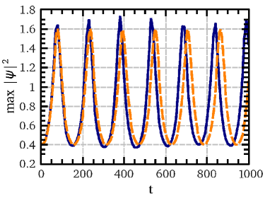
Figure 8: (Color online) Plots of max $|\psi|^{2}$ for comparison between the cubic (orange, dashed line) and nonpolynomial (blue, solid line) nonlinearities, considering $g=-0.1$ and $V=0$.

V Ending comments

In summary, we have studied the modulation of breather excitations in a nonautonomous GPE. We have used an Ansatz to transform the GEP into an autonomous NLSE which supports breathers. The procedure allowed us to investigate a diversity of solutions, each one with its distinctive behavior. The standard breather behavior appears in the simple case, with vanishing potential and constant nonlinearity strength. But we could find other features, such as the moving, and the periodic or quasiperiodic behavior.

We have studied stability numerically, with the results showing that all the breather excitations which we have found are stable against random perturbation on the input profile of the solutions. Also, we have investigated a simple case of nonpolynomial potential, and the results show that the one-dimensional approximation which we have used in the work is reliable. The present study opens several new possibilities, in particular on the experimental search for breather excitations in cigar-shaped condensates, and on extensions of the procedure to condensates with more general nonlinearities and in higher dimensions.

References

- (1) M. J. Ablowitz et al., Stud. Appl. Math. 53, 249 (1974).
- (2) P. G. Drazin and R. S. Johnson, Solitons: an Introduction (Cambridge University Press, 1989).
- (3) M. Tajiri and T. Arai, Proc. Inst. Math. Natl. Acad. Sci. Ukr 30, 210 (2000).
- (4) Y. S. Kivshar and G. P. Agrawal, Optical Solitons: From Fibers to Photonic Crystals (Academic Press, San Diego, California, USA, 2003).
- (5) E. Tr as, J. J. Mazo, and T. P. Orlando, Phys. Rev. Lett. 84, 741 (2000).
- (6) P. Binder et al., Phys. Rev. Lett. 84, 745 (2000).
- (7) H. Kleinert and K. Maki, Phys. Rev. B 19, 6238 (1979).
- (8) F. Fillaux, C. J. Carlile, and G. J. Kearley, Phys. Rev. B 58, 11416 (1998).
- (9) H. Portales et al., J. Chem. Phys. 115, 3444 (2001).
- (10) S. Adachi, V. M. Kobryanskii, and T. Kobayashi, Phys. Rev. Lett. 89, 027401 (2002).
- (11) M. Sato et al., Phys. Rev. Lett. 90, 044102 (2003).
- (12) R. Morisaki et al., J. Phys. Soc. Jpn. 76, 063706 (2007).
- (13) E. Orignac et al., Phys. Rev. B 76, 144422 (2007).
- (14) F. Hass et al., Phys. Rev. 80, 073301 (2009).
- (15) M. H. Anderson et al., Science 269, 198 (1995).
- (16) C. C. Bradley et al., Phys. Rev. Lett. 75, 1687 (1995).
- (17) K. B. Davis et al., Phys. Rev. Lett. 75, 3969 (1995).
- (18) S. Burger et al., Phys. Rev. Lett. 83, 5198 (1999).
- (19) J. Denschlag et al., Science 287, 97 (2000).
- (20) K. E. Strecker et al, Nature 417, 150 (2002).
- (21) L. Khaykovich et al. Science 296, 1290 (2002).
- (22) F. Dalfovo et al., Rev. Mod. Phys. 71, 463 (1999).
- (23) A. J. Legett, Rev. Mod. Phys. 73, 307 (2001).
- (24) C. J. Pethick and H. Smith, Bose-Einstein condensation in dilute gases (Cambridge University Press, Cambridge, UK, 2002).
- (25) L. P. Pitaevski and S. Stringari, Bose-Einstein condensation (Oxford University Press, Oxford, UK, 2003).
- (26) B. A. Malomed, Soliton management in periodic systems (Springer, New York, 2006).
- (27) J. L. Roberts et al., Phys. Rev. Lett. 86, 4211 (2001).
- (28) S. Inouye, Nature 392, 151 (1998).
- (29) E. Timmermans et al., Phys. Rep. 315, 199 (1999).
- (30) P.G. Kevrekidis et al., Phys. Lett. 90, 230401 (2003).
- (31) G. D. Montesinos, V. M. Pérez-García, P. J. Torres, Physica D 191, 193 (2004).
- (32) V. M. Pérez-García, P. J. Torres, V. V. Konotop, Physica D 221, 31 (2006).
- (33) G. Herring et al., Phys. Lett. A 367, 140 (2007).
- (34) M. Matuszewski et al., Phys. Rev. Lett. 95, 050403 (2005).
- (35) H. Sakaguchi and B. A. Malomed, Phys. Rev. E 70, 066613 (2004).
- (36) H. Yanay, L. Khaykovich, and B. A. Malomed, CHAOS 19, 033145 (2009).
- (37) A. Trombettoni and A. Smerzi, Phys. Rev. Lett. 86, 2353 (2001).
- (38) O. Morsch and M. Oberthaler, Rev. Mod. Phys. 78, 179 (2006).
- (39) S. Flach and A. V. Gorbach, Phys. Rep. 467, 1 (2008).
- (40) V. N. Serkin and A. Hasegawa, Phys. Rev. Lett. 85, 4502 (2000).
- (41) V. N. Serkin and A. Hasegawa, JETP Lett. 72, 89 (2000); V. N. Serkin and T. L. Belyaeva, ibid. 74, 573 (2001); V. N. Serkin, A. Hasegawa, and T. L. Belyaeva, Phys. Rev. Lett. 92, 199401 (2004); S. Chen and L. Yi, Phys. Rev. E 71, 016606 (2005); V. M. Pérez-García, P. J. Torres, and V. V. Konotop, Physica D 221, 31 (2006).
- (42) V. N. Serkin, A. Hasegawa, and T. L. Belyaeva, Phys. Rev. Lett. 98, 074102 (2007).
- (43) J. Belmonte-Beitia et al., Phys. Rev. Lett. 100, 164102 (2008).
- (44) J. Belmonte-Beitia and J. Cuevas, J. Phys. A: Math. Theor. 42, 165201 (2009).
- (45) A. T. Avelar, D. Bazeia, and W. B. Cardoso, Phys. Rev. E 79, 025602(R) (2009).
- (46) J. Satsuma and N. Yajima, Prog. Theor. Phys. Suppl. 55, 284 (1974).
- (47) L. D. Carr and Y. Castin, Phys. Rev. A 66, 063602 (2002).
- (48) T. Weber et al., Science 299, 232 (2003).
- (49) Z. X. Liang, Z. D. Zhang, and W. M. Liu, Phys. Rev. Lett. 94, 050402 (2005).
- (50) F. J. Vesely, Computational Physics: An Introduction (Plenum Press, New York, USA, 1994).
- (51) L. Salasnich, A. Parola, and L. Reatto, J. Phys. B: At. Mol. Opt. Phys. 35, 3205 (2002).
- (52) A. Muñoz-Mateo and V. Delgado, Ann. Phys. 324, 709 (2009).
- (53) G. Filatrella, B. A. Malomed, and L. Salasnich, Phys. Rev. A 79, 045602 (2009).
- (54) L. Salasnich, J. Phys. A: Math. Theor. 42, 335205 (2009).
- (55) S. K. Adhikari and L. Salasnich, New J. Phys. 11, 023011 (2009).