Observational constraints on holographic tachyonic dark energy in interaction with dark matter

Abstract

We discuss an interacting tachyonic dark energy model in the context of the holographic principle. The potential of the holographic tachyon field in interaction with dark matter is constructed. The model results are compared with CMB shift parameter, baryonic acoustic oscilations, lookback time and the Constitution supernovae sample. The coupling constant of the model is compatible with zero, but dark energy is not given by a cosmological constant.

In the last years, there have been several papers where an interaction in the dark sector of the universe is considered 1 - sandro . A motivation to considering the interaction is that dark energy and dark matter will evolve coupled to each other, alleviating the coincidence problem 1 . A further motivation is that, assuming dark energy to be a field, it would be more natural that it couples with the remaining fields of the theory, in particular with dark matter, as it is quite a general fact that different fields generally couple. In other words, it is reasonable to assume that there is no symmetry preventing such a coupling between dark energy and dark matter fields. Using a combination of several observational datasets, as supernovae data, CMB shift parameter, BAO, etc., it has been found that the coupling constant is small but non vanishing within at least $1\sigma$ confidence level 1 , 3 , sandro , sandro2 . In two recent works, the effect of an interaction between dark energy and dark matter on the dynamics of galaxy clusters was investigated through the Layser-Irvine equation, the relativistic equivalent of virial theorem peebles . Using galaxy cluster data, it has been shown that a non vanishing interaction is preferred to describe the data within several standard deviations virial . However, in most of these papers, the interaction term in the equation of motion is derived from phenomenological arguments. It is interesting to obtain the interaction term from a field theory. Some works have already taken a step in such a direction sandro2 , amendola . On the other hand, there have been several papers where the dark energy is associated with the tachyon scalar field. The tachyon field has been studied in recent years in the context of string theory, as a low energy effective theory of D-branes and open strings sen . The pressure of the tachyon fluid is negative, and it has been used in cosmology as a candidate to dark energy sandro2 , padmanabhan - taqholo . The first question about tachyons concerns the choice of the potential. Common choices for the tachyonic potential are the power law and the exponential potentials, both capable of reproducing the recent period of accelerated expansion, the last of these being motivated by some string theoretical models. However, these choices are in fact arbitrary. In principle, any other form for the potential which leads to recent accelerated expansion would be acceptable.

On the other hand, it is possible that a complete understanding of the nature of dark energy will only be possible within a quantum gravity theory context. Although results for quantum gravity are still missing, or at least premature, it is possible to introduce, phenomenologically, some of its principles in a model of dark energy. Recently, a combination of the tachyon model with the holographic dark energy model has been made available taqholo - previously, combinations of quintessence and quintom models with holographic dark energy had been proposed escalarholo , quintomholo . Specifically, by imposing that the energy density of the tachyon fluid must match the holographic dark energy density, namely $\rho_{\Lambda}=3c^{2}M_{Pl}^{2}L^{-2}$, where $c$ is a numerical constant and $L$ is the infrared cutoff, it was demonstrated that the equation of motion of tachyons for the non-interacting case reproduces the equation of motion for holographic dark energy. In fact, to impose that the energy density of tachyons must match the holographic dark energy density corresponds to specify the potential of tachyons. This can be seen as a physical criterion to choose the potential. Here, we generalize this idea for the interacting case.

We consider the lagrangian density

$$\mathcal{\mathcal{L}}_{M}\left(x\right)=\sqrt{-g}\left\{-V(\varphi)\sqrt{1-\alpha\partial^{\mu}\varphi\partial_{\mu}\varphi}+\frac{i}{2}[\bar{\Psi}\gamma^{\mu}\nabla_{\mu}\Psi-\bar{\Psi}\overleftarrow{\nabla}_{\mu}\gamma^{\mu}\Psi]-(M-\beta\varphi)\bar{\Psi}\Psi\right\}\text{ ,}$$

where $\alpha$ is a constant with dimension $MeV^{-4}$, $\beta$ is the dimensionless coupling constant, $V(\varphi)$ the potential and $g$ the determinant of the metric. From a variational principle, we obtain

$$i\gamma^{\mu}\nabla_{\mu}\Psi-M^{\ast}\Psi=0\text{ ,}$$ (1)

$$i(\nabla_{\mu}\bar{\Psi})\gamma^{\mu}+M^{\ast}\bar{\Psi}=0\text{ ,}$$ (2)

where $M^{\ast}\equiv M-\beta\varphi$, and

$$\nabla_{\mu}\partial^{\mu}\varphi+\alpha\frac{\partial^{\mu}\varphi(\nabla_{\mu}\partial_{\sigma}\varphi)\partial^{\sigma}\varphi}{1-\alpha\partial_{\mu}\varphi\partial^{\mu}\varphi}+\frac{1}{\alpha}\frac{dlnV(\varphi)}{d\varphi}=\frac{\beta\bar{\Psi}\Psi}{\alpha V(\varphi)}\sqrt{1-\alpha\partial^{\mu}\varphi\partial_{\mu}\varphi}\text{ .}$$ (3)

The eq. (1) and (2) are, respectively, the covariant Dirac equation and its adjoint, in the case of a non vanishing interaction between the Dirac field and the tachyon field $\varphi$. For homogeneous fields and adopting the Friedmann-Robertson-Walker metric, $g_{\mu\nu}$=diag$\left(1,-a^{2}\left(t\right),-a^{2}\left(t\right),-a^{2}\left(t\right)\right)$, where $a^{2}\left(t\right)$ is the scale factor, the eq. (1) and (2) lead to

$$\frac{d(a^{3}\bar{\Psi}\Psi)}{dt}=0$$ (4)

and (3) reduces to

$$\ddot{\varphi}=-(1-\alpha\dot{\varphi}^{2})\left[\frac{1}{\alpha}\frac{dlnV(\varphi)}{d\varphi}+3H\dot{\varphi}-\frac{\beta\bar{\Psi}\Psi}{\alpha V(\varphi)}\sqrt{1-\alpha\dot{\varphi}^{2}}\right]\text{ ,}$$ (5)

where $H\equiv\frac{\dot{a}}{a}$ is the Hubble parameter. From (4) we have $\bar{\Psi}\Psi=\bar{\Psi}_{0}\Psi_{0}\left(\frac{a_{0}}{a}\right)^{3}$.

From the energy-momentum tensor, we get

$$\rho_{\varphi} =\frac{V(\varphi)}{\sqrt{1-\alpha\dot{\varphi}^{2}}}\text{ ,}$$ (6)

$$P_{\varphi} =-V(\varphi)\sqrt{1-\alpha\dot{\varphi}^{2}}\text{ ,}$$ (7)

$$\rho_{\Psi} =M^{\ast}\bar{\Psi}\Psi\text{ ,}$$

$$P_{\Psi} =0\text{ .}$$

Notice that from (7) and (6) we have $\omega_{\varphi}\equiv\frac{P_{\varphi}}{\rho_{\varphi}}=\alpha\dot{\varphi}^{2}-1$. Deriving (6) and (7) with respect to time and using (5) and (4), we get

$$\dot{\rho}_{\varphi}+3H\rho_{\varphi}(\omega_{\varphi}+1)=\beta\dot{\varphi}\bar{\Psi}_{0}\Psi_{0}\left(\frac{a_{0}}{a}\right)^{3}$$ (8)

and

$$\dot{\rho}_{\Psi}+3H\rho_{\Psi}=-\beta\dot{\varphi}\bar{\Psi}_{0}\Psi_{0}\left(\frac{a_{0}}{a}\right)^{3}\text{ ,}$$ (9)

where the dot represents derivative with respect to time. The Friedmann equation for a flat universe reads

$$H^{2}=\frac{1}{3M_{Pl}^{2}}\left[M^{\ast}\bar{\Psi}_{0}\Psi_{0}\left(\frac{a_{0}}{a}\right)^{3}+\frac{V(\varphi)}{\sqrt{1-\alpha\dot{\varphi}^{2}}}\right]\text{ ,}$$ (10)

where $M_{Pl}\equiv\left(8\pi G\right)^{-1/2}$ is the reduced Planck mass.

In order to determine the dynamics of the interacting tachyon, it is necessary to specify the potential $V(\varphi)$. In sandro2 , a power law potential had been chosen. Here, instead of choosing an explicit form for $V(\varphi)$, we will specify it implicitly, by imposing that the energy density of the tachyon fluid, given by (6), must match the holographic dark energy density, $\rho_{\Lambda}=3c^{2}M_{Pl}^{2}L^{-2}$, where $c$ is a numerical constant and $L$ is the infrared cutoff. The evolution of the interacting tachyon fluid with redshift will be given by the equation of evolution for the holographic dark energy density, with a certain expression for the equation of state parameter $\omega_{\varphi}$. In fact, we will see that imposing the energy density of tachyons to match the holographic dark energy density leads to an expression for the potential of tachyons.

In Li it has been argued that, in order that holographic dark energy drives the recent period of accelerated expansion, the IR cutoff $L$ must be the event horizon $R_{h}$. Substituting $R_{h}$ in the expression of the holographic dark energy, we get $R_{h}=\frac{c}{H\sqrt{\Omega_{\varphi}}}$, therefore,

$$\int_{t}^{\infty}\frac{dt^{\prime}}{a\left(t^{\prime}\right)}=\frac{c}{a\left(t\right)H\sqrt{\Omega_{\varphi}}}\text{ .}$$

Differentiating both sides with respect to time, using the Friedmann equation (10) together with conservation equations (8) and (9), we obtain

$$\frac{d\Omega_{\varphi}}{dz}=-\frac{2\Omega_{\varphi}}{1+z}\left[\frac{\sqrt{\Omega_{\varphi}}}{c}+\frac{3\Omega_{\varphi}\omega_{\varphi}+1}{2}\right]\text{ .}$$ (11)

Equation (11) is just the equation of evolution for the holographic dark energy Li .

We define $r\equiv\frac{\rho_{\Psi}}{\rho_{\varphi}}$. Deriving $r$ with respect to time, using (8), (9) and eliminating $\dot{\varphi}$ by using $\dot{\varphi}=\pm\sqrt{\frac{1+\omega_{\varphi}}{\alpha}}$, we obtain

$$\dot{r}=3Hr\omega_{\varphi}-sign\left[\dot{\varphi}\right]\frac{\beta\left(1+r\right)^{2}\sqrt{1+\omega_{\varphi}}}{3M_{Pl}^{2}\sqrt{\alpha}H^{2}}\bar{\Psi}_{0}\Psi_{0}\left(\frac{1+z}{1+z_{0}}\right)^{3}\text{ .}$$ (12)

The sign of $\dot{\varphi}$ is arbitrary, as it can be modified by redefinitions of the field, $\varphi\rightarrow-\varphi$, and of the coupling constant, $\beta\rightarrow-\beta$. We can rewrite $\bar{\Psi}_{0}\Psi_{0}$ in terms of observable quantities. In fact, by imposing that the dark matter density today matches the observed value, we obtain $M\bar{\Psi}_{0}\Psi_{0}=\frac{3M_{Pl}^{2}H_{0}^{2}\left(1-\Omega_{\phi 0}\right)}{1-\frac{\beta}{M\sqrt{\alpha}}\phi_{0}}$, where we defined $\phi\equiv\sqrt{\alpha}\varphi$. Furthermore, noticing that $r=\frac{1-\Omega_{\varphi}}{\Omega_{\varphi}}$, we can eliminate $r$ and $\dot{r}$ in favor of $\Omega_{\varphi}$ and $\dot{\Omega}_{\varphi}$ in (12). Using (11) we obtain, after some algebra

$$\omega_{\phi}\left(z\right)=-\frac{1}{3}-\frac{2\sqrt{\Omega_{\phi}\left(z\right)}}{3c}+\frac{\gamma\left(z\right)}{18}\left[\gamma\left(z\right)+\sqrt{\gamma\left(z\right)^{2}+24\left(1-\frac{\sqrt{\Omega_{\phi}\left(z\right)}}{c}\right)}\right]\text{ ,}$$ (13)

where

$$\gamma\left(z\right)\equiv\delta\frac{1-\Omega_{\phi 0}}{H_{0}\Omega_{\phi}\left(z\right)E^{3}\left(z\right)}\left(\frac{1+z}{1+z_{0}}\right)^{3}\text{ ,}$$

with

$$E\left(z\right)\equiv\frac{H\left(z\right)}{H_{0}}=\sqrt{\left[1-\delta\Delta\phi\left(z\right)\right]\frac{1-\Omega_{\phi 0}}{1-\Omega_{\phi}\left(z\right)}\left(\frac{1+z}{1+z_{0}}\right)^{3}}\text{ ,}$$ (14)

where $\Delta\phi\left(z\right)\equiv\phi\left(z\right)-\phi_{0}$ and $\delta\equiv\frac{\frac{\beta}{M\sqrt{\alpha}}}{1-\frac{\beta}{M\sqrt{\alpha}}\phi_{0}}$ is an effective coupling constant. Notice that, if $\delta=0$, (13) reproduces the equation of state parameter obtained in Li .

The evolution of the tachyon scalar field is given by

$$\frac{d\phi}{dz}=-\frac{\sqrt{1+\omega_{\phi}\left(z\right)}}{H_{0}E\left(z\right)\left(1+z\right)}\text{ .}$$ (15)

From (11) and (15) we can calculate the evolution with redshift of all observables in the model. If we wish to calculate the time dependence, we need to integrate the Friedmann equation (10), which can be written in the form

$$\frac{dt}{dz}=-\frac{1}{H_{0}E(z)(1+z)}\text{ .}$$

Here it is worth saying that in the holographic dark energy model, in the non interacting case - (13) with $\delta=0$ - $\omega_{\phi}$ can be less than $-1$. However, as already mentioned in taqholo , if we wish that the holographic dark energy is the tachyon, then because (15), $\omega_{\phi}$ must be more than $-1$. Nevertheless, in the interacting case considered here, due to the fact that $\omega_{\phi}$ depends explicitly on $\phi$, $\omega_{\phi}$ can not be less than $-1$. On the other hand, the square root in (13) must be real. We can verify that $\omega_{\phi}$ is real and $\omega_{\phi}>-1$ if (i) $\frac{\sqrt{\Omega_{\phi 0}}}{c}<1$ or (ii) $\frac{\sqrt{\Omega_{\phi 0}}}{c}>1$ and $\frac{\left|\delta\right|}{H_{0}}>2\frac{\Omega_{\phi 0}}{1-\Omega_{\phi 0}}\sqrt{6\left(\frac{\sqrt{\Omega_{\phi 0}}}{c}-1\right)}$. However, case (ii) is irrelevant, as it corresponds to large values of $\frac{\left|\delta\right|}{H_{0}}$. For example, if $\Omega_{\phi 0}=0.7$ and $c=0.8$, we have $\frac{\left|\delta\right|}{H_{0}}\gtrsim 2.45$. Below, we will see that the observational data constrain $\frac{\left|\delta\right|}{H_{0}}\sim 10^{-1}$. In order that $\omega_{\phi}$ be real for all future times, as $\Omega_{\phi}\rightarrow 1$, it is necessary that $c\geq 1$.

It is interesting to notice that the condition $\frac{\sqrt{\Omega_{\phi 0}}}{c}<1$ is precisely the condition for which the entropy of the universe increases Li . As $\Omega_{\phi}\rightarrow 1$ in the future, it is necessary that $c\geq 1$. Therefore, the condition for $\omega_{\phi}$ be real is precisely the same one for the entropy to increase. So the model respects the second law of thermodynamics.

From (6), we can compute the potential $V\left(z\right)$ as

$$\frac{V\left(z\right)}{\rho_{c0}}=E^{2}\left(z\right)\Omega_{\phi}\left(z\right)\sqrt{-\omega_{\phi}\left(z\right)}\text{ ,}$$ (16)

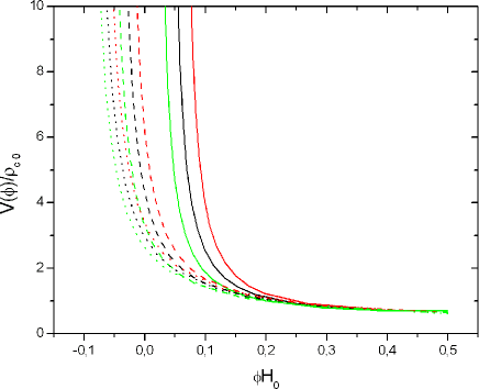
where $\rho_{c0}=3M_{Pl}^{2}H_{0}^{2}$, $E\left(z\right)$ is given by (14), $\omega_{\phi}\left(z\right)$ is given by (13) and $\Omega_{\phi}\left(z\right)$ is the solution of (11). From (16) and (15), we can compute $V(\phi)$. In figure 1, $V(\phi)$ is shown for some values of $\delta$ and $c$. Notice that, as we chose $\dot{\phi}$ positive, then $\phi$ evolves to the mininum of the potential. However, if we had chosen $\dot{\phi}$ negative, then because the right hand side of (15) would has the opposite sign, $V(\phi)$ would be now an increasing function of $\phi$ and again $\phi$ would evolve to the mininum of the potential.

Figure 1: Potential of tachyons $V(\phi)$, in units of $\rho_{c0}=3M_{Pl}^{2}H_{0}^{2}$. $\phi$ is in units of $H_{0}^{-1}$. The solid lines are for $c=0.85$, the dashed ones are for $c=1.1$ and the dotted are for $c=1.35$. For each value of $c$ the curves from right to left are for $\frac{\delta}{H_{0}}=-0.1$ (red), $\frac{\delta}{H_{0}}=0$ (black) and $\frac{\delta}{H_{0}}=+0.1$ (green), respectively.

The equation for evolution of $\phi$ (15) can be written in an integral form as

$$\Delta\phi=-\frac{1}{H_{0}}\int_{0}^{z}\frac{\sqrt{1+\omega_{\phi}\left(z\right)}}{E(z)(1+z)}dz\text{ .}$$

Since the model depends on $\Delta\phi$ - through $E\left(z\right)$ - and neither on $\phi$ nor on $\phi_{0}$, then it is independent of $\phi_{0}$. In other words, $\phi_{0}$ is not a parameter of the model and can be chosen arbitrarily. Therefore, the parameters of the model are $\delta$, $c$, $h$ and $\Omega_{\phi 0}$. Below, we discuss the comparison with observational data and the results obtained.

In lookback , the lookback time method has been discussed. Given an object $i$ at redshift $z_{i}$, its age $t(z_{i})$ is defined as the difference between the age of the universe at $z_{i}$ and the age of the universe at the formation redshift of the object, $z_{F}$, that is,

$$t(z_{i}) =H_{0}^{-1}\left[\int_{z_{i}}^{\infty}\frac{dz^{\prime}}{(1+z^{\prime})E(z^{\prime})}-\int_{z_{F}}^{\infty}\frac{dz^{\prime}}{(1+z^{\prime})E(z^{\prime})}\right]$$

$$=H_{0}^{-1}\int_{z_{i}}^{z_{F}}\frac{dz^{\prime}}{(1+z^{\prime})E(z^{\prime})}=t_{L}(z_{F})-t_{L}(z_{i})\text{ ,}$$ (17)

where $t_{L}$ is the lookback time, given by

$$t_{L}(z)=H_{0}^{-1}\int_{0}^{z}\frac{dz^{\prime}}{(1+z^{\prime})E(z^{\prime})}\text{ .}$$

Using (17), the observational lookback time $t_{L}^{obs}(z_{i})$ is

$$t_{L}^{obs}(z_{i}) =t_{L}(z_{F})-t(z_{i})=[t_{0}^{obs}-t(z_{i})]-[t_{0}^{obs}-t_{L}(z_{F})]$$

$$=t_{0}^{obs}-t(z_{i})-df\text{ ,}$$ (18)

where $t_{0}^{obs}$ is the estimated age of the universe today and $df$ is the delay factor,

$$df\equiv t_{0}^{obs}-t_{L}(z_{F})\ .$$

We now minimize $\chi_{lbt}^{2}$,

$$\chi_{lbt}^{2}=\sum_{i=1}^{N}\frac{[t_{L}(z_{i},\vec{p})-t_{L}^{obs}(z_{i})]^{2}}{\sigma_{i}^{2}+\sigma_{t_{0}^{obs}}^{2}}\text{ ,}$$

where $t_{L}(z_{i},\vec{p})$ is the theoretical value of the lookback time in $z_{i}$, $\vec{p}$ denotes the theoretical parameters, $t_{L}^{obs}(z_{i})$ is the corresponding observational value given by (18), $\sigma_{i}$ is the uncertainty in the estimated age $t(z_{i})$ of the object at $z_{i}$, which appears in (18) and $\sigma_{t_{0}^{obs}}$ is the uncertainty in getting $t_{0}^{obs}$. The delay factor $df$ appears because of our ignorance about the redshift formation $z_{F}$ of the object and has to be adjusted. Note, however, that the theoretical lookback time does not depend on this parameter, and we can marginalize over it.

In age35 and age32 the ages of 35 and 32 red galaxies are respectively given. For the age of the universe one can adopt $t_{0}^{obs}=13.73\pm 0.12Gyr$ wmap5yr . Although this estimate for $t_{0}^{obs}$ has been obtained assuming a $\Lambda CDM$ universe, it does not introduce systematical errors in the calculation: any systematical error eventually introduced here would be compensated by the adjust of $df$, in (18). On the other hand, such an estimate is in perfect agreement with other estimates, which are independent of the cosmological model, as for example $t_{0}^{obs}=12.6_{-2.4}^{+3.4}Gyr$, obtained from globular cluster ages krauss and $t_{0}^{obs}=12.5\pm 3.0Gyr$, obtained from radioisotopes studies cayrel .

For the cosmic radiation shift parameter in the flat universe we have

$$R=\sqrt{\Omega_{M}}\int_{0}^{z_{ls}}\frac{dz^{\prime}}{E(z^{\prime})}\ ,$$

where $z_{ls}$ is the last scattering surface redshift parameter. The value $R$ has been estimated from the 5-years WMAP wmap5yr results as $R_{obs}=1.715\pm 0.021$, for the flat universe, with $z_{ls}=1090.5\pm 1.0$ and is very weakly model dependent R . Thus we add to $\chi^{2}$ the term

$$\chi_{CMB}^{2}=\frac{\left(R-R_{obs}\right)^{2}}{\sigma_{R}^{2}}\ \text{.}$$

Baryonic Acoustic Oscilations (BAO) are described in terms of the parameter

$$A=\sqrt{\Omega_{M}}E(z_{BAO})^{-1/3}\left[\frac{1}{z_{BAO}}\int_{0}^{z_{BAO}}\frac{dz^{\prime}}{E(z^{\prime})}\right]^{2/3}\text{ ,}$$

where $z_{BAO}=0.35$. It has been estimated that $A_{obs}=0.493\pm 0.017$ BAO1 . We thus add to $\chi^{2}$ the term

$$\chi_{BAO}^{2}=\frac{\left(A-A_{obs}\right)^{2}}{\sigma_{A}^{2}}\ \text{.}$$

The BAO distance ratio $r_{BAO}\equiv D_{V}\left(z=0.35\right)/D_{V}\left(z=0.20\right)=1.812\pm 0.060$, estimated from the joint analysis of the 2dFGRS and SDSS data BAO2 , has also been included. It was demonstrated in BAO2 that this quantity is weakly model dependent. The quantity $D_{V}\left(z_{BAO}\right)$ is given by

$$D_{V}\left(z_{BAO}\right)=c\left[\frac{z_{BAO}}{H\left(z_{BAO}\right)}\left(\int_{0}^{z_{BAO}}\frac{dz^{\prime}}{H\left(z^{\prime}\right)}\right)^{2}\right]^{1/3}\text{ .}$$

So we have the contribution

$$\chi_{r_{BAO}}^{2}=\frac{\left(r_{BAO}-r_{BAO}^{obs}\right)^{2}}{\sigma_{r_{BAO}}^{2}}\text{ .}$$

Finally, we add the 397 supernovae data from Constitution compilation constitution . Defining the distance modulus

$$\mu(z)=5log_{10}\left[c(1+z)\int_{0}^{z}\frac{dz^{\prime}}{E(z^{\prime})}\right]+25-5log_{10}H_{0}\text{ ,}$$

we have the contribution

$$\chi_{SN}^{2}=\sum_{j=1}^{397}\frac{[\mu(z_{j})-\mu_{obs}(z_{j})]^{2}}{\sigma_{j}^{2}}\text{ .}$$

Using the expression $\chi^{2}=\chi_{lbt}^{2}+\chi_{CMB}^{2}+\chi_{BAO}^{2}+\chi_{r_{BAO}}^{2}+\chi_{SN}^{2}$, the likelihood function is given by

$$\mathcal{L}(\delta,c,h,\Omega_{\phi_{0}})\propto exp[-\frac{\chi^{2}(\delta,c,h,\Omega_{\phi_{0}})}{2}]\ \text{.}$$

In table 1 we present the values of the individual best fit parameters, with respective $1\sigma$, $2\sigma$ and $3\sigma$ confidence intervals.

Table 1: Values of the model parameters from lookback time, BAO, CMB and SNe Ia.

$\frac{\delta}{H_{0}}$ $-0.066\pm 0.092\pm 0.185\pm 0.277$ $c$ $0.865_{-0.022-0.035-0.045}^{+0.056+0.141+0.260}$ $\Omega_{\phi 0}$ $0.720\pm 0.016\pm 0.033\pm 0.049$ $h$ $0.666\pm 0.013\pm 0.026\pm 0.038$

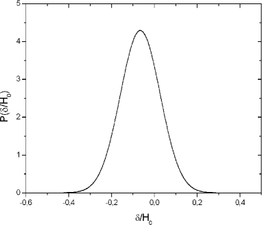
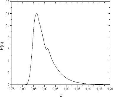
The figures 2 and 3 show the marginalized probability distributions for $\delta$ and $c$. The coupling constant $\delta$ is compatible with zero within $1\sigma$ level. Therefore, in this work it was not found evidence for interaction. However, the best fit value is of same order of magnitude obtained in a previous work, where the interacting tachyon model with power law potential has been considered sandro2 . $\Omega_{\phi 0}$ corresponds to a density matter parameter today $\Omega_{m0}=0.280\pm 0.016$, in perfect agreement with cosmological model independent estimatives, as for example $\Omega_{Mobs}=0.28\pm 0.04$ riess . The value of $h=0.666\pm 0.013$ is also in excellent agreement with observational values, independent of cosmological model ($h_{obs}=0.69\pm 0.12$ age35 and $h_{obs}=0.72\pm 0.08$ key ).

Figure 2: Probability distribuction of $\delta$.

Figure 3: Probability distribuction of $c$.

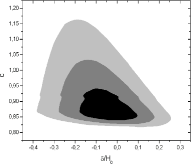
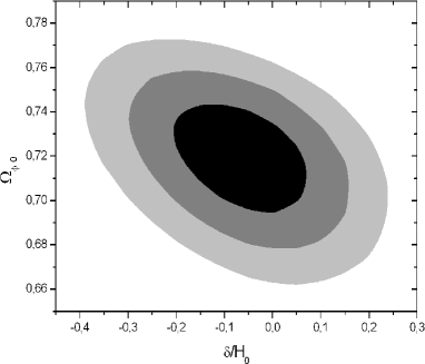
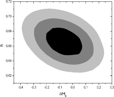
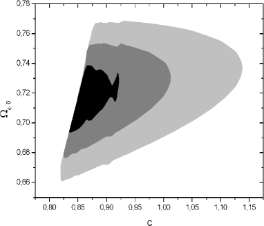
Figure 4: Confidence regions of $1\sigma$, $2\sigma$ and $3\sigma$ for two parameters.

Figure 4 shows the joint confidence regions for two parameters. As we can see, there is little degeneracy between the parameters of the model. In the confidence regions for $\delta$ versus $c$ and for $c$ versus $\Omega_{\phi 0}$, we see that there is a lower limit on $c$ $\approx 0.8$. This also can be seen in the marginalized probability distribution of $c$, which dies for $c\lesssim 0.85$. This lower limit is explained by the condition $\frac{\sqrt{\Omega_{\phi 0}}}{c}<1$, necessary for $\omega_{\phi}$ to be real and $\omega_{\phi}>-1$, discussed above. This limit can be seen more clearly in $c$ versus $\Omega_{\phi 0}$ confidence regions. Moreover, we have $c\simeq\sqrt{\Omega_{\phi 0}}$ for the best fit values of these parameters. This implies that $\omega_{\phi 0}\simeq-1$ and the model approaches $\Lambda CDM$ today. This is consistent with the fact that, as $\Lambda CDM$ fits all observational data, then any alternative model must not deviates much from $\Lambda CDM$ for $z\approx 0$. 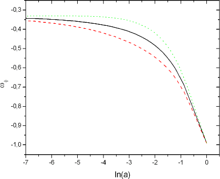However, for $z>0$, the model is qualitatively different from $\Lambda CDM$, as $\omega_{\phi}$ approximates $-1/3$, see figure 5.

We have obtained $c<1$ at $1\sigma$ confidence level. As already said above, this implies that the equation of state parameter $\omega_{\phi}$ will not be real for all future times. However, this is not a very serious problem, because $c$ is compatible with values above unit at $2\sigma$ confidence level. Moreover, one could say that $c<1$ is only an effect due to lack of more precise observational data. Anyway, the very simple model presented here is expected to be only an effective description of a more sophisticated subjacent theory of dark energy. In principle, nothing guarantees that it will be a good description for all future times.

Figure 5: Equation of state parameter of dark energy $\omega_{\phi}(a)$, for $c=0.85$ and $\frac{\delta}{H_{0}}=-0.1$ (red dashed line), $\frac{\delta}{H_{0}}=0$ (black solid line) and $\frac{\delta}{H_{0}}=+0.1$ (green dotted line).

In summary, a combination of holographic dark energy model and interacting tachyon field was implemented. It was showed that it is possible to fix the potential of interacting tachyon by imposing that the energy density of the tachyons must match the energy density of the holographic dark energy. A comparison of the model with recent observational data was made and the coupling is consistent with zero. However, in a previous work sandro2 with interacting tachyons with power law potential, a non-vanishing coupling constant had been obtained with $90\%$ of confidence. So the possibility of a small, but calculable, interaction in the dark sector remains open, and future investigations, with more realistic models and more observational data are necessary to solve this question.

This work has been supported by CNPq (Conselho Nacional de Desenvolvimento Científico e Tecnológico) of Brazil. We would like to thank E. Abdalla for suggestions and useful comments and Y. Gong for useful conversations.

References

(1)
(2)W. Zimdahl and D. Pavon Phys. Lett. B521 (2001)
133; L. P. Chimento, A. S. Jakubi, D. Pavon and W. Zimdahl Phys. Rev.
D67 (2003) 083513.
(3)B. Gumjudpai, T. Naskar, M. Sami and S. Tsujikawa JCAP06 (2005) 007; M. R. Setare, Phys. Lett.B642
(2006) 1; Eur. Phys. J. C50 (2007) 991; R. Rosenfeld
Phys. Rev. D75 (2007) 083509; M. Quartin, M. O. Calvao, S.
E. Joras, R. R. R. Reis and I. Waga JCAP05 (2008) 007; Q.
Wu, Y. Gong, A. Wang and J.S. Alcaniz Phys. Lett. B659
(2008) 34; M.R. Setare and E. C. Vagenas Phys. Lett. B666
(2008) 111.
(4)B. Wang, Y.-G. Gong and E. Abdalla, Phys. Lett.B624 (2005) 141.
(5)J.-H. He and B. Wang JCAP06 (2008) 010; C.
Feng, B. Wang, E. Abdalla and R.-K. Su Phys. Lett. B665
(2008) 111; J.-H. He, B. Wang and E. Abdalla, Phys. Lett. B671
(2009), 139.
(6)M. Jamil, M. A. Rashid Eur. Phys. J. C56 (2008)
429; Eur. Phys. J. C58 (2008) 111; M.R. Setare and E. C.
Vagenas, Int. J. Mod. Phys. D 18 (2009) 147; X.-M. Chen,
Y.-G. Gong and E. N. Saridakis,JCAP 04 (2009) 001; Z.-K.
Guo, N. Ohta and S. Tsujikawa, Phys. Rev.D76 (2007) 023508;
O. Bertolami, F. Gil Pedro and M. Le Delliou, Phys. Lett.
B654 (2007) 165; O. Bertolami, F.Gil Pedro and M.Le Delliou,
Gen. Rel. Grav. 41 (2009) 2839.
(7)E. Abdalla and B. Wang Phys. Lett. B651 (2007) 89.
(8)B. Wang, J. Zang, C.-Y. Lin, E. Abdalla and S. Micheletti,
Nucl. Phys. B778 (2007) 69.
(9)S. Micheletti, E. Abdalla and B. Wang, Phys. Rev.
D79 (2009) 123506.
(10)P. J. E. Peebles, Physical Cosmology, (Princeton U.
Press, 1993).
(11)E. Abdalla, L. R. W. Abramo, L. Sodre, Jr. and B. Wang,
Phys. Lett.B673, (2009) 107; E. Abdalla, L. R. W. Abramo
and J. C. C. de Souza, 0910.5236 [gr-qc].
(12)L. Amendola Phys. Rev. D62 (2000) 043511;
R. Bean, E. E. Flanagan, I. Laszlo and M. Trodden Phys. Rev. D78 (2008) 123514.