Comparison of dark energy models: A perspective from the latest observational data
Abstract
In this paper, we compare some popular dark energy models under the assumption of a flat universe by using the latest observational data including the type Ia supernovae Constitution compilation, the baryon acoustic oscillation measurement from the Sloan Digital Sky Survey, the cosmic microwave background measurement given by the seven-year Wilkinson Microwave Anisotropy Probe observations and the determination of from the Hubble Space Telescope. Model comparison statistics such as the Bayesian and Akaike information criteria are applied to assess the worth of the models. These statistics favor models that give a good fit with fewer parameters. Based on this analysis, we find that the simplest cosmological constant model that has only one free parameter is still preferred by the current data. For other dynamical dark energy models, we find that some of them, such as the dark energy, constant , generalized Chaplygin gas, Chevalliear-Polarski-Linder parametrization, and holographic dark energy models, can provide good fits to the current data, and three of them, namely, the Ricci dark energy, agegraphic dark energy, and Dvali-Gabadadze-Porrati models, are clearly disfavored by the data.
pacs:
98.80.-k, 95.36.+x, 98.80.EsI Introduction
Dark energy has become one of the most important issues of the modern cosmology ever since the observations of type Ia supernovae (SNe Ia) first indicated that the universe is undergoing an accelerated expansion at the present stage [1]. However, hitherto, we still know little about dark energy. The limited information we know about dark energy includes: it causes the cosmic acceleration; it accounts for two-thirds of the cosmic energy density; it is gravitationally repulsive; it does not appear to cluster in galaxies; and so on. Many cosmologists suspect that the identity of dark energy is the cosmological constant that fits the observational data well. While, one also has reason to dislike the cosmological constant since it always suffers from the theoretical problems such as the “fine-tuning” and “cosmic coincidence” puzzles [2]. The fine-tuning problem, also known as the “old cosmological constant problem,” is motivated by the enormous discrepancy between the theoretical prediction for the cosmological constant and its measured value. The so-called “new cosmological constant problem,” namely, the cosmic coincidence problem, questions why we just live in an era when the densities of dark energy and matter are almost equal, which also indicates that the cosmological constant scenario may be incomplete. Thus, a variety of proposals for dark energy have emerged.
The possibility that dark energy is dynamical, for example, in a form of some light scalar field [3], has been explored by cosmologists for a long time. A basic way to explore such a dynamical dark energy model in light of observational data is to parameterize dark energy by an equation-of-state parameter , relating the dark energy pressure to its density via . In general, this parameter is time variable. The most commonly used forms of involve the constant equation of state, , and the Chevalliear-Polarski-Linder form [4], , where and parameterize the present-day value of and the first derivative. There are also many other dynamical dark energy models which stem from different aspects of new physics. For example, the “holographic dark energy” models [5, 6, 7, 8, 9, 10, 11] arise from the holographic principle of quantum gravity theory, and the Chaplygin gas models [12, 13, 14] are motivated by brane world scenarios and may be able to unify dark matter and dark energy. In addition, there is also significant interest in modifications to general relativity, in the context of explaining the acceleration of the universe. The Dvali-Gabadadze-Porrati models [15, 16, 17] arise from a class of brane-related theories in which gravity leaks out into the bulk at large distances, leading to the accelerated expansion of the universe.
In the face of so many competing dark energy candidates, it is important to find an effective way to decide which one is right, or at least, which one is most favored by the observational data. Although the accumulation of the current observational data has opened a robust window for constraining the parameter space of dark energy models, the model filtration is still a difficult mission owing to the accuracy of current data as well as the complication caused by different parameter numbers of various dark energy models. In this paper, we make an effort to assess some popular dark energy models in light of the latest observational data, including the Constitution SN data [18] and other cosmological probes such as the distance information measured by Wilkinson Microwave Anisotropy Probe (WMAP) [19], and the Baryon Acoustic Oscillations (BAO) [20, 21]. To make a comparison for various dark energy models with different numbers of parameters and decide on the model preferred by the current data, following Ref. [22], we apply model comparison statistics such as the Bayesian information criterion (BIC) [23] and the Akaike information criterion (AIC) [24] in our analysis.
This paper is organized as follows. In Sec. II, we discuss the information criteria in the context of dark energy model selection. In Sec. III, we give details of the observational data sets used. Section IV describes nine popular dark energy models and assesses which one is preferred by the current data. The results are discussed in Sec. V.
II Methodology
In this work we employ the statistics. For a physical quantity with experimentally measured value , standard deviation , and theoretically predicted value , the value is given by
| (1) |
The total is the sum of all s, i.e.,
| (2) |
The observational data we use in this paper include the Constitution SN Ia sample, the Cosmic Microwave Background (CMB) measurement given by the seven-year WMAP observations, the BAO measurement from the Sloan Digital Sky Survey (SDSS), and the measurement of from the Hubble Space Telescope (HST) [25].
However, the statistic alone cannot provide effective way to make a comparison between competing models since this method is based on the assumption that the underlying model is the correct one. The statistics is good at finding the best-fit values of parameters but is insufficient for deciding whether the model itself is the best one. Since in general a model with more parameters tends to give a lower , it is unwise to compare different models by simply considering with likelihood contours or best-fit parameters. Instead, one may employ the information criteria (IC) to assess different models, which is also based on a likelihood method. In this paper, we use the BIC [23] and AIC [24] as model selection criteria. According to these criteria, models that give a good fit with fewer parameters will be more favored. So, these criteria embody the principle of Occam’s razor, “entities must not be multiplied beyond necessity.” The applications of the BIC and AIC in a cosmological context can be found in, e.g., Refs. [26, 27].
The BIC, also known as the Schwarz information criterion [23], is given by
| (3) |
where is the maximum likelihood, is the number of parameters, and is the number of data points used in the fit. Note that for Gaussian errors, , and the difference in BIC can be simplified to . A difference in BIC () of 2 is considered positive evidence against the model with the higher BIC, while a of 6 is considered strong evidence.
The AIC [24] is defined as
| (4) |
which gives results similar to the BIC approach, but it should be pointed out that the AIC is more lenient than BIC on models with extra parameters for any likely data set . Also, in this case, the absolute value of the criterion is not of interest, only the relative value between different models, , is useful. As mentioned in Ref. [28], there is a version of the AIC corrected for small sample sizes, , which is important for . Obviously, in our case, this correction is negligible.
It should be noted that the information criteria alone can at most say that a more complex model is not necessary to explain the current data, since a poor information criterion result might arise from the fact that the current data are too poor to constrain the extra parameters in this complex model, and it might become preferred with improved data. Actually, this is just the current situation for dynamical dark energy models.
A more sophisticated method for model selection is provided by the Bayesian evidence which does not simply count parameters, but considers how much the allowed volume in data space increases due to the addition of extra parameters, as well as any correlations between the parameters. So, the Bayesian evidence requires an integral of the likelihood over the whole model parameter space, which may be lengthy to calculate, but avoids the approximations used in the information criteria and also permits the use of prior information if required. This method has been applied in a variety of cosmological contexts; see, e.g., Refs. [29, 30, 31]. Information criteria require no assumptions for the prior or the metric on the space of model parameters. In this paper, we will use the first approximation provided by the information criteria without calculating the full Bayesian evidence. This simpler version is sufficient for our purpose.
III Current Observational Data
In order to test the different dark energy models, we have used the observational data currently available. In this section, we describe how we use these data.
III.1 Type Ia supernovae
Up to now, SNe Ia provide the most direct indication of the accelerated expansion of the universe. It is commonly believed that these SNe Ia all have the same intrinsic luminosity, and thus they are used as “standard candles.” Therefore, measuring both their redshift and their apparent peak flux gives a direct measurement of their luminosity distance as a function of redshift . The function encodes the expansion history of the universe so that by which the information of dark energy can be extracted.
In this paper, for the SN Ia data, we use the Constitution sample including 397 data that are given in terms of the distance modulus compiled in Table 1 of Ref. [18]. The theoretical distance modulus is defined as
| (5) |
where with the Hubble constant in units of 100 km/s/Mpc, and the Hubble-free luminosity distance is
| (6) |
where , is the fractional curvature density at , and
The for the SN data is
| (7) |
where and are the observed value and the corresponding 1 error of distance modulus for each supernova, respectively, and denotes the model parameters.
What should be mentioned is that since the absolute magnitude of a supernova is unknown, the degeneracy between the Hubble constant and the absolute magnitude implies that one cannot quote constraints on either one. Thus the nuisance parameter in SN data is not the observed Hubble constant and is different from that in the BAO and CMB data. Therefore we should analytically marginalize over in the SN data.
III.2 Baryon Acoustic Oscillations
Aside from the SN data, the other external astrophysical results that we shall use in this paper for the joint cosmological analysis are the BAO and CMB data. First, we describe how we use the BAO data. The BAO is a powerful probe of dark energy, since it can be used to measure not only the angular diameter distance through the clustering perpendicular to the line of sight, but also the expansion rate of the universe through the clustering along the line of sight. However, the current data are not accurate enough to allow us to extract and separately. Actually, the BAO currently can barely be measured in the spherically-averaged correlation function [33].
The spherical average gives us the following effective distance measure [34]
| (13) |
where is the proper (not comoving) angular diameter distance,
| (14) |
The BAO data from the spectroscopic SDSS Data Release 7 (DR7) galaxy sample [21] give . Thus, the for BAO data is,
| (15) |
III.3 Cosmic Microwave Background
The CMB is sensitive to the distance to the decoupling epoch via the locations of peaks and troughs of the acoustic oscillations. In this paper, we employ the “WMAP distance priors” given by the seven-year WMAP observations [19]. This includes the “acoustic scale” , the “shift parameter” , and the redshift of the decoupling epoch of photons .
The acoustic scale describes the distance ratio , defined as
| (16) |
where a factor of arises because is the proper angular diameter distance, whereas is the comoving sound horizon at . The fitting formula of is given by
| (17) |
where and are the present-day baryon and photon density parameters, respectively. In this paper, we fix (for K) and , which are the best-fit values given by the seven-year WMAP observations [19]. We use the fitting function of proposed by Hu and Sugiyama [36]:
| (18) |
where
| (19) |
The shift parameter is responsible for the distance ratio , given by [37]
| (20) |
Actually, this quantity is different from by a factor of , and also ignores the contributions from radiation, curvature, or dark energy to . Nevertheless, we still use to follow the convention in the literature.
Following Ref. [19], we use the prescription for using the WMAP distance priors. Thus, the for the CMB data is
| (21) |
where is a vector, and is the inverse covariance matrix. The seven-year WMAP observations [19] give the maximum likelihood values: , , and . The inverse covariance matrix is also given in Ref. [19]:
| (22) |
III.4 Hubble constant
In this paper we also use the prior on the present-day Hubble constant, km/s/Mpc [25]. In Ref. [25], the authors obtain this measurement result of from the magnitude-redshift relation of 240 low- type Ia supernovae at . The absolute magnitudes of these supernovae are calibrated by using new observations from HST of 240 Cepheid variables in six local type Ia supernovae host galaxies and the maser galaxy NGC 4258. It is remarkable that this Gaussian prior on has also been used in the analysis of WMAP 7-year observational data [19]. The function for the Hubble constant is
| (23) |
III.5 Combining the constraints
Since the SN, BAO, CMB and are effectively independent measurements, we can combine our results by simply adding together the functions. Thus, we have
| (24) |
Note that and are free of , while and are still relevant to .
IV Dark Energy Models
In the standard homogeneous and isotropic Friedmann-Robertson-Walker (FRW) universe, the Friedmann equation is expressed as
| (25) |
where is the reduced Planck mass, is the total energy density containing contributions from cold dark matter, baryons, radiations, and dark energy, and describes the spatial geometry of the universe. Usually, the properties of dark energy, such as its equation of state parameter , are degenerate with the spatial curvature of the universe . Thus, although in principle one should include as an additional parameter when fitting dark energy models in light of observational data, the current data are not accurate enough to distinguish between and , owing to the degeneracy of them. On the other hand, it is well known that most inflation models in which the inflationary periods last for much longer than 60 -folds predict a spatially flat universe, . Actually, the inflation theory has become a paradigm in the modern cosmology and it has received strong support from the CMB observations. Under such circumstances, therefore, in this paper we shall use a “strong inflation prior,” imposing a flatness prior, and explore dark energy models in the context of such inflation models.
In a spatially flat FRW universe , the Friedmann equation (25) reduces to
| (26) |
where , and are the present-day densities of dust matter, radiation and dark energy, respectively, and is given by the specific dark energy models. This equation is usually rewritten as
| (27) |
Note that the radiation density parameter is the sum of the photons and relativistic neutrinos [35],
| (28) |
where is the effective number of neutrino species, and in this paper we take its standard value 3.04 [19]. In some cases, the evolution of the dark energy density parameter is determined by a differential equation, and thus one should express the Friedmann equation as
| (29) |
In what follows, we choose nine popular dark energy models and examine whether they are consistent with the data currently available to us. We divide these models into five classes:
-
1.
Cosmological constant model.
-
2.
Dark energy models with equation of state parameterized.
-
3.
Chaplygin gas models.
-
4.
Holographic dark energy models.
-
5.
Dvali-Gabadadze-Porrati (DGP) brane world and related models
It should be mentioned that the dark energy models discussed in this paper involve those invoke a variation in the equations governing gravity, say, the DGP model. Actually, in some cases the two are interchangeable descriptions of a single theory, albeit they might affect the structure growth in different manners (see, e.g., Refs. [38, 39]). In this paper, we ignore the exiguous difference between them, and call them uniformly the “dark energy models.” The models discussed and the parameters that describe each model are summarized in Table 1. Note that when fitting the data there is an additional parameter, , which is not considered as a model parameter but is included in when calculating AIC and BIC. The fit and information criteria results are summarized in Table 2.
Next, we shall outline the basic equations describing the evolution of the cosmic expansion in each of the competing dark energy models, calculate the best-fit values of their parameters, and find their corresponding , AIC and BIC values.
| Model | Abbreviation111The abbreviations used in Table 2 and Fig. 10. | Model parameters222The free parameters in each model. Note that the additional parameter appearing in the data fits is not considered as a model parameter but is included in when calculating AIC and BIC. | Number of model parameters () |
|---|---|---|---|
| Cosmological constant | 1 | ||
| Constant | , | 2 | |
| Chevallier-Polarski-Linder | CPL | , , | 3 |
| Generalized Chaplygin gas | GCG | , | 2 |
| Holographic dark energy | HDE | , | 2 |
| Agegraphic dark energy | ADE | 1 | |
| Ricci dark energy | RDE | , | 2 |
| Dvali-Gabadadze-Porrati | DGP | 1 | |
| Phenomenological extension of DGP | DE | , | 2 |
| Model | AIC | BIC | |
|---|---|---|---|
| 468.461 | 0 | 0 | |
| 468.327 | 1.866 | 5.862 | |
| DE | 468.452 | 1.991 | 5.987 |
| GCG | 468.461 | 2 | 5.996 |
| CPL | 467.663 | 3.202 | 11.195 |
| HDE | 470.513 | 4.052 | 8.048 |
| RDE | 493.772 | 27.311 | 31.308 |
| ADE | 503.039 | 34.578 | 34.578 |
| DGP | 530.443 | 61.982 | 61.982 |
| 00footnotetext: Notes: The cosmological constant model is preferred by both the AIC and the BIC. Thus, the AIC and BIC values for all other models in the table are measured with respect to these lowest values. The models are given in order of increasing AIC. |
IV.1 Cosmological constant model
The cosmological constant was first introduced by Einstein [40] with a wrong motivation, but nowadays it has become the most promising candidate for dark energy responsible for the current cosmic acceleration. While it has been suffering from the theoretical problems, it can explain the observations well. The cosmological model containing a cosmological constant and cold dark matter (CDM) component is usually called CDM model in the literature. The unique feature of the cosmological constant is that its equation-of-state parameter has the value at all times, so in this model we have
| (30) |
It is obvious that this model is a one-parameter model, with the sole independent parameter .
The best-fit values of parameters (including the model parameter and the dimensionless Hubble parameter ) and the corresponding are:
| (31) |
This model has the lowest values of AIC and BIC in all the models tested, so AIC and BIC are measured with respect to this model; see Table 2.
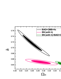
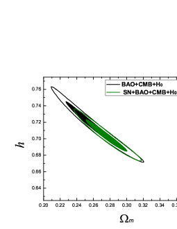
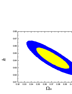
To make a comparison, we refer to Ref. [19] in which Komatsu et al. give the best-fit parameters: and , for the flat CDM model from WMAP 7-year data combined with BAO and data. We find that our results with SN Constitution data are consistent with this result. We also stress that in the joint data analysis we have used the chi square of SN data that is -free, instead of that is -relevant. For making a clear comparison, we also perform a joint analysis with the -relevant SN chi square , and in this way we find the best-fit parameters: and , with , in accordance with the results of Ref. [41]. Such a big implies that this way does not seem to be correct. Figure 1 shows the probability contours in the plane for the flat CDM model. The left panel tells us that if we use the -relevant , a great tension will be brought between the SN limit and the BAO+CMB limit, and the right panel shows that the tension will disappear when considering the -free . Actually, in Ref. [42], Wang and Mukherjee have argued that because of calibration uncertainties, SN data need to be marginalized over if SN data are combined with data that are sensitive to the value of . Our results further confirm this opinion.
IV.2 Dark energy models with equation of state parameterized
For this class, we consider two models: the constant parametrization and the Chevallier-Polarski-Linder (CPL) parametrization.
IV.2.1 Constant parametrization
In this case, the equation-of-state parameter of dark energy is assumed to be a constant, so in a flat universe we have
| (32) |
This is a two-parameter model with the model parameters and .
The best-fit parameters and the corresponding are:
| (33) |
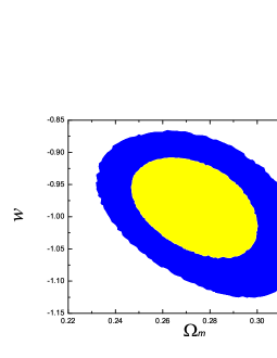
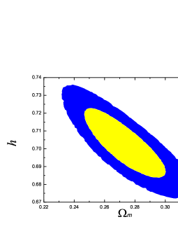
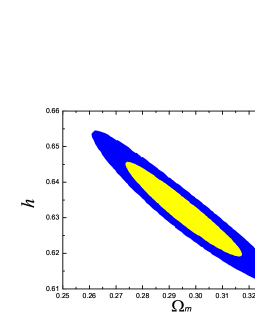
We plot the likelihood contours for this model in the and planes in Fig. 2. From this figure, we see that when the equation of state does not depend on redshifts, dark energy is consistent with a cosmological constant within 1 range. Comparing with the cosmological constant model, this model gives a lower , but due to one extra parameter it has, it is punished by the information criteria: and .
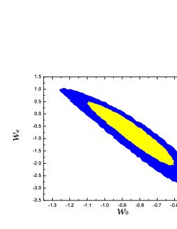
IV.2.2 Chevallier-Polarski-Linder parametrization
Now, we consider the commonly used CPL model [4], in which the equation of state of dark energy is parameterized as
| (34) |
where and are constants. The corresponding can be expressed as
| (35) |
There are three independent model parameters in this model: .
According to the joint data analysis, we find the best-fit parameters and the corresponding :
| (36) |
We plot the likelihood contours for the CPL model in the and planes in Fig. 3. We note that the best-fit parameters of the CDM model (, and ) still lie in the 1 regions of the CPL model, indicating that the CDM model is fairly consistent with the current observational data. Since the CPL model has three free model parameters, it should have made considerable improvement in the fit, however, it gives a nearly equal contrasting to the constant model (only smaller by 0.664). The differences in the information criteria with respect to the CDM model are: and . The information criteria result of CPL is worse than the model (especially its value is very large). This implies that the CPL model is too complex to be necessary in explaining the current data, comparing with the simpler models such as the model and the constant model.
IV.3 Chaplygin gas models
Chaplygin gas models describe a background fluid with that is commonly viewed as arising from the d-brane theory. Moreover, these models may be able to unify dark energy and dark matter. We should have considered both the original () and the generalized Chaplygin gas models, however, the original Chaplygin gas model [12] has been proven to be inconsistent with the observational data [22], we thus only consider the generalized Chaplygin gas (GCG) model [13] in this paper.
The GCG has an exotic equation of state:
| (37) |
where is a positive constant. This leads to the energy density of the GCG:
| (38) |
where . When , the GCG behaves like a dust matter; when , the GCG behaves like a cosmological constant. So, the GCG model is considered as a unification scheme of the cosmological constant and the CDM. In a flat universe, we have
| (39) |
This model has two independent model parameters: . The cosmological constant model is recovered for and .
The best-fit parameters and the corresponding are:
| (40) |
We find that for the GCG model the value is the same as that of the CDM model, which is an amazing coincidence. The best-fit value of is so close to zero, implying that the CDM limit of this model is favored. We plot the likelihood contours for the GCG model in the and planes in Fig. 4. As a two-parameter model, the GCG performs well under the information criteria tests: and .
IV.4 Holographic dark energy models
Holographic dark energy models arise from the holographic principle of quantum gravity. The holographic principle determines the range of validity for a local effective quantum field theory to be an accurate description of the world involving dark energy, by imposing a relationship between the ultraviolet (UV) and infrared (IR) cutoffs [43]. As a consequence, the vacuum energy becomes dynamical, and its density is inversely proportional to the square of the IR cutoff length scale that is believed to be some horizon size of the universe, namely, . In this subsection, we consider three holographic dark energy models: the original holographic dark energy (HDE) model [5], the agegraphic dark energy (ADE) model [8], and the holographic Ricci dark energy (RDE) model [10]. We note here that, different from the previous several models, the holographic dark energy models do not involve the cosmological constant model as a subclass.
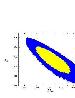
IV.4.1 Holographic dark energy model
The HDE model chooses the future event horizon size as its IR cutoff scale, so the energy density of HDE reads
| (41) |
where is a constant, and is the size of the future event horizon of the universe, defined as
| (42) |
In this case, is given by Eq. (29), where the function is determined by a differential equation:
| (43) |
where a prime denotes , and
| (44) |
with
| (45) |
The HDE model contains two independent model parameters: . Solving Eq. (43) numerically and substituting the resultant into Eq. (29), the corresponding can be obtained.
For this model, we obtain the best-fit parameters and the corresponding :
| (46) |
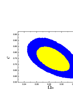
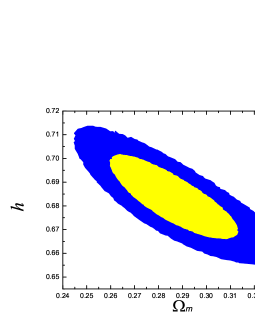
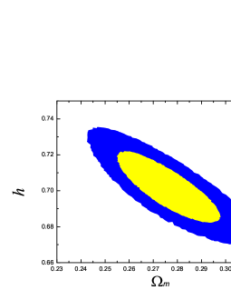
Our results are generally consistent with those derived in previous works [31, 44]. We plot the likelihood contours for the HDE model in the and planes in Fig. 5. The HDE model performs fine under the information criteria tests, with the results and . It should be stressed that the HDE model does not contain the CDM model as a sub-model, whereas other two-parameter models which perform better than the HDE model, such as the DE, constant , and GCG models, all nest the cosmological constant and tend to collapse to the CDM model once being up against the current observational data.
IV.4.2 Agegraphic dark energy model
The ADE model discussed in this paper is actually the new version of the ADE model [8] (sometimes called the new ADE model in the literature) which chooses the conformal age of the universe
| (47) |
as the IR cutoff, so the energy density of ADE is
| (48) |
where is a constant which plays the same role as in the HDE model.
As the same as the HDE model, is also given by Eq. (29), where the function is governed by the differential equation:
| (49) |
where the form of is the same as Eq. (44), in which
| (50) |
Following Ref. [46], we choose the initial condition, , at , and then Eq. (49) can be numerically solved. Substituting the resultant into Eq. (29), the function can be obtained. Note that in this model once is given, by solving Eq. (49), can be derived accordingly. So, actually, the ADE model is a one-parameter model; the sole model parameter is .
For this model, we get the best-fit parameters and the corresponding :
| (51) |
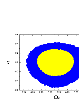
This leads to . We plot the likelihood contours for the ADE model in the plane in Fig. 6. As a single-parameter model, the ADE performs much worse than the CDM model: its is greater than that of the CDM model by about 30, and its .
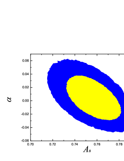
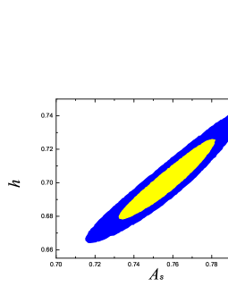
IV.4.3 Ricci dark energy model
In the RDE model, the IR cutoff length scale is given by the average radius of the Ricci scalar curvature , so in this case we have . In a flat universe, the Ricci scalar is , and as suggested in Ref. [10], the energy density of RDE reads
| (52) |
where is a positive constant. From the Friedmann equation, we derive
| (53) |
where . Solving this differential equation, we get the following form:
| (54) |
This is a two-parameter model, and its free model parameters are: .
For the RDE model, the best-fit parameters and the corresponding are:
| (55) |
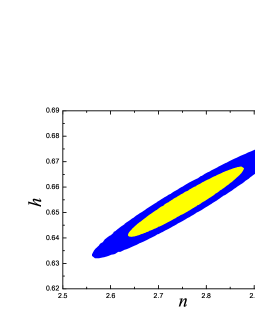
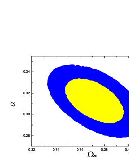
We plot the likelihood contours for the RDE model in the and planes in Fig. 7. Like the ADE model, RDE also performs very bad: and . This conclusion is consistent with the previous work [31, 45].
IV.5 Dvali-Gabadadze-Porrati brane world and related models
The DGP brane world model is a well-known example of the modification of general relativity for explaining the acceleration of the universe. In this subsection, we consider two models: the DGP model [15] and its phenomenological extension (namely, the dark energy model) [17].
IV.5.1 Dvali-Gabadadze-Porrati model
The DGP model arises from the brane world theory in which gravity leaks out into the bulk at large scales, resulting in the possibility of an accelerated expansion of the universe. In this model, the Friedmann equation is modified as
| (56) |
where is the crossover scale. In this model, is given by
| (57) |
where is a constant. The flat DGP model only contains one free model parameter, .
For the DGP model, the best-fit parameters and the corresponding are:
| (58) |
We plot the likelihood contours for the DGP model in the plane in Fig. 8. We see that the DGP model, as a single-parameter model, is even worse than the ADE model under the observational tests. Its is greater than that of the ADE model by about 30, and it yields , also much larger than all other models we considered. So, the fitting result shows that the DGP model seems to be inconsistent with the current observational data (see also Ref. [22]).
What should be mentioned is that the DGP model could perform much better when considering the systematic errors of the SN Ia data. For example, using the MLCS2k2 light-curve fitter for the SNe Ia data, the authors of Ref. [47] found that the DGP model performs better than the standard CDM model. Currently the SNe Ia measurement errors are being dominated by systematic rather than statistical uncertainties, and for the sake of simplicity we would not discuss this problem in this paper. See Refs. [18, 47, 48, 49] for detailed discussions of this issue.
IV.5.2 Phenomenological extension of DGP: dark energy model
Inspired by the DGP brane world model in which the Friedmann equation is modified, Dvali and Turner [17] proposed a phenomenological dark energy model, sometimes called the dark energy model, which interpolates between the pure CDM model and the DGP model with an additional parameter . In this model, the Friedmann equation is modified as
| (59) |
where is a phenomenological parameter, and . According to this Friedmann equation, is determined by the following equation:
| (60) |
So, this model is a two-parameter model, with the independent model parameters . Note that corresponds to the DGP model and corresponds to the cosmological constant model.
Our joint analysis shows that for the DE model the best-fit parameters and the corresponding are:
| (61) |
We plot the likelihood contours for the DE model in the and planes in Fig. 9. We notice that the best-fit value of deviates one evidently, implying that the DGP model is incompatible with the current observational data. The cosmological constant limit, , is consistent with this model within 1 range. Moreover, we find that the DE model gives the smaller than the model under our investigation, and its information criteria results, and , also indicate that the DE model fares the best, except for the CDM and models, under the current observational tests.
V Discussion and Conclusion
In this work, we have considered nine popular dark-energy cosmological models and tested them against the latest cosmological data. This includes observational data of SNe Ia from the Constitution compilation, BAO from the SDSS, the CMB “WMAP distance priors” from the WMAP seven-year observations, and the measurement of from the HST. We have used the “strong inflation prior” that imposes a flatness prior, and explored dark energy models in the context of such a flat universe assumption. To assess the various competing dark energy models and make a comparison, we have applied the information criteria, both the BIC and AIC, in this analysis.
For each model, we have outlined the basic equations governing the evolution of the universe, calculated the best-fit values of its parameters, and found its and values. Table 1 summarizes all the models under consideration and the parameters that describe each model. We have plotted the likelihood contours of parameters for all the models. The fit and information criteria results have been summarized in Table 2. Note that since the cosmological constant model has the lowest values of both AIC and BIC, the values of and are measured with respect to this model.
From Table 1, we see that according to the number of parameters the models can be divided into three classes: the one-parameter models, including , ADE, and DGP models; the two-parameter models, including , GCG, HDE, RDE, and DE models; and the three-parameter model, namely, the CPL model. If we only compare , we find that the model is not the best one, and there are four models, namely, DE, , GCG, and CPL models, a little bit better than the model according to this criterion. However, if the economical efficiency is considered, one will find that the model is the best one to explain the current data, since both the AIC and BIC values it yields are the smallest. Although the CPL model can fit the current data well and has the lowest , it is too complex (it has three free model parameters) to be necessary, yet. In the two-parameter models, the model performs best in explaining the current data.
We can also classify these models in another way that whether the model can reduce to the model. Some models, such as , CPL, GCG, and DE, can reduce to the model, but the other ones, namely, HDE, ADE, RDE, and DGP, can not. From Table 2, we see that the models nest the all perform well, whereas the models that cannot reduce to the perform illy, except for the HDE model. The HDE model has the ability in explaining the current data nearly as good as DE, , and GCG that nest the . Also, we notice that although the DE, , GCG, and CPL models can fit the data well, they actually all tend to collapse to the model with their best-fit parameters.
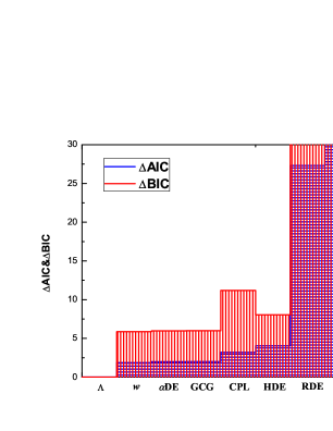
Out of all the candidate models we consider, it is obvious that the simplest model remains the best one. Following it are a series of models that give comparably good fits but have more free parameters. These include the DE, , GCG, and HDE models, which have two free parameters; and the CPL model, which has three free parameters. We have shown that the DE, , GCG, and CPL models can reduce to the model and their best-fit parameters indeed do so (to within 1 ranges). The HDE model is the sole one that can give a good fit but does not nest . The last three models in Table 2, RDE, ADE, and DGP, are clearly disfavored. They have fewer parameters than models like CPL, but they score poorly because they are unable to provide a good fit to the data. They cannot reduce to the model for any values of their parameters. We provide a graphical representation of the IC results in Fig. 10 which directly shows the scores (in the AIC and BIC tests) the models gain.
In conclusion, given the current quality of the observational data, and with the assumption of a flat universe, information criteria indicate that the cosmological constant model is still the best one and there is no reason to prefer any more complex model. This conclusion is in accordance with the previous work by Davis et al. [22]. We look forward to seeing whether this conclusion could be changed by future more accurate data.
Acknowledgements.
We would like to thank Yun-Gui Gong, Shuang Wang and Tower Wang for helpful discussions and suggestions. This work was supported by the Natural Science Foundation of China under Grant Nos. 10705041, 10821504, 10975032 and 10975172, and Ministry of Science and Technology 973 program under Grant No. 2007CB815401.References
-
[1]
A. G. Riess et al. [Supernova Search Team Collaboration],
Observational Evidence from Supernovae for an Accelerating Universe and a
Cosmological Constant,
Astron. J. 116, 1009 (1998)
[arXiv:astro-ph/9805201];
S. Perlmutter et al. [Supernova Cosmology Project Collaboration], Measurements of and from 42 High-Redshift Supernovae, Astrophys. J. 517, 565 (1999) [arXiv:astro-ph/9812133]. -
[2]
S. Weinberg,
The cosmological constant problem,
Rev. Mod. Phys. 61, 1 (1989);
V. Sahni and A. A. Starobinsky, The Case for a Positive Cosmological Lambda-term, Int. J. Mod. Phys. D 9, 373 (2000) [arXiv:astro-ph/9904398];
S. M. Carroll, The cosmological constant, Living Rev. Rel. 4, 1 (2001) [arXiv:astro-ph/0004075];
P. J. E. Peebles and B. Ratra, The cosmological constant and dark energy, Rev. Mod. Phys. 75, 559 (2003) [arXiv:astro-ph/0207347];
T. Padmanabhan, Cosmological constant: The weight of the vacuum, Phys. Rept. 380, 235 (2003) [arXiv:hep-th/0212290];
E. J. Copeland, M. Sami and S. Tsujikawa, Dynamics of dark energy, Int. J. Mod. Phys. D 15, 1753 (2006) [arXiv:hep-th/0603057]. -
[3]
P. J. E. Peebles and B. Ratra,
Cosmology With A Time Variable Cosmological ’Constant’,
Astrophys. J. 325 L17 (1988);
B. Ratra and P. J. E. Peebles, Cosmological Consequences Of A Rolling Homogeneous Scalar Field, Phys. Rev. D 37 3406 (1988);
C. Wetterich, Cosmology And The Fate Of Dilatation Symmetry, Nucl. Phys. B 302 668 (1988); J. A. Frieman, C. T. Hill, A. Stebbins and I. Waga, Cosmology with ultralight pseudo Nambu-Goldstone bosons, Phys. Rev. Lett. 75, 2077 (1995) [astro-ph/9505060];
M. S. Turner and M. J. White, CDM Models with a Smooth Component, Phys. Rev. D 56, 4439 (1997) [astro-ph/9701138];
A. R. Liddle and R. J. Scherrer, A classification of scalar field potentials with cosmological scaling solutions, Phys. Rev. D 59, 023509 (1999) [astro-ph/9809272];
I. Zlatev, L. M. Wang and P. J. Steinhardt, Quintessence, Cosmic Coincidence, and the Cosmological Constant, Phys. Rev. Lett. 82, 896 (1999) [astro-ph/9807002];
P. J. Steinhardt, L. M. Wang and I. Zlatev, Cosmological tracking solutions, Phys. Rev. D 59, 123504 (1999) [astro-ph/9812313]. -
[4]
M. Chevallier and D. Polarski,
Accelerating universes with scaling dark matter,
Int. J. Mod. Phys. D 10, 213 (2001)
[arXiv:gr-qc/0009008];
E. V. Linder, Exploring the expansion history of the universe, Phys. Rev. Lett. 90, 091301 (2003) [arXiv:astro-ph/0208512]. - [5] M. Li, A model of holographic dark energy, Phys. Lett. B 603, 1 (2004) [arXiv:hep-th/0403127].
-
[6]
Q. G. Huang and M. Li,
The holographic dark energy in a non-flat universe,
JCAP 0408, 013 (2004)
[arXiv:astro-ph/0404229];
Q. G. Huang and M. Li, Anthropic principle favors the holographic dark energy, JCAP 0503, 001 (2005) [arXiv:hep-th/0410095];
X. Zhang, Statefinder diagnostic for holographic dark energy model, Int. J. Mod. Phys. D 14, 1597 (2005) [arXiv:astro-ph/0504586];
Y. G. Gong, Extended holographic dark energy, Phys. Rev. D 70, 064029 (2004) [arXiv:hep-th/0404030];
X. Zhang, Reconstructing holographic quintessence, Phys. Lett. B 648, 1 (2007) [arXiv:astro-ph/0604484];
X. Zhang, Dynamical vacuum energy, holographic quintom, and the reconstruction of scalar-field dark energy, Phys. Rev. D 74, 103505 (2006) [arXiv:astro-ph/0609699];
J. Zhang, X. Zhang and H. Liu, Holographic tachyon model, Phys. Lett. B 651, 84 (2007) [arXiv:0706.1185 [astro-ph]];
M. Li, C. Lin and Y. Wang, Some Issues Concerning Holographic Dark Energy, JCAP 0805, 023 (2008) [arXiv:0801.1407 [astro-ph]];
M. Li, X. D. Li, C. Lin and Y. Wang, Holographic Gas as Dark Energy, Commun. Theor. Phys. 51, 181 (2009) [arXiv:0811.3332 [hep-th]];
B. Wang, Y. G. Gong and E. Abdalla, Transition of the dark energy equation of state in an interacting holographic dark energy model, Phys. Lett. B 624, 141 (2005) [arXiv:hep-th/0506069];
J. Zhang, X. Zhang and H. Liu, Statefinder diagnosis for the interacting model of holographic dark energy, Phys. Lett. B 659, 26 (2008) [arXiv:0705.4145 [astro-ph]];
J. Zhang, X. Zhang and H. Liu, Holographic dark energy in a cyclic universe, Eur. Phys. J. C 52, 693 (2007) [arXiv:0708.3121 [hep-th]];
X. Zhang, Heal the world: Avoiding the cosmic doomsday in the holographic dark energy model, Phys. Lett. B 683, 81 (2010) [arXiv:0909.4940 [gr-qc]];
Y. Z. Ma and X. Zhang, Possible theoretical limits on holographic quintessence from weak gravity conjecture, Phys. Lett. B 661, 239 (2008) [arXiv:0709.1517 [astro-ph]];
J. Cui and X. Zhang, Cosmic age problem revisited in the holographic dark energy model, Phys. Lett. B 690, 233 (2010) [arXiv:1005.3587 [astro-ph.CO]];
X. Wu, and Z. H. Zhu, Reconstructing f(R) theory according to holographic dark energy, Phys. Lett. B 660, 293 (2008) [arXiv:0712.3603 [astro-ph]];
X. Wu, R.G. Cai and Z. H. Zhu, Dynamics of holographic vacuum energy in the DGP model, Phys. Rev. D 77, 043502 (2008) [arXiv:0712.3604 [astro-ph]]. - [7] R. G. Cai, A Dark Energy Model Characterized by the Age of the Universe, Phys. Lett. B 657, 228 (2007) [arXiv:0707.4049 [hep-th]].
- [8] H. Wei and R. G. Cai, A New Model of Agegraphic Dark Energy, Phys. Lett. B 660, 113 (2008) [arXiv:0708.0884 [astro-ph]].
-
[9]
H. Wei and R. G. Cai,
Interacting Agegraphic Dark Energy,
Eur. Phys. J. C 59, 99 (2009)
[arXiv:0707.4052 [hep-th]];
I. P. Neupane, Remarks on Dynamical Dark Energy Measured by the Conformal Age of the Universe, Phys. Rev. D 76, 123006 (2007) [arXiv:0709.3096 [hep-th]];
J. Zhang, X. Zhang and H. Liu, Agegraphic dark energy as a quintessence, Eur. Phys. J. C 54, 303 (2008) [arXiv:0801.2809 [astro-ph]]; Y. W. Kim, H. W. Lee, Y. S. Myung and M. I. Park, New agegraphic dark energy model with generalized uncertainty principle, Mod. Phys. Lett. A 23, 3049 (2008) [arXiv:0803.0574 [gr-qc]];
J. P. Wu, D. Z. Ma and Y. Ling, Quintessence reconstruction of the new agegraphic dark energy model, Phys. Lett. B 663, 152 (2008) [arXiv:0805.0546 [hep-th]];
J. Cui, L. Zhang, J. Zhang and X. Zhang, New agegraphic dark energy as a rolling tachyon, Chin. Phys. B 19, 019802 (2010) [arXiv:0902.0716 [astro-ph.CO]];
L. Zhang, J. Cui, J. Zhang and X. Zhang, Interacting model of new agegraphic dark energy: Cosmological evolution and statefinder diagnostic, Int. J. Mod. Phys. D 19, 21 (2010) [arXiv:0911.2838 [astro-ph.CO]];
X. L. Liu, J. Zhang and X. Zhang, Theoretical Limits on Agegraphic Quintessence from Weak Gravity Conjecture, Phys. Lett. B 689, 139 (2010) [arXiv:1005.2466 [gr-qc]]. - [10] C. Gao, F. Q. Wu, X. Chen and Y. G. Shen, A Holographic Dark Energy Model from Ricci Scalar Curvature, Phys. Rev. D 79, 043511 (2009) [arXiv:0712.1394 astro-ph].
-
[11]
R. G. Cai, B. Hu and Y. Zhang,
Holography, UV/IR Relation, Causal Entropy Bound and Dark
Energy,
Commun. Theor. Phys. 51, 954 (2009)
[arXiv:0812.4504 [hep-th]];
X. Zhang, Holographic Ricci dark energy: Current observational constraints, quintom feature, and the reconstruction of scalar-field dark energy, Phys. Rev. D 79, 103509 (2009) [arXiv:0901.2262 [astro-ph.CO]];
C. J. Feng and X. Zhang, Holographic Ricci Dark Energy in Randall-Sundrum Braneworld: Avoidance of Big Rip and Steady State Future, Phys. Lett. B 680, 399 (2009) [arXiv:0904.0045 [gr-qc]];
J. Zhang, L. Zhang and X. Zhang, Sandage-Loeb test for the new agegraphic and Ricci dark energy models, Phys. Lett. B 691, 11 (2010) [arXiv:1006.1738 [astro-ph.CO]]. -
[12]
A. Y. Kamenshchik, U. Moschella and V. Pasquier,
An alternative to quintessence,
Phys. Lett. B 511, 265 (2001) [arXiv:gr-qc/0103004];
N. Bilic, G. B. Tupper and R. D. Viollier, Unification of dark matter and dark energy: The inhomogeneous Chaplygin gas, Phys. Lett. B 535, 17 (2002) [arXiv:astro-ph/0111325]. - [13] M. C. Bento, O. Bertolami and A. A. Sen, Generalized Chaplygin gas, accelerated expansion and dark energy-matter unification, Phys. Rev. D 66, 043507 (2002) [arXiv:gr-qc/0202064].
-
[14]
X. Zhang, F. Q. Wu and J. Zhang,
New Generalized Chaplygin Gas as a Scheme for Unification of Dark Energy
and Dark Matter,
JCAP 0601, 003 (2006) [arXiv:astro-ph/0411221];
Z. K. Guo and Y. Z. Zhang, Cosmology with a variable Chaplygin gas, Phys. Lett. B 645, 326 (2007) [arXiv:astro-ph/0506091];
H. B. Benaoum, Accelerated universe from modified Chaplygin gas and tachyonic fluid, arXiv:hep-th/0205140;
L. P. Chimento and R. Lazkoz, Large-scale inhomogeneities in modified Chaplygin gas cosmologies, Phys. Lett. B 615, 146 (2005) [arXiv:astro-ph/0411068];
Z. H. Zhu, Generalized Chaplygin gas as a unified scenario of dark matter/energy: Observational constraints, Astron. Astrophys. 423, 421 (2004) [astro-ph/0411039]. - [15] G. R. Dvali, G. Gabadadze and M. Porrati, 4D gravity on a brane in 5D Minkowski space, Phys. Lett. B 485, 208 (2000) [arXiv:hep-th/0005016].
-
[16]
C. Deffayet,
Cosmology on a brane in Minkowski bulk,
Phys. Lett. B 502, 199 (2001)
[arXiv:hep-th/0010186];
Z. H. Zhu and J. S. Alcaniz, Accelerating universe from gravitational leakage into extra dimensions: Confrontation with SNeIa, Astrophys. J. 620, 7 (2005) [astro-ph/0404201];
A. Lue, The phenomenology of Dvali-Gabadadze-Porrati cosmologies, Phys. Rept. 423, 1 (2006) [arXiv:astro-ph/0510068];
C. Deffayet, Theory and phenomenology of DGP gravity, Int. J. Mod. Phys. D 16, 2023 (2008);
R. Durrer and R. Maartens, Dark Energy and Modified Gravity, arXiv:0811.4132 [astro-ph]. - [17] G. Dvali and M. S. Turner, Dark energy as a modification of the Friedmann equation, arXiv:astro-ph/0301510.
- [18] M. Hicken et al., Improved Dark Energy Constraints from 100 New CfA Supernova Type Ia Light Curves, Astrophys. J. 700, 1097 (2009) [arXiv:0901.4804 [astro-ph.CO]].
- [19] E. Komatsu et al. [WMAP Collaboration], Seven-Year Wilkinson Microwave Anisotropy Probe WMAP Observations: Cosmological Interpretation, arXiv:1001.4538 [astro-ph.CO].
- [20] W. J. Percival, S. Cole, D. J. Eisenstein, R. C. Nichol, J. A. Peacock, A. C. Pope and A. S. Szalay, Measuring the Baryon Acoustic Oscillation scale using the SDSS and 2dFGRS, Mon. Not. Roy. Astron. Soc. 381, 1053 (2007) [arXiv:0705.3323 [astro-ph]].
- [21] W. J. Percival et al., Baryon Acoustic Oscillations in the Sloan Digital Sky Survey Data Release 7 Galaxy Sample, Mon. Not. Roy. Astron. Soc. 401, 2148 (2010) [arXiv:0907.1660 [astro-ph]].
- [22] T. M. Davis et al., Scrutinizing exotic cosmological models using ESSENCE supernova data combined with other cosmological probes, Astrophys. J. 666, 716 (2007) [arXiv:astro-ph/0701510].
- [23] G. Schwarz, Estimating the Dimension of a Model, Ann. Stat., 6, 461 (1978).
- [24] H. Akaike, A new look at the statistical model identification, IEEE Trans. Automatic Control 19, 716 (1974).
- [25] A. G. Riess et al., A Redetermination of the Hubble Constant with the Hubble Space Telescope from a Differential Distance Ladder, Astrophys. J. 699, 539 (2009) [arXiv:0905.0695 [astro-ph]].
- [26] A. R. Liddle, How many cosmological parameters?, Mon. Not. Roy. Astron. Soc. 351, L49 (2004) [arXiv:astro-ph/0401198].
-
[27]
W. Godlowski and M. Szydlowski,
Which cosmological model with dark energy – phantom or
LambdaCDM,
Phys. Lett. B 623, 10 (2005)
[arXiv:astro-ph/0507322];
M. Szydlowski and W. Godlowski, Which cosmological models – with dark energy or modified FRW dynamics?, Phys. Lett. B 633, 427 (2006) [arXiv:astro-ph/0509415];
M. Szydlowski, A. Kurek and A. Krawiec, Top ten accelerating cosmological models, Phys. Lett. B 642, 171 (2006) [arXiv:astro-ph/0604327];
J. Magueijo and R. D. Sorkin, Occam’s razor meets WMAP, Mon. Not. Roy. Astron. Soc. Lett. 377, L39 (2007) [arXiv:astro-ph/0604410];
P. Mukherjee, D. Parkinson, P. S. Corasaniti, A. R. Liddle and M. Kunz, Model selection as a science driver for dark energy surveys, Mon. Not. Roy. Astron. Soc. 369, 1725 (2006) [arXiv:astro-ph/0512484];
M. Biesiada, Information-theoretic model selection applied to supernovae data, JCAP 0702, 003 (2007) [arXiv:astro-ph/0701721]. - [28] A. R. Liddle, Information criteria for astrophysical model selection, Mon. Not. Roy. Astron. Soc. Lett. 377, L74 (2007) [arXiv:astro-ph/0701113].
- [29] T. D. Saini, J. Weller and S. L. Bridle, Revealing the Nature of Dark Energy Using Bayesian Evidence, Mon. Not. Roy. Astron. Soc. 348, 603 (2004) [arXiv:astro-ph/0305526].
-
[30]
A. R. Liddle, P. Mukherjee, D. Parkinson and Y. Wang,
Present and future evidence for evolving dark energy,
Phys. Rev. D 74, 123506 (2006)
[arXiv:astro-ph/0610126];
O. Elgaroy and T. Multamaki, Bayesian analysis of Friedmannless cosmologies, JCAP 0609, 002 (2006) [arXiv:astro-ph/0603053];
Y. Z. Ma, Y. Gong and X. Chen, Features of holographic dark energy under the combined cosmological constraints, Eur. Phys. J. C 60, 303 (2009) [arXiv:0711.1641 [astro-ph]];
R. Trotta, Bayes in the sky: Bayesian inference and model selection in cosmology, Contemp. Phys. 49, 71 (2008) [arXiv:0803.4089 [astro-ph]];
R. Trotta, Applications of Bayesian model selection to cosmological parameters, Mon. Not. Roy. Astron. Soc. 378, 72 (2007) [arXiv:astro-ph/0504022]. - [31] M. Li, X. D. Li, S. Wang and X. Zhang, Holographic dark energy models: a comparison from the latest observational data, JCAP 0906, 036 (2009) [arXiv:0904.0928 [astro-ph.CO]].
-
[32]
S. Nesseris and L. Perivolaropoulos,
Comparison of the Legacy and Gold SnIa Dataset Constraints on Dark Energy
Models,
Phys. Rev. D 72, 123519 (2005)
[arXiv:astro-ph/0511040];
L. Perivolaropoulos, Constraints on linear-negative potentials in quintessence and phantom models from recent supernova data, Phys. Rev. D 71, 063503 (2005) [arXiv:astro-ph/0412308];
S. Nesseris and L. Perivolaropoulos, Tension and Systematics in the Gold06 SnIa Dataset, JCAP 0702, 025 (2007) [arXiv:astro-ph/0612653]. - [33] T. Okumura, T. Matsubara, D. J. Eisenstein, I. Kayo, C. Hikage, A. S. Szalay and D. P. Schneider, Large-Scale Anisotropic Correlation Function of SDSS Luminous Red Galaxies, Astrophys. J. 676, 889 (2008) [arXiv:0711.3640 [astro-ph]].
- [34] D. J. Eisenstein et al. [SDSS Collaboration], Detection of the Baryon Acoustic Peak in the Large-Scale Correlation Function of SDSS Luminous Red Galaxies, Astrophys. J. 633, 560 (2005) [arXiv:astro-ph/0501171].
- [35] E. Komatsu et al. [WMAP Collaboration], Five-Year Wilkinson Microwave Anisotropy Probe (WMAP) Observations: Cosmological Interpretation, Astrophys. J. 180, 330 (2009) [arXiv:0803.0547 [astro-ph]].
- [36] W. Hu and N. Sugiyama, Small scale cosmological perturbations: An Analytic approach, Astrophys. J. 471, 542 (1996) [arXiv:astro-ph/9510117].
- [37] J. R. Bond, G. Efstathiou and M. Tegmark, Forecasting Cosmic Parameter Errors from Microwave Background Anisotropy Experiments, Mon. Not. Roy. Astron. Soc. 291, L33 (1997) [arXiv:astro-ph/9702100].
- [38] P. Zhang, M. Liguori, R. Bean and S. Dodelson, Probing Gravity at Cosmological Scales by Measurements which Test the Relationship between Gravitational Lensing and Matter Overdensity, Phys. Rev. Lett. 99, 141302 (2007) [arXiv:0704.1932 [astro-ph]].
- [39] B. Jain and P. Zhang, Observational Tests of Modified Gravity, Phys. Rev. D 78, 063503 (2008) [arXiv:0709.2375 [astro-ph]].
- [40] A. Einstein, Cosmological Considerations in the General Theory of Relativity, Sitzungsber. Preuss. Akad. Wiss. Berlin (Math. Phys.) 1917, 142 (1917).
- [41] Y. Gong, R. G. Cai, Y. Chen and Z. H. Zhu, Observational constraint on dynamical evolution of dark energy, JCAP 1001, 019 (2010) [arXiv:0909.0596 [astro-ph.CO]].
- [42] Y. Wang and P. Mukherjee, Observational Constraints on Dark Energy and Cosmic Curvature, Phys. Rev. D 76, 103533 (2007) [arXiv:astro-ph/0703780].
- [43] A. G. Cohen, D. B. Kaplan and A. E. Nelson, Effective field theory, black holes, and the cosmological constant, Phys. Rev. Lett. 82 (1999) 4971 [arXiv:hep-th/9803132].
-
[44]
X. Zhang and F. Q. Wu,
Constraints on holographic dark energy from type Ia supernova
observations,
Phys. Rev. D 72, 043524 (2005)
[arXiv:astro-ph/0506310];
X. Zhang and F. Q. Wu, Constraints on Holographic Dark Energy from Latest Supernovae, Galaxy Clustering, and Cosmic Microwave Background Anisotropy Observations, Phys. Rev. D 76, 023502 (2007) [arXiv:astro-ph/0701405];
M. Li, X. D. Li, S. Wang, Y. Wang and X. Zhang, Probing interaction and spatial curvature in the holographic dark energy model, JCAP 0912, 014 (2009) [arXiv:0910.3855 [astro-ph.CO]]. - [45] M. Li, X. D. Li and S. Wang, Revisit of Tension in Recent SNIa Datasets, arXiv:0910.0717 [astro-ph.CO].
- [46] H. Wei and R. G. Cai, Cosmological Constraints on New Agegraphic Dark Energy, Phys. Lett. B 663, 1 (2008) [arXiv:0708.1894 [astro-ph]].
- [47] J. Sollerman et al., First-Year Sloan Digital Sky Survey-II (SDSS-II) Supernova Results: Constraints on Non-Standard Cosmological Models, Astrophys. J. 703, 1374 (2009) [arXiv:0908.4276 [astro-ph.CO]].
- [48] R. Kessler et al., First-year Sloan Digital Sky Survey-II(SDSS-II) Supernova Results: Hubble Diagram and Cosmological Parameters, Astrophys. J. Suppl. 185, 32 (2009) [arXiv:0908.4274 [astro-ph.CO]].
- [49] Y. G. Gong, B. Wang and R. G. Cai, Probing the cosmic acceleration from combinations of different data sets, JCAP 1004, 019 (2010) [arXiv:1001.0807 [astro-ph.CO]].