From quantum to classical description of intense laser-atom physics with Bohmian trajectories

Abstract

In this paper, Bohmian mechanics is introduced to the intense laser-atom physics. The motion of atomic electron in intense laser field is obtained from the Bohm-Newton equation. We find the quantum potential that dominates the quantum effect of a physical system becomes negligible as the electron is driven far away from the parent ion by the intense laser field, i.e. the behavior of the electron smoothly trends to be classical soon after the electron was ionized. Our numerical calculations present a direct positive evidence for the semiclassical trajectory methods in the intense laser-atom physics where the motion of the ionized electron is treated by the classical mechanics, while quantum mechanics is needed before the ionization.

I Introduction

In recent years, intense laser-atom physics has received more and more attention bk , due to the nonlinear multiphoton phenomena, such as high-order harmonic generation and above-threshold ionization. Without doubt, such multiphoton phenomena could be reproduced by resolving the time-dependent Schrödinger equation (TDSE). In order to understand such phenomena intuitively, some semiclassical approaches, mixing classical and quantum arguments, have been proposed Corkum ; Corkum2 ; Schafer ; Paulus . In the semiclassical approaches, the motion of ionized electrons is treated by classical dynamics directly, while quantum mechanics is used before the ionization. These semiclassical approaches have obtained much success in intense laser-atom physics, although there is no explicit evidence for their key assumption that the ionized electron can be treated by the classical mechanics directly lm .

Bohmian mechanics (BM) bd ; hpr ; nh also called quantum trajectory method rew is another version of quantum theory, in which trajectory concept is used to describe the motion of particles with the Bohm-Newton equation. It has been successfully used to study some fundamental quantum phenomena such as the two-slit experiment cp and tunneling joh ; cd . Recently, Oriol et al xo used BM to simulate the electron transport in mesoscopic systems. Sanz et al ass1 applied this theory to the atom surface physics. Makowski et al derived some central potentials maj1 and two-dimensional noncentral potentials maj2 from BM to investigate the exact classical limit of quantum mechanics rosen . BM has also been regarded as a resultful approach to studying chaos us ; ce , due to its description of trajectory for the quantum system. It has also been successfully applied to the intense laser-atom physics to study the dynamics of above-threshold ionization lxy1 and high-order harmonic generation lxy2 by authors.

The only difference between the Bohm-Newton equation and Newton equation is that there is an extra term in the Bohm-Newton equation, called quantum potential. When quantum potential is negligible, the Bohm-Newton equation will reduce to the standard Newton equation and then the motion of particles can be described by classical mechanics.

In this paper, BM is introduced to the intense laser-atom physics. We first obtain the electron quantum trajectories of an atomic ensemble from the Bohm-Newton equation. Next we study how the quantum potentials change as the electrons are driven away from the parent ion by the laser field. We find that quantum potentials trend to be smaller and then become completely negligible soon after the electrons were ionized. In this case, the Bohm-Newton equation reduces to Newton equation, and then the motion of electrons can be described by classical equation of motion. Thus, our results present a direct positive evidence for the previous semiclassical trajectory methods in intense laser-atom physics where the motion of ionized electrons is treated by classical mechanics directly, while quantum mechanics is needed before the ionization. On the other hand, our numerical results clearly show how far the electron from the core as it was ionized, while the initial position of the ionized electron is usually chosen to be 0 (the position of the core) in the semiclassical approaches Corkum .

II Quantum trajectories formalism of Bohmian mechanics

BM bd ; hpr is derived from a subtle transformation of the time-dependent Schrödinger equation. Firstly, a wavefunction can be written in the polar form $\psi(\mathbf{r},t)=R(\mathbf{r},t)e^{iS(\mathbf{r},t)/\hbar}$, where $R$ and $S\$are real functions. Secondly, the wavefunction is inserted into the time-dependent Schrödinger equation. The real part of the resulting equation has the form

$$\frac{\partial S}{\partial t}+\frac{\left(\nabla S\right)^{2}}{2m}+V-\frac{\hbar^{2}}{2m}\frac{\nabla^{2}R}{R}=0$$ (1)

and the imaginary part is

$$\frac{\partial\rho}{\partial t}+\nabla(\rho v)=0,$$ (2)

where $\rho(\mathbf{r},t)=R^{2}(\mathbf{r},t)$, $v=\nabla S(\mathbf{r},t)/m$, and $V$ is the ordinary potential. Equation (1) is similar to the classical Hamilton-Jacobi equation, except it has an extra term, $-\frac{\hbar^{2}}{2m}\frac{\nabla^{2}R}{R}$. This term, denoted by $Q(\mathbf{r},t)$ in this paper, is usually called the quantum potential. Equation (2) looks like the classical continuity equation. So a Bohm-Newton equation of motion for a Bohmian particle can be constructed:

$$md^{2}\mathbf{r}/dt^{2}=-\nabla(V+Q)$$ (3)

from the standpoint of classical mechanics. The motion of particle is determined by the ordinary potential $V$ and the quantum potential $Q$ which plays a crucial role for the appearance of quantum phenomena. Obviously, when quantum potential $Q\rightarrow 0$ in equation (3), the Bohm-Newton equation will reduce to the standard Newton equation and then the motion of particle can be described by classical mechanics.

In fact, the trajectory of particles can be evolved from a much simpler equation of motion instead of equation (3) bd ; hpr :

$$\frac{d\mathbf{r}}{dt}=\nabla S(\mathbf{r},t)/m.$$ (4)

To obtain the trajectory, we need to know the phase $S(\mathbf{r},t)$ and the initial positions of particles. According to BM, the initial distribution of particles in an ensemble is given by $|\psi(\mathbf{r},0)|^{2}$.

III Intense laser-atom interaction

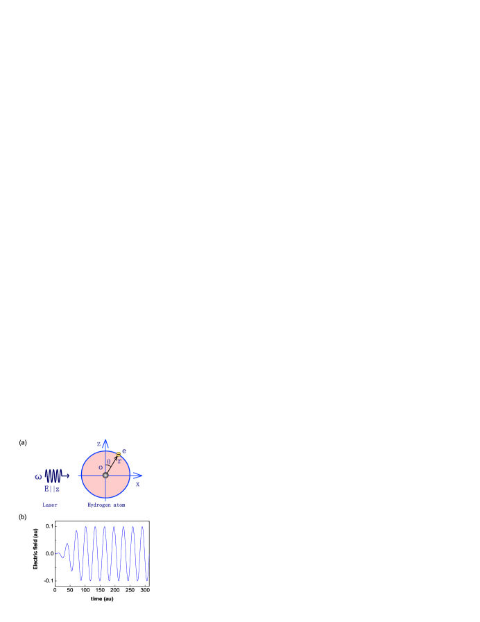
Figure 1: (color online). (a) Graphic description of the direction of the linearly polarized laser field ($\mathbf{E}||\mathbf{z}$) at frequency $\omega$ and the coordinate of the Hydrogen system; (b) Laser field profile in the first ten periods, where the laser period $T=10\pi$ in our work.

The system we consider in this paper is a Hydrogen atom in intense laser field. The Schrödinger equation for the system can be written as (atomic units are used throughout)

$$i\frac{\partial\psi(\mathbf{r},t)}{\partial t}=[H_{0}(\mathbf{r})+H_{I}(\mathbf{r},t)]\psi(\mathbf{r},t).$$ (5)

Here $H_{0}(\mathbf{r})$ is the field-free Hydrogen atom Hamiltonian and $H_{I}(\mathbf{r},t)$ is the intense laser-atom interaction: $H_{0}(\mathbf{r})=-\frac{1}{2}\frac{d^{2}}{dr^{2}}+\frac{\widehat{L}^{2}}{2r^{2}}-\frac{1}{r},H_{I}(\mathbf{r},t)=-\mathbf{r\cdot E}(t)=-zE(t)$, where the laser is the linearly polarized field ($\mathbf{E}||\mathbf{z}$) and $E(t)$ is the laser field profile. Due to the linearly polarized laser field, magnetic quantum number $m$ of the atom is a good quantum number, so that the problem of solving the time-dependent Schrödinger equation here can be simplified into a two-dimensional problem (see figure 1(a)). In our study we use the grid method and the second-order split-operator technique to numerically solve the time-dependent Schrödinger equation (5), which has been detailedly introduced by Tong and Chu tong . The laser field profile is

$$E(t)=\left\{\begin{array}[]{ll}E_{0}\sin^{2}(\frac{\pi t}{6T})\sin(\omega t),&{0\leq t\leq 3T}\\ E_{0}\sin(\omega t),&{\ t>3T,}\end{array}\right.$$ (6)

where $T=2\pi/\omega$, $E_{0}$ and $\omega$ are the electric field amplitude and angular frequency, respectively (see figure 1(b)). Here we take $E_{0}=0.1$ au and $\omega=0.2$ au The initial state $\psi(\mathbf{r},0)$ of the system is in the ground state of the field-free Hydrogen atom.

IV Result

IV.1 Electron trajectory from the Bohm-Newton equation

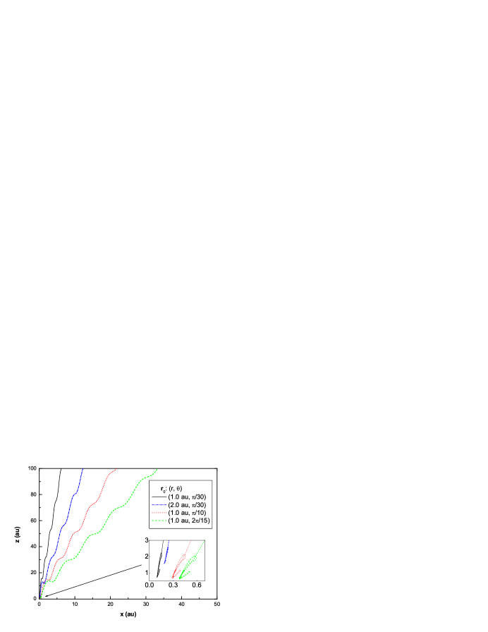
Figure 2: (color online). The electron trajectories in the spatial coordinate with the corresponding initial positions $\mathbf{r}_{0}$. The initial positions $\mathbf{r}_{0}$ in the polar coordinate are from top to bottom: $(1.0$ au$,\pi/30)$, $(2.0$ au$,\pi/30)$, $(1.0$ au$,\pi/10)$, and $(1.0$ au$,2\pi/15)$, respectively.

After numerically obtaining the time-dependent wavefunction $\psi(\mathbf{r},t)$, and then the phase $S(\mathbf{r},t)$, we can get the trajectory of an electron by integrating equation (4) with its initial value of position $\mathbf{r}_{0}$ (see appendix A). In this way, we can gain an ensemble of electron trajectories according to the initial distribution of electrons $\left|\psi(\mathbf{r},0)\right|^{2}$, where $\psi(\mathbf{r},0)$ is the ground state of the field-free Hydrogen atom. Explicitly, we present four trajectories of electron with the corresponding initial positions in figure 2. Let’s take one electron trajectory as an example with $\mathbf{r}_{0}=(1.0$ au, $\pi/30)$ in the polar coordinate. The path of the electron has the following character in the spatial coordinate: The motion is irregular when the electron is near the parent ion; after the electron has been driven far away from the parent ion by the intense laser field, it travels in a straight line with a little oscillation. The reason why the motion of the electron keeps oscillating as the electron is far away from the parent ion is due to the existence of the laser field. The other trajectories with different initial positions have similar character as shown in figure 2.

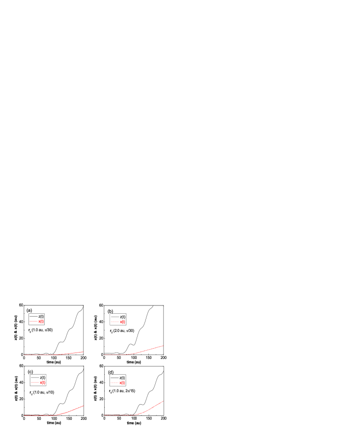
Figure 3: (color online). Projections of electron trajectories in $z$ and $x$ directions as functions of time. The corresponding initial positions of electrons are, from (a) to (d), $(1.0$ au$,\pi/30)$, $(2.0$ au$,\pi/30)$, $(1.0$ au$,\pi/10)$, and $(1.0$ au$,2\pi/15)$, respectively. It is obvious that the motion of the electron in $x$ direction is uniform while its motion in $z$ direction has undulations as the electron is far from the core. The reason for the $z$-undulation is due to the existence of laser field ($\mathbf{E||z}$).

In figure 3, we show the projections of electron trajectory in $z$ and $x$ directions, respectively, as functions of time. In figure 3(a), two curves $z(t)$ and $x(t)$ are obtained from the electron trajectory with $\mathbf{r}_{0}=(1.0$ au, $\pi/30)$. At the beginning, both $z(t)$ and $x(t)$ are near the core. After the time $t\approx 130$ au, $z(t)$ becomes a regular wave curve and $x(t)$ seems to be a straight line. Similarly, we have obtained the projections of three other electron trajectories with their initial positions $\mathbf{r}_{0}$ (see figures 3(b)-(d)). All of them have the similar character as that in figure 3(a).

IV.2 Time-dependent quantum potential in intense laser-atom physics

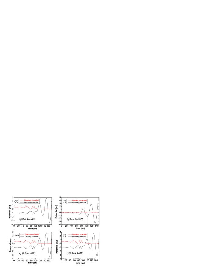
Figure 4: (color online). The time-dependent value of quantum potential and ordinary potential of the electrons with the corresponding initial positions, $(1.0$ au$,\pi/30)$, $(2.0$ au$,\pi/30)$, $(1.0$ au$,\pi/10)$, and $(1.0$ au$,2\pi/15)$, respectively.

In Section II, we have discussed that quantum potential $Q(\mathbf{r},t)$ together with ordinary potential $V(\mathbf{r},t)$ dominates the motion of particle in BM. And quantum potential plays a crucial role for the appearance of quantum phenomenon. If the value of $Q(\mathbf{r},t)$ smoothly trends to be negligible ($Q\rightarrow 0$), equation (3) will reduce to Newton equation and then the motion of electron can be described by classical mechanics.

Now we study the change of quantum potential for an atomic electron as it is driven away by the laser field. After obtaining the time-dependent wavefunction $\psi(\mathbf{r},t)$ and the electron trajectories $\mathbf{r}(t)$, we calculate the changes of quantum potential $Q(\mathbf{r}(t))$ (see appendix B). In figure 4, we show the time-dependent values of quantum potential $Q(\mathbf{r}(t))$ and ordinary potential $V(\mathbf{r}(t))=-\frac{1}{r}-zE(t)$ with the corresponding initial positions $\mathbf{r}_{0}$. Here we take the electron with $\mathbf{r}_{0}=(1.0$ au, $\pi/30)$ as an example (see figure 4(a)). The value of quantum potential is comparable with that of ordinary potential in the early period. After some time, e.g., after 100 au about, quantum potential smoothly becomes smaller and then it trends to be negligible, particularly after the time $t\approx 133$ au The changes of quantum potential of three other electrons are presented in figures 4(b)-(d), and they have the similar character as that in figure 4(a). In this way, our numerical results present an explicit picture of the reduction from the Bohm-Newton equation to Newton equation. Consequently, the Bohmian trajectory method can give both the quantum and classical descriptions of the motion of an atomic electron in intense laser-atom physics.

IV.3 Classical description after the electron has been ionized

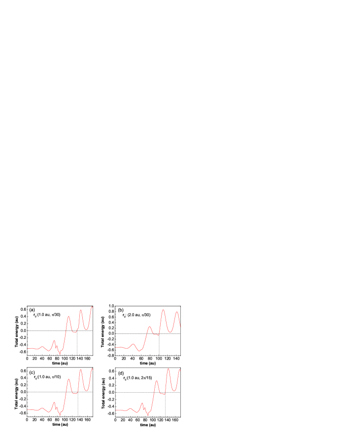
Figure 5: The time-dependent total energies of an electron (including kinetic energy, Coulomb potential and quantum potential) with the initial positions, $(1.0$ au$,\pi/30)$, $(2.0$ au$,\pi/30)$, $(1.0$ au$,\pi/10)$, and $(1.0$ au$,2\pi/15)$, respectively.

As we have shown above, the Bohm-Newton equation of electron is approaching to Newton equation in intense laser-atom physics, as the electron was driven far away from the parent ion. In the previous semiclassical approaches of intense laser-atom physics, the ionized electron motion is usually treated by the classical dynamics, while quantum mechanics is used before the ionization Corkum ; Corkum2 ; Schafer ; Paulus ; Salieres . Here, we want to verify whether the motion of an electron can be treated by classical dynamics or not, i.e. whether the quantum potential becomes negligible or not, as it has been ionized.

In figure 5, we show the total energies of an electron (including kinetic energy, Coulomb potential and quantum potential) with different initial positions. When the total energy becomes positive, the electron will be ionized. Here we take the electron with $\mathbf{r}_{0}=(1.0$ au, $\pi/30)$ as an example (see figure 5(a)). At the beginning, the value of the total energy is less than zero, i.e. the electron is bounded by the core. After the time $t\approx 103$ au, the total energy becomes positive but it then turns to the negative at the time $t\approx 120$ au The reason why the total energy of the ionized electron turns to the negative again may be that the electron with low energy is not far enough from the core and it is recaptured by the parent ion with a photon emitted when the laser field reverses. The total energy becomes positive again and higher than before at $t\approx 133$ au and thereafter, i.e. the electron can never be recaptured again by the parent ion. On the other hand, in figure 4(a), we found the value of quantum potential of the electron trends to be trivial soon after the time $t\approx 133$ au (The corresponding distance between the ionized electron and the core is 16.2 au about; see figure 3). Similarly, in figures 5(b)-(d) and 4(b)-(d), we can find when the electron is ionized, the corresponding quantum potential trends to be negligible. Therefore, our numerical solutions show that the quantum potential is negligible as the ionized electron was driven far away from the core and thus the motion of ionized electron is dominated by classical mechanics. In this way, our work may present a direct positive evidence for the semi-empirical assumption in the semiclassical approaches of intense laser-atom physics, such as the three-step model Corkum and Feynman’s path-integral approach in the strong field approximation Salieres , in which the motion of ionized electrons is treated by classical dynamics directly. Furthermore, the Bohmian trajectory method can help us to find how far the electron from the core when it was ionized, while the initial position of an ionized electron is assumed to be 0 in the semiclassical approaches Corkum .

V Discussion

As it has been discussed above, quantum potential dominates the quantum behavior of a physical system. In the prior work of quasistatic model of strong-field multiphoton ionization Corkum , a dual procedure was considered to describe the multiphoton phenomena in intense laser-field physics. First a tunneling model is applied to obtain the ionization rate and describe the formation of a sequence of wave packets. The second part of the quasistatic procedure uses the classical mechanics to describe the evolution of an electron wave packet. It has been pointed out definitely that only the Newton equation cannot give the ionization rate correctly, unless a quantum tunneling process was allowed jsc . This is consistent with our numerical results in this paper: The quantum potential cannot be ignored before the ionization, i.e. quantum mechanics is needed to study the behavior of the electron before the ionization, but the motion of an ionized electron can be described by classical mechanics directly .

VI Remark

It is interesting that Mahmoudi et al mah have studied free-electron quantum signatures in intense laser fields by looking for negativities in the Winger distribution. They concluded that the quantum signatures of the free electron get washed away, provided the dipole approximation is made. In this way, their work presents another evidence for the treatment of ionized electron in the semiclassical approaches of intense laser-atom physics.

VII Acknowledgement

We thank J. B. Delos and L. You for helpful discussions. This work is supported by National Basic Research Program of China under Grant No. 2006CB921203.

Appendix A Electron quantum trajectory

In this appendix, we show how to obtain the electron quantum trajectory from equation (4). First, equation (4) can be expressed as (atomic units are used)

$$\frac{d\mathbf{r}}{dt}=\nabla S(\mathbf{r},t)=\text{Im}\frac{\nabla\psi(\mathbf{r},t)}{\psi(\mathbf{r},t)},$$ (7)

where $\psi(\mathbf{r},t)=R(\mathbf{r},t)e^{iS(\mathbf{r},t)}$ and $\text{Im}(f)$ is the imaginary part of $f$. In our study $\psi(\mathbf{r},t)$ is gained by numerically solving the time-dependent Schrödinger equation (5), using the grid method and the second-order split-operator technique, which has been detailedly introduced by Tong and Chu tong . Then we use the Runge-Kutta method to evolve equation (7) to obtain the electron quantum trajectory.

In our numerical procedure, the range of the variable $\mathbf{r}$ in the radial direction is confined to $(0,150$ au$)$. In the grid method, the numbers of grid points are $350$ in the $r$ direction and $51$ in the $\theta$ direction. The time step for the evolution is $0.01$ au

Appendix B Time-dependent value of quantum potential

After obtaining the time-dependent wavefunction $\psi(\mathbf{r},t)$ and the electron quantum trajectory $\mathbf{r}(t)$ with the corresponding initial position $\mathbf{r}_{0}$, we can numerically obtain the value of the quantum potential $Q(\mathbf{r}(t))$ along the trajectory $\mathbf{r}(t)$. First, the quantum potential $Q(\mathbf{r},t)$ can be written as

$$Q(\mathbf{r},t)=-\frac{1}{2}\frac{\nabla^{2}R(\mathbf{r},t)}{R(\mathbf{r},t)}=-\frac{1}{2}\left[\text{Re}\frac{\nabla^{2}\psi(\mathbf{r},t)}{\psi(\mathbf{r},t)}+\left(\text{Im}\frac{\nabla\psi(\mathbf{r},t)}{\psi(\mathbf{r},t)}\right)^{2}\right],$$ (8)

where $\text{Re}(f)$ is the real part of $f$. Secondly, inserting the quantum trajectory $\mathbf{r}(t)$ into equation (8), we can numerically get the value of quantum potential $Q(\mathbf{r}(t))$.

References

- (1) Burnett K, Reed V C and Knight P L 1993 J. Phys. B 26 561
- (2) Corkum P B 1993 Phys. Rev. Lett. 71 1994
- (3) Corkum P B, Burnett N H and Brunel F 1989 Phys. Rev. Lett. 62 1259
- (4) Schafer K J et al 1993 Phys. Rev. Lett. 70 1599
- (5) Paulus G G et al 1994 J. Phys. B 27 L703
- (6) Lewenstein M, Balcou Ph, Ivanov M Yu, L’Huillier Anne and Corkum P B 1994 Phys. Rev. A 49 2117
- (7) Bohm D 1952 Phys. Rev. 85 16; Bohm D 1952 Phys. Rev. 85 180
- (8) Holland P R 1993 The Quantum Theory of Motion (England: Cambridge University Press, Cambridge)
- (9) Nikolic H 2008 Am. J. Phys. 76 143
- (10) Wyatt R E 2005 Quantum Dynamics with Trajectories: Introduction to Quantum Hydrodynamic (New York: Springer); Lopreore C L and Wyatt R E 1999 Phys. Rev. Lett. 82 5190
- (11) Philippidis C, Dewdney C and Hiley B 1979 Nuovo Cimento 52B 15
- (12) Hirschfelder J O, Christoph A C and Palke W E 1975 J. Chem. Phys. 61 5435
- (13) Dewdney C and Hiley B J 1982 Found. Phys. 12 27
- (14) Oriols X 2007 Phys. Rev. Lett. 98 066803
- (15) Sanz A S, Borondo F and Miret-Artés S 2000 Phys. Rev. B 61 7743
- (16) Makowski A J and Górska K J 2002 Phys. Rev. A 66 062103; Makowski A J 2002 Phys. Rev. A 65 032103
- (17) Makowski A J 2003 Phys. Rev. A 68 022102
- (18) Rosen N 1964 Am. J. Phys. 32 377
- (19) Schwengelbeck U and Faisal F H M 1995 Phys. Lett. A 199 281; Schwengelbeck U and Faisal F H M 1995 Phys. Lett. A 207 31
- (20) Efthymiopoulos C and Contopoulos G 2006 J. Phys. A 39 1819
- (21) Lai X Y, Cai Q Y and Zhan M S 2009 Eur. Phys. J. D 53 393
- (22) Lai X Y, Cai Q Y and Zhan M S 2009 Chin. Phys. B (in press); arXiv: 0911.1529 (atom-ph)
- (23) Tong X M and Chu S I 1997 Chem. Phys. 217 119
- (24) Salieres P et al 2001 Science 292 902
- (25) Cohen J S 2001 Phys. Rev. A 64 043412; Recently, one work also conclued that the classical trajectory method should be improved further by including nonclassical effects (see Botheron P and Pons B 2009 Phys. Rev. A 80 023402)
- (26) Mahmoudi M, Salamin Y I and Keitel C H 2005 Phys. Rev. A 72 033402