Study of sdO models: mode trapping

Abstract

We present the first description of mode trapping for sdO models. Mode trapping of gravity modes caused by the He/H chemical transition is found for a particular model, providing a selection effect for high radial order trapped modes. Low- and intermediate-radial order p-modes (mixed modes with a majority of nodes in the P-mode region) are found to be trapped by the C-O/He transition, but with no significant effects on the driving. This region seems to have also a subtle effect on the trapping of low radial order g-modes (mixed modes with a majority of nodes in the G-mode region), but again with no effect on the driving. We found that for mode trapping to have an influence on the driving of sdO modes (1) the mode should be trapped in a way that the amplitude of the eigenfunctions is lower in a damping region and (2) in this damping region significant energy interchange has to be produced.

1 Introduction

Subdwarf O (sdO) stars cover a domain of approximately 60 000 K in $T_{\mathrm{eff}}$ and 2.5 dex in $\log g$ in the hot and high gravity domain of the HR diagram. Due to the wide spread of physical parameters their evolutionary stage is not completely understood, but some progress has recently been made with larger than ever (comprising up to a hundred sdOs) spectroscopic studies (Ströer et al. 2007; Hirsch & Heber 2008). Determinations of $T_{\mathrm{eff}}$, $\log g$ and helium abundance allowed Ströer et al. (2007) to make some statistical correlations between position in the HR and evolutionary stage, and as a result they propose that sdOs come from a mixed population of post-EHB (i.e. sdB descendants), post-AGB and post-RGB objects. The canonical picture depicts them as objects of about half a solar mass with an inert carbon-oxygen core, and helium and hydrogen burning layers.

Table 1: Main physical parameters and mass fractions of the sdO model used. X(other) refers to the mass fractions of all the other elements. Z is the initial and current metallicity of the model.

$T_{\mathrm{eff}}$	$\log g$	M	$\eta_{\mathrm{R}}$	X(H)	X(He3)	X(He4)	X(C)	X(N)	X(O)	X(other)	Z
(K)		(M⊙)
45 000	5.26	0.469	0.650	0.59	1.2E-03	0.35	7.4E-03	4.2E-03	2.4E-02	1.5E-02	0.05

A milestone for sdOs was passed in 2006 with the discovery of the first, and unique to date, pulsating sdO SDSS J160043.6+074802.9 (known in short as J1600+0748) by Woudt et al. (2006). This object is a very fast pulsator, with a main period of $\sim$120 s, and at least seven other frequencies (Rodríguez-López et al., 2009a) between the main frequency and its first harmonic. The excited frequencies were identified by Fontaine et al. (2008) as p-modes and its pulsations explained as a classical $\kappa$ mechanism with the aid of appropriate models including radiative levitation of iron. Our own attempts of exciting p-mode pulsations in uniform metallicity sdO models failed (Rodríguez-López et al. 2009b, Paper I), although some models, as this one, were found to present a certain tendency to instability in the p-mode region. During the course of our investigation of pulsational properties of sdO models, for which g-mode driving was found, a particular model presenting g-mode trapping was discovered.

In main sequence stars the asteroseismic potential of g-mode trapping to study the mixing processes within the convective core and their effects on the surrounding chemical gradient have been well documented by Miglio et al. (2008). In the case of compact pulsators, g-mode trapping has been described extensively for sdBs (Charpinet et al., 2000), DA and DB white dwarfs, and GW Vir pre-white dwarfs (see e.g. Winget, Van Horn & Hansen 1981; Brassard et al. 1991; Brassard et al. 1992, or more recently Córsico & Althaus 2006; Gautschy & Althaus 2002) as due to chemical stratification in the envelope of these stars. Because gravity modes are trapped in the outer envelope, they have lower amplitude in the damping core, which intensifies their instability. This may help, in some cases, alleviate the problem of observing less modes than predicted by the models. It also provides a useful tool to determine the mass and width of the surface layer (see e.g. Brassard et al. 1992; Kawaler & Bradley 1994). Charpinet et al. (2000) reported gravity mode trapping due to the transition between the helium core and the hydrogen-rich envelope in sdB models. They also identified subtle, but non-negligible departures from uniform frequency spacing for pressure modes, caused by the same chemical transition region.

In sdB models, the maximum gradient in Brunt-Väisälä (BV) frequency is produced at the transition of the helium radiative core to the hydrogen envelope. In sdO models the BV profile is more complex, since as evolution proceeds, a C-O core builds up, resulting in two chemical transitions: one from the C-O core to the He burning shell, and another one from the He radiative shell to a H burning shell. This renders the mode trapping effects more complex in sdO than in sdB models.

We report in this study the discovery of g-mode trapping in a sdO model caused by the He/H transition. This provides a selection mechanism in the way that trapped modes would be more easily excited. Low- and intermediate radial order p-modes are found to be trapped by the deeper transition from the C-O/He, but with no significant effects on the driving.

The importance of g-mode trapping is evident as a way to probe the deep stellar interior, where gravity modes propagate, unattainable in any other way; but also to derive information about the location and width of the chemical transitions and the mass of the envelope.

The paper is organized as follows: in Section 2 we describe some general characteristics of the sdO model used. In Section 3 we describe the g-mode trapping and the effects of cancelling out the He/H and C-O/He chemical transitions in BV frequency on the trapping and driving of the modes. Section 4 does a similar treatment for p-modes. Finally, Section 5 presents a summary and Section 6 the discussion and conclusions.

2 The Model

This theoretical exercise arose as an exploration of a particular sdO model, whose properties were thoroughly described in Paper I and parameters given in Table 1. The model, built with JMSTAR code (Lawlor & MacDonald, 2006), comes from a 1 M$\odot$ star on the pre-main sequence with enhanced mass loss rate on the red giant branch, that drives the star to evolve to higher temperatures at constant luminosity. A delayed helium-flash puts the star back in the horizontal branch, and further evolution brings the star to the sdO domain. The sdO models have developed a carbon-oxygen core while helium and hydrogen shell burning is still produced (Fig. 1 left). The change in chemical composition from the C-O core to the He burning shell, and from the He radiative layer to the H burning shell is seen in the two steep peaks in BV frequency and subtler transitions in Lamb frequency (Fig. 1 right).

Figure 1: Left: Normalised nuclear energy generation rate as a function of the fractional mass depth parameter ($\log q=1-M_{r}/M_{T}$). The deeper peak at $\log q\simeq-0.8$ corresponds to the helium burning shell; the shallower peak at $\log q\simeq-2.2$ to the hydrogen burning shell. Right: Brunt-Väisälä frequency (solid line) showing the two peaks corresponding to the maximum chemical gradients: from the C-O core to the He burning shell ($\log q\simeq-0.8$), and from the He radiative shell to hydrogen shell burning ($\log q\simeq-2.2$). Lamb frequency (dashed line) for $\ell=2$ modes is also shown.

The model, which was subject to a non adiabatic analysis with GRACO (Moya et al. 2004; Moya & Garrido 2008), was found stable in the frequency range $\sim$0.5 to 25 mHz. However, an oscillatory behaviour of the growth rate at low and intermediate frequencies (see fig. 10 of Paper I) caught our attention. That drove us to explore the behaviour of the kinetic energy of the modes, which revealed that the model experienced mode trapping effects.

3 Gravity modes

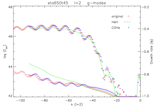
Figure 2: Logarithm of the total kinetic energy vs. radial order for g-modes (this and subsequent plots have been made for $\ell=2$ modes) of the original (upper circles) and perturbed models without the He/H (upper solid line) and C-O/He (upper crosses) transition regions. Lower symbols plot the corresponding growth rates whose values can be read on the right axis.

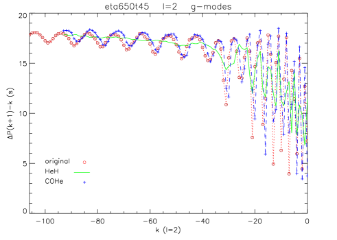
Figure 3: Period spacing for g-modes with the same degree $\ell$ and consecutive radial orders for the original (circles and dotted line) and perturbed He/H (solid line) and C-O/He (crosses and dashed line) models.

The logarithm of the total kinetic energy of each g-mode and its growth rate $\eta$ are given in Fig. 2 (upper and lower circles, respectively, the meaning of the other symbols will be explained below). The plot reveals that in the region of very high-radial order g-modes (radial order $k\gtrsim 40$), there are small variations in the kinetic energy, of no more than one order of magnitude, between different modes. We also see that modes with local minimum values of the kinetic energy have local maximum growth rates and vice versa.

The non-uniform distribution of the kinetic energy resembles the mode trapping phenomenon caused by the potential barrier due to the composition transition regions. The chemical transition regions act as resonant cavities for the modes, changing the amplitudes of the eigenfunctions in different regions of the star and hence modifying their kinetic energy, which is given by:

$$E_{kin}=\frac{1}{2}\sigma^{2}\int_{0}^{R}\left(|\xi_{r}|^{2}+l\left(l+1\right)|\xi_{h}|^{2}\right)4\pi\rho r^{2}dr$$ (1)

where $\sigma$ is the eigenfrequency, $\xi_{r}$ and $\xi_{h}$ the radial and horizontal displacement eigenfunctions, and $\rho$ the local density. It follows that g-modes will have higher kinetic energies than p-modes, as they propagate in denser regions of the star. This is clearly seen by comparing Fig. 2 and the corresponding plot for p-modes, Fig. 10.

Following the asymptotic theory of nonradial oscillations (see e.g. Tassoul, 1980; Smeyers et al., 1995; Smeyers & Moya, 2007), modes of the same degree $\ell$ and consecutive radial order $k$ would have a uniform period separation, $\Delta P$, given by:

$$\Delta P=P_{k+1,l}-P_{k,l}=2\pi^{2}\left[\int_{0}^{R}\frac{|N|}{r}dr\right]^{-1}\left[l\left(l+1\right)\right]^{-\frac{1}{2}}$$ (2)

where $N$ is the BV frequency. Thus, mode trapping effects are revealed for certain modes as deviations with respect to the mean period spacing. This can be seen from the data points plotted in red in Fig. 3.

The radial and horizontal displacement eigenfunctions (y${}_{1}=\xi_{r}/r$ and y${}_{2}=(\sigma^{2}r/g)*\xi_{h}/r$, respectively as defined by Dziembowski 1971) of representative modes with minimum (g88), normal (g85) and maximum (g83) total kinetic energy are shown in Fig. 4. The vertical line at $\log q\simeq-2.23$ marks the location of the maximum composition gradient in the He/H transition region. It is evident that the g88 mode has lower amplitude below the He/H interface, so it is trapped in the envelope. As the region below the He/H transition is very dense, it has a high weight in the total kinetic energy, and hence trapped modes have minimum values of the kinetic energy. We recall that, for high-radial order g-modes in this model, significant energy interchange is produced in the region below the He/H transition, which is mostly damping (fig. 8, Paper I), resulting in trapped modes being less damped and having maximum growth rate values. On the other hand, the g83 mode has highest amplitude in the damping region, and it is referred to as a confined mode, which is less likely to be excited, as is reflected in its minimum value of the growth rate.

Previous adiabatic studies for sdBs (Charpinet et al., 2000) postulated qualitatively, based on the growth rate dependence of the kinetic energy, $\eta\,\alpha\,W/E_{kin}$ (where $W$ is the work integral defined as the total energy balance over one period of oscillation), that when a mode had lower amplitude in the damping regions, the mode would be less damped and would be more likely to be excited. Indeed, we confirm this hypothesis for high-radial order sdO gravity modes in our non-adiabatic study.

Figure 4: Radial (left) and horizontal (right) displacement eigenfunctions for trapped (g88), normal (g85) and confined (g83) g-modes of the original model. The vertical line marks the location of the He/H transition. The insets show a blow-up of this region.

Figure 5: Weight function for g88, g85 and g83, a trapped, normal and confined mode, respectively for the original model (left) and modes with equivalent frequencies for the model without He/H chemical transition (right). Inset showing a blow-up of the He/H transition region.

We also draw the attention to the fact that the radial eigenfunction for the trapped mode has a node above the He/H transition, while the confined mode has a node below it, and  the normal mode has a node just about on the interface. For the horizontal eigenfunction, although there are nodes at similar distances above and below the He/H transition, for the trapped (confined) mode, the closest node to the transition is below (above) it, in good agreement which what is found for sdBs and white dwarfs. However, the larger distances of the nodes to the trapping region in our model translate into less efficiency of the trapping/confinement mechanism.

In our model, the smaller differences in the kinetic energy between trapped and confined modes comparing to sdB or white dwarf modes, are due to the fact that the mode trapping interface (the He/H transition, see below) is located much deeper in the envelope ($\log q\sim-2$) than for sdBs ($\log q\sim-4$, in Charpinet et al. 2000) or white dwarfs ($\log q\sim-10$, in Brassard et al. 1992). As a result, both the trapped and confined region, weighted by the density, $\rho$ (see Eq. 1), contribute largely to the kinetic energy.

Also from Charpinet et al. (2000) and Brassard et al. (1992), trapped modes in sdBs and white dwarfs have sharp kinetic energy minima, while maxima, corresponding to confined modes, are somewhat wider, comprising up to three modes and indicating that confinement processes are not so effective as mode trapping. In our model, both the minima and the maxima in the kinetic energy have a certain width, revealing that both the mode trapping and confinement processes are not so sharp as in sdBs and white dwarfs. The explanation lies in the wider chemical transition regions in the sdO model (see Fig. 1, right) in comparison to those for sdBs and white dwarfs (see e.g. fig. 3 of Charpinet et al. 2000 and fig. 1 of Brassard et al. 1992).

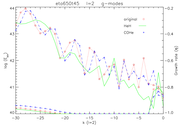
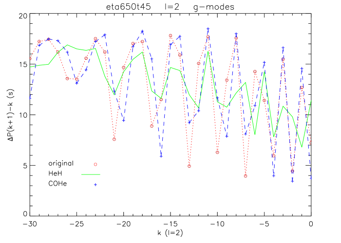
Figure 6: Left: Logarithm of the kinetic energy vs. radial order for low-radial order g-modes of the original (upper circles and dotted line) and perturbed models without the He/H (upper solid line) and C-O/He (upper crosses and dashed line) transition regions. Lower symbols plot the corresponding growth rates whose values can be read on the right axis. Right: Period spacing for low-radial order g-modes with the same degree $\ell$ and consecutive radial orders for the original and perturbed He/H and C-O/He models (with same symbols as in the left pannel).

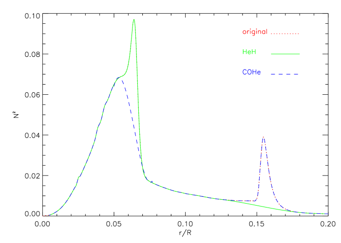
Figure 7: Original (dotted) Brunt-Väisälä frequency (left) and sound speed (right) and modifications cancelling out the He/H (solid) and sharp peak of the C-O/He (dashed) chemical transition regions.

A clearer view of the local contribution of each region of the star to the formation of a particular mode is given through the so-called weight function, defined in Charpinet et al. (2000) as:

$$F\left(\xi_{r},P^{\prime},\Phi^{\prime};r\right)=\left[\xi_{r}^{2}N^{2}+\frac{(P^{\prime})^{2}}{\Gamma_{1}P\rho}+\left(\frac{P^{\prime}}{\Gamma_{1}P}+\xi_{r}\frac{N^{2}}{g}\right)\right]\rho r^{2}$$ (3)

where $P^{\prime}$ and $\Phi^{\prime}$ are the Eulerian perturbations of the pressure and potential, respectively and $\Gamma_{1}$ is an adiabatic exponent.

A plot of the weight function for the same trapped (g88), normal (g85) and confined mode (g83) (Fig. 5 left), each of them normalised individually, shows that the wide C-O/He chemical transition region has an important contribution for all of them, as expected for high-radial order g-modes, which mainly propagate in the deep interior of the star. The main difference in the weight function for the different modes is the higher contribution of the He/H transition region to the formation of the trapped mode, which also has a higher contribution of the outer zones. This becomes even clearer when we eliminate in the model the He/H chemical transition region (Fig. 5 right, explanation below).

A blow up of Fig. 2 for the low-radial order g-modes ($k$ up to 30) is shown in the left panel of Fig. 6 (circles and dotted lines), and the period differences in this zone in the right panel. We still notice the existence of certain modes alternating maximum and minimum values of the kinetic energy, until about $k=10$. The period differences between modes also show deviations with respect to the mean value, a signature of mode trapping. However, contrary to high-radial order g-modes, this trapping/confinement phenomenon, does not have any influence on the ability to excite the modes, as they remain highly stable. This is explained as, for g-modes of low-radial order, the energy interchanged below the He/H transition is negligible compared to the energy interchanged at the Z-bump region, located at $-10.0\lesssim\log q\lesssim-9.5$. There, the energy contribution for both trapped and confined modes is always damping (see fig. 8 in Paper I). So, even if the mechanical effect of the mode trapping is maintained, at the frequencies in which low-radial order g-modes occur, the significant energy interchange is produced in different regions of the star, therefore the trapping has no influence in the growth rate.

3.1 Perturbation analysis

We have investigated the effects of cancelling out the He/H and the sharp peak of the C-O/He chemical transition regions of the Brunt-Väisälä frequency and sound speed (Fig. 7) in this sdO model on mode trapping and the tendency of modes to instability. To do this, we described the perturbation of the mass, pressure, sound speed squared ($c^{2}$) and BV squared ($N^{2}$) as a function of the perturbation of the density, gravity and adiabatic exponent. From these relations we derived an expression for the perturbation of the density as a function of the perturbations introduced for BV and the sound speed ($\delta N^{2},\delta c^{2}$). Finally, we wrote the perturbation of the dynamical variables of the model as a function of the already calculated perturbations (a complete description of the mathematical formulation is given in Appendix A). These new perturbed models underwent again the non-adiabatic analysis.

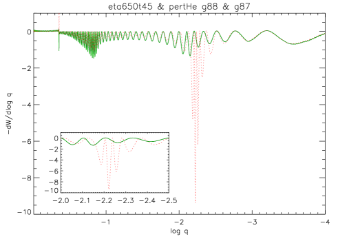
Figure 8: Differential work for g88 mode of the original (dotted) model and g87 mode of the pertHeH (solid) model. The inset zooms in on the He/H chemical transition. See text for details.

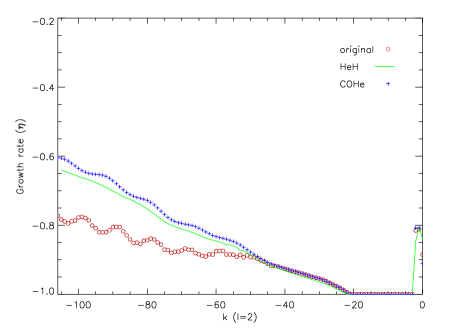
Figure 9: Growth rates of the original model (circles), the same model with the differential work integrated only over $\log q\leq-2.24$ (crosses) and the pertHeH model (solid line).

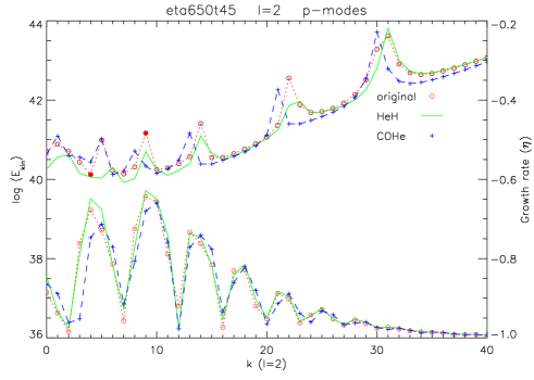
Figure 10: Logarithm of the total kinetic energy vs. radial order for p-modes of the original (upper circle and dotted line) and perturbed models without the He/H (upper solid line) and C-O/He (upper crosses and dashed line) transition regions. Lower symbols plot the corresponding growth rates whose values can be read on the right axis. Filled circles mark p4 and p9 modes showing maximum growth rate values. See Section 5 for more details.

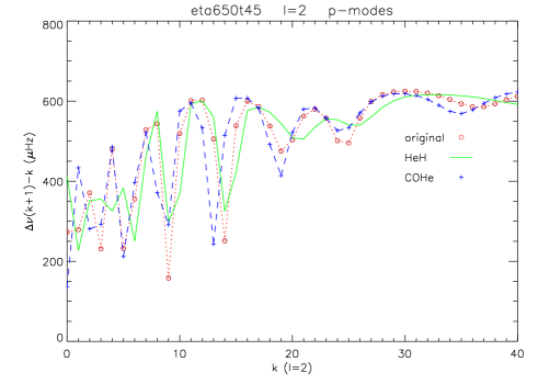
Figure 11: Large frequency spacing vs. radial order for p-modes with the same degree $\ell$ and consecutive radial orders for the original, and perturbed models.

3.1.1 Cancelling out the He/H transition

When we cancel out the He/H chemical transition region, we get a smooth kinetic energy for all the modes (Fig. 2, upper solid line). Trapped modes vanish, revealing that the He/H transition is the main factor responsible for their occurrence. The plot of the weight function (Fig. 5, right) reveals that the He/H region, once cancelled, no longer has any significant influence on mode formation. We also note that the growth rate no longer oscillates with frequency (Fig. 2, lower solid line), as expected from the uniform kinetic energy; and we also get a uniform period separation (Fig. 3, solid line). However, perturbed modes equivalent to trapped modes in the original model achieved higher values of the growth rate, while their kinetic energy was higher, which seems to be at odds with the growth rate dependence on the kinetic energy.

The local minimum in the damping energy for model 8 at $\log q=-2.23$ (Fig. 8, dotted line), which is absent in model pertHeH (Fig. 8, solid line), is responsible for the overall lower values of the growth rate in the original model. Thus, when we calculate the work function for the original model integrating between $\log q\leq-2.24$ and the surface, we obtain similar growth rate values as those of the pertHeH model (Fig. 9).

In the case of low radial order g-modes (Fig. 6, solid lines) some subtle mode trapping seems still to be present. This may be due to remnant mode trapping effects caused by the C-O/He transition, in the same way as described below for low radial order p-modes.

Figure 12: Radial (left) and horizontal (right) displacement eigenfunctions for a trapped, normal and confined p-mode of the original model:p9, p8 and p7, respectively. Dashed-dotted vertical lines delimit the convective region where maximum opacity takes place. Dashed vertical lines in the insets mark the maxima of the C-O/He (the deepest) and He/H transition regions.

3.1.2 Cancelling out the C-O/He transition

When we cancel out the sharp peak of the C-O/He chemical transition, keeping the He/H peak, we still obtain the original pattern of trapped modes, with total kinetic energy, growth rate and period differences similar to those of the original model (Fig. 2, Fig. 3 crosses and dashed lines). Thus, this chemical transition plays no role in high radial order g-mode trapping. However, for lower order modes (Fig. 6, left panel, crosses and dashed lines), it may have some influence, which is revealed in certain alterations to the total kinetic energy of each mode.

4 Pressure modes

The logarithm of the total kinetic energy, and corresponding growth rates, for the p-mode spectrum are shown in Fig. 10. The depicted radial orders correspond to frequencies ranging from about 6 to 25 mHz. There are certain modes which show values higher than the mean kinetic energy in the original and perturbed models. We investigate if this could also be an effect of mode trapping.

Following again the asymptotic theory of nonradial oscillations (Tassoul, 1980; Smeyers et al., 1995; Smeyers & Moya, 2007) p-modes of the same degree $\ell$ and consecutive radial order $k$, will have constant frequency separation, $\Delta\nu$, given by :

$$\Delta\nu=\nu_{k+1,l}-\nu_{k,l}=\frac{1}{2}\left[\int_{0}^{R}\left(\frac{\rho}{\Gamma_{1}p}\right)^{1/2}dr\right]^{-1}$$ (4)

Thus, the mode trapping signature for p-modes would show up in the deviations in the large frequency spacing for the original and the perturbed He/H model (Fig. 11).

Figure 13: Left: Local kinetic energy for trapped, normal and confined modes: p9, p8, p7, respectively. Right: Differential work and opacity (long dashed line) for the same modes. The maximum of the Z-bump is located at $\log q\simeq-9.5$.

We have plotted the radial and horizontal displacement eigenfunctions for the original model p-modes with maximum (p9), intermediate (p8) and minimum (p7) total kinetic energy (Fig. 12). We found that all modes show higher amplitude in the envelope, as expected for p-modes. We found that the p9 mode shows the highest amplitude in the outer envelope for the 3 modes under comparison. However, ultimately what accounts for the higher total kinetic energy is the higher amplitude of the eigenfunctions in the innermost layers of the star, where the mode is trapped due to the pinching effect of the C-O/He interface on the eigenfunctions. This can be seen in Fig. 13 (left) that shows the local contribution to the kinetic energy of the trapped, normal and confined modes, p9, p8, p7, respectively, normalised to the maximum of p7. Although not shown for the sake of clarity, the maximum kinetic energy value for the p9 trapped mode reaches one order of magnitude higher.

The plot of the differential work for a trapped, normal and confined mode (Fig. 13, right) shows that significant energy interchange is only produced at the Z-bump; and there, driving is higher for the trapped mode. As it is the case for low-radial order g-modes, a maximum in kinetic energy does not translate into a minimum growth rate value for the mode. This is explained by the maximum kinetic energy being due to a higher amplitude of the eigenfunctions in the region $\log q\gtrsim-0.8$, which for p-modes does not have significant influence on driving. Neither do the higher amplitudes of the eigenfunctions of the trapped mode at the driving region lead to a maximum growth rate value, as consecutive higher radial order modes have even higher amplitudes. We conclude that the influence of the work function prevails over the influence of the kinetic energy in the computation of the growth rate.

Pressure modes with higher radial orders, not shown in Fig. 10, display kinetic energy monotonically increasing, an effect of the nodes accumulating in the surface limit imposed by the boundary conditions, as it is well described in Charpinet et al. (2000). The trapping effect caused by the C-O/He transition is no longer produced, as is expected for high-radial order pure p-modes propagating only in the external layers of the star.

4.1 Perturbation analysis

When we cancel the He/H, or the sharp peak of the C-O/He chemical transitions in the Brunt-Väisälä frequency, and also the corresponding bumps in the sound speed at these locations, we still find a kinetic energy pattern, and an oscillating profile of the growth rate, both similar to those of the original model (Fig. 10, solid and dashed lines, respectively). Therefore, neither the He/H, nor the C-O/He chemical transition, nor the sound speed at these locations, seem to have any significant influence on the kinetic energy or on the tendency to driving of the p-modes.

This result was the expected for the growth rate, for reasons given above, but not for the kinetic energy, as we presumed the modification of the C-O/He transition would show in the kinetic energy profile, due to changes in the amplitude of the eigenfunctions. However, eigenfunction profiles similar to those of Fig. 12 are retained for trapped, normal and confined modes of the perturbed models. The reason may be due to that, in fact, the C-O/He transition still exists (see Fig. 7, left) as we only cancelled out its steep peak, giving a softer profile.

5 Summary

We conclude for the g-mode spectrum that:

• High-radial order g-modes are trapped in the envelope due to the He/H chemical transition. This provides a weak selection mechanism, in the way that trapped modes oscillate with lower amplitudes in the innermost damping region. Thus, trapped modes show lower total kinetic energy and higher values of the growth rate.

• Low to intermediate radial order g-modes (mixed modes) are also trapped in the envelope by the He/H transition. However, this has no significant effects on the driving, as the innermost damping region, at the frequencies at which low g-modes occur, has no significant weight in the energy interchanged by the mode with its surroundings.

• Cancelling out the He/H transition region cancels the mode trapping effects of high order gravity modes, and the growth rate loses its oscillatory behaviour with frequency, as expected. However, modes with local maxima in the kinetic energy and similar interchanged energy at the driving region than their non-perturbed counterparts, achieve higher growth rate values. This effect is due to the presence of a small but strong damping region in the original model at the location of He/H chemical transition, which has an overall damping effect in the high-radial order g-modes of the original model. For low radial order gravity modes some remnant trapping still exists which may be attributed to the C-O/He transition.

• When we cancel out the sharp peak of the C-O/He transition region, keeping the He/H peak, mode trapping is still present for high order g-modes, and also the oscillating behaviour of the growth rate. Thus, the C-O/He transition region has no significant role in their trapping. However, it may play a subtle role in low order g-mode trapping (seen in certain alterations to the total kinetic energy), due to the persistence of the transition. Trapping though, has no effect in their driving.

  We also have to bear in mind that although the Brunt-Väisälä frequency is expected to have a higher weight in the mode trapping, the contribution of the sound speed has not been disentangled in the analysis and may be responsible in part for certain aspects of trapping.

We conclude for the p-mode spectrum that:

• Low to intermediate radial order p-modes (mixed modes) are found to be trapped by the C/O-He transition in the innermost region. However, this has no significant effects on the driving as the maximum energy interchanged is produced in the envelope of the star.

• Cancelling out the He/H or the sharp peak of the C-O/He transition has no significant effect neither in the mode trapping, nor in the growth rate profile, which remain essentially unaltered. This is interpreted as trapping effects produced by the remaining piece of the C-O/He transition.

6 Discussion and Conclusions

A sdO model presented an oscillating profile of the growth rate with frequency, which lead us to analyse it in more detail: it was found that gravity modes suffered mode trapping effects caused by the He/H chemical transition region which made high-order g-trapped modes more likely to be driven. Mode trapping was also found for low-radial order p-modes, caused by the deep C-O/He chemical interface. However, no obvious correlation could be made with its possible non-adiabatic effects.

We sought to investigate the non-adiabatic effects of mode trapping through the influence of the kinetic energy on the growth rate behaviour. Up to now, the existing adiabatic studies for sdBs (Charpinet et al., 2000) qualitatively proposed that, as a trapped mode had lower amplitude in the damping regions, the mode would be less damped and would be more likely to be excited. Indeed, this is what we found in our non-adiabatic study for trapped in the envelope high-radial order g-modes: they oscillate with lower amplitudes below the He/H transition, a damping region, hence they have higher values of the growth rate than its confined counterparts. In this way, mode trapping acts a weak selection mechanism rendering trapped modes more likely to be driven.

Meanwhile, low- to intermediate-radial order p-modes, which show a similar behaviour of the growth rate, were found to be trapped by the C-O/He transition. However, as the significant energy interchange at p-mode frequencies is produced much higher in the envelope, mode trapping under the C-O/He interface does not play a significant role in the potential to destabilise modes.

Therefore, we conclude that mode trapping is a potential aid for destabilizing modes when (1) modes are trapped in such a way that they have lower amplitude in a damping region and (2) this region plays a significant role in the energy interchanged by the mode with its surroundings.

Finally, a tentative exercise of a theoretical mode identification of the radial order of the observed modes of J1600+0748 was done in the terms of asymptotic analysis, based on the similar mean frequency spacing of our model 8 and the observed frequencies. We associated the latter with those showing highest growth rate in model 8, and gaps in the observed frequencies to modes with minimum growth rate. This resulted in the observed modes associated with high radial-order p-modes, in contradiction with low-order low-degree mode identification by Fontaine et al. (2008). However, we consider this possible application of mode trapping to explain the observed sdO pulsation spectra, a path that is worth exploring. For this exercise to be fruitful, proper theoretical models reproducing the observed physical parameters of J1600+0748 should be used.

Appendix A

We describe here the modifications imposed on the dynamical variables of the model through perturbations of Brunt-Väisälä frequency ($\delta N^{2}$) and the sound speed ($\delta c^{2}$). The strategy that we follow is first to describe the perturbation of physical variables of mass, pressure, $N^{2}$ and $c^{2}$ as a function of the perturbation of the density ($\delta\rho$), gravity ($\delta g$) and adiabatic exponent ($\delta\Gamma_{1}$). Then, we derive an expression for the perturbation of the density as a function of $\delta N^{2}$, $\delta c^{2}$. Finally, we will describe the perturbation of the dynamical variables of the model as a function of the already calculated perturbations.

We begin perturbing the equations of stellar structure:

$$\frac{dm}{dr}=4\pi\rho r^{2}\hskip 8.5359pt,\hskip 8.5359pt\delta m=\int_{0}^{R}4\pi r^{2}\delta\rho dr$$ (5)

$$g=\frac{Gm}{r^{2}}\hskip 8.5359pt,\hskip 8.5359pt\frac{\delta g}{g}=\frac{\delta m}{m}$$ (6)

$$\frac{dp}{dr}=-\rho g\hskip 8.5359pt,\hskip 8.5359pt\frac{d\delta p}{dr}=-\rho g\left(\frac{\delta\rho}{\rho}+\frac{\delta g}{g}\right)\hskip 8.5359pt,$$ (7)

$$\delta p=\int_{0}^{R}\rho g\left(\frac{\delta\rho}{\rho}+\frac{\delta g}{g}\right)\hskip 8.5359pt,\hskip 8.5359pt$$ (8)

We perturb the sound speed:

$$c^{2}=\frac{\Gamma_{1}p}{\rho}\hskip 8.5359pt,\hskip 8.5359pt\delta c^{2}=c^{2}\left(\frac{\delta\Gamma_{1}}{\Gamma_{1}}+\frac{\delta p}{p}-\frac{\delta\rho}{\rho}\right)$$ (9)

And Brunt-Väisälä frequency:

$$N^{2} = g\left(\frac{1}{\Gamma_{1}}\frac{d\ln p}{dr}-\frac{d\ln\rho}{dr}\right)=\frac{g}{\Gamma_{1}p}\frac{dp}{dr}-\frac{g}{\rho}\frac{d\rho}{dr}=$$

$$N^{2} = -\frac{g^{2}}{c^{2}}-\frac{g}{\rho}\frac{d\rho}{dr}$$ (10)

$$\delta N^{2}=\frac{\delta g}{g}N^{2}-\frac{g\delta\Gamma_{1}}{\Gamma_{1}^{2}}\frac{1}{p}\frac{dp}{dr}+\frac{g}{\Gamma_{1}}\frac{d}{dr}\left(\frac{\delta p}{p}\right)-g\frac{d}{dr}\left(\frac{\delta\rho}{\rho}\right)$$ (11)

Using the equations we have derived, we operate each term in the equation above as:

$$-\frac{g\delta\Gamma_{1}}{\Gamma_{1}^{2}}\frac{1}{p}\frac{dp}{dr}=\frac{g^{2}}{c^{2}}\left(\frac{\delta c^{2}}{c^{2}}-\frac{\delta p}{p}+\frac{\delta\rho}{\rho}\right)$$

$$\frac{g}{\Gamma_{1}}\frac{d}{dr}\left(\frac{\delta p}{p}\right)=\frac{g}{\Gamma_{1}}\left(-\frac{1}{p^{2}}\frac{dp}{dr}\delta p+\frac{1}{p}\frac{d\delta p}{dr}\right)=\frac{g^{2}}{c^{2}}\left(\frac{\delta p}{p}-\frac{\delta\rho}{\rho}-\frac{\delta g}{g}\right)$$

$$-g\frac{d}{dr}\left(\frac{\delta\rho}{\rho}\right)=\frac{g}{\rho^{2}}\frac{d\rho}{dr}\delta\rho-\frac{g}{\rho}\frac{d\delta\rho}{dr}$$

Replacing these three terms in Eq. 11 we obtain:

$$\delta N^{2}=\left(N^{2}-\frac{g^{2}}{c^{2}}\right)\frac{\delta g}{g}+\frac{g^{2}\delta c^{2}}{c^{2}c^{2}}+\frac{g}{\rho}\frac{d\rho}{dr}\frac{\delta\rho}{\rho}-\frac{g}{\rho}\frac{d\delta\rho}{dr}$$ (12)

Replacing $N^{2}$ by Eq. 10 we obtain the integro-differential equation in $\delta\rho$:

$$\frac{d\delta\rho}{dr}-\frac{d\rho}{dr}\frac{1}{\rho}\delta\rho+\frac{\rho}{g}\left(\delta N^{2}-\frac{g^{2}\delta c^{2}}{c^{2}c^{2}}\right)+\frac{\rho}{g}\left(\frac{2g^{2}}{c^{2}}+\frac{g}{\rho}\frac{d\rho}{dr}\right)\frac{\delta g}{g}=0$$ (13)

Substituting Eq. 10 in the last term, replacing $\delta g$ by Eq. 6 and using Eq. 5 we find:

$$\frac{\rho}{g}\left(\frac{2g^{2}}{c^{2}}+\frac{g}{\rho}\frac{d\rho}{dr}\right)\frac{\delta g}{g}=\left(\frac{g^{2}}{c^{2}}-N^{2}\right)\frac{\rho}{gm}\int_{0}^{R}4\pi r^{2}\delta\rho dr$$ (14)

Numerical tests indicate that this last term is negligible. Thus, we are left with a linear first order differential equation of the type $y^{\prime}+a(x)y+b(x)=0$ with solution: $y=\frac{\int c(x)b(x)dx+C}{c(x)}$, with $c(x)=e^{\int a(x)dx}$. Thus, solving for $\delta\rho$ we get:

$$\frac{\delta\rho}{\rho}=-\int_{0}^{R}\frac{1}{g}\left(\delta N^{2}-\frac{g^{2}\delta c^{2}}{c^{2}c^{2}}\right)dr$$ (15)

In this way we have the perturbed density $\delta\rho$ as a function of the perturbation of Brunt-Väisälä $\delta N^{2}$ and the sound speed $\delta c^{2}$.

Finally, we perturb five independent dynamical variables of the twenty four input variables which describe our equilibrium models. These input variables are the same which describe the equilibrium models in ADIPLS adiabatic code (Christensen-Dalsgaard, 2008) and are convenient when the equations are formulated as in Dziembowski (1971), as it is our case:

$$c_{1}=\frac{M}{m}\left(\frac{r}{R}\right)^{3}\hskip 8.5359pt,\hskip 8.5359pt\delta c_{1}=-c_{1}\frac{\delta g}{g}$$ (16)

$$V_{g}=-\frac{1}{\Gamma_{1}}\frac{d\ln p}{d\ln r}=\frac{\rho gr}{\Gamma_{1}p}=\frac{Gm}{c^{2}r}\hskip 8.5359pt,\hskip 8.5359pt\delta V_{g}=V_{g}\left(\frac{\delta g}{g}-\frac{\delta c^{2}}{c^{2}}\right)$$ (17)

From Eq. 9 we have the perturbation of the adiabatic exponent:

$$\delta\Gamma_{1}=\Gamma_{1}\left(\frac{\delta c^{2}}{c^{2}}-\frac{\delta p}{p}+\frac{\delta\rho}{\rho}\right)$$ (18)

$$A^{*}=r\frac{N^{2}}{g}\hskip 8.5359pt,\hskip 8.5359pt\delta A^{*}=A^{*}\left(\frac{\delta N^{2}}{N^{2}}-\frac{\delta g}{g}\right)$$ (19)

And the perturbation of the homology invariant:

$$U=\frac{4\pi r^{3}\rho}{m}\hskip 8.5359pt,\hskip 8.5359pt\delta U=U\left(\frac{\delta\rho}{\rho}-\frac{\delta g}{g}\right)$$ (20)

References

- Brassard et al. (1991) Brassard P., Fontaine G., Wesemael F., Kawaler S. D., Tassoul M., 1991, ApJ, 367, 601
- Brassard et al. (1992) Brassard P., Fontaine G., Wesemael F., Hansen C. J., 1992, ApJS, 80, 369
- Charpinet et al. (2000) Charpinet S., Fontaine G., Brassard P., Dorman, B., 2000, ApJS, 131, 223
- Charpinet et al. (2009) Charpinet S., Fontaine G., Brassard P., 2009, A&A, 493, 595
- Christensen-Dalsgaard (2008) Christensen-Dalsgaard J., 2008, Ap&SS, 316, 113
- Córsico & Althaus (2006) Córsico A. H., Althaus L. G., 2006, A&A, 454, 863
- Dziembowski (1971) Dziembowski W. A., 1971, Acta Astron., 21, 289
- Fontaine et al. (2008) Fontaine G., Brassard P., Green E. M., Chayer P., Charpinet S., Andersen M., Portouw J., 2008, A&A, 486, L39
- Gautschy & Althaus (2002) Gautschy A., Althaus L. G., 2002, A&A, 382, 141
- Hirsch & Heber (2008) Hirsch H., Heber U., 2008, to appear in ASPC, vol. 392, Proceedings of the Hot Subdwarf Stars and Related Objects, p. 175
- Kawaler & Bradley (1994) Kawaler S. D., Bradley P. A., 1994, ApJ, 427, 415
- Lawlor & MacDonald (2006) Lawlor T. M., MacDonald J. , 2006, MNRAS, 371, 263
- Miglio et al. (2008) Miglio A., Montalbán J., Noels A., Eggenberger P., 2008, MNRAS, 386, 1487
- Moya et al. (2004) Moya A., Garrido R., Dupret M.-A., 2004, A&A, 414, 1081
- Moya & Garrido (2008) Moya A., Garrido R., 2008, Ap&SS, 316, 129
- Rodríguez-López et al. (2009a) Rodríguez-López C. et al., 2009, MNRAS, accepted (astro-ph/0909.0930)
- Rodríguez-López et al. (2009b) Rodríguez-López C., Moya A., Garrido R., MacDonald J., Oreiro R., Ulla A., 2009b, MNRAS, accepted (astro-ph/0909.3778), Paper I
- Smeyers et al. (1995) Smeyers P., De Boeck I., Van Hoolst T., Decock L., 1995, A&A, 301, 105
- Smeyers & Moya (2007) Smeyers P., & Moya A., 2007, A&A,465, 509
- Ströer et al. (2007) Ströer A., Heber U., Lisker T., Napiwotzki R., Dreizler S., Christlieb N., Reimers D., 2007, A&A, 462, 269
- Tassoul (1980) Tassoul M., 1980, ApJS, 43, 469
- Winget et al. (1981) Winget D. E., Van Horn H. M., Hansen C. J. 1981, ApJ, 245, L33
- Woudt et al. (2006) Woudt P. A. et al., 2006, MNRAS, 371, 1497