Entanglement-assisted atomic clock beyond the projection noise limit

Abstract

We use a quantum non-demolition measurement to generate a spin squeezed state and to create entanglement in a cloud of $10^{5}$ cold cesium atoms, and for the first time operate an atomic clock improved by spin squeezing beyond the projection noise limit in a proof-of-principle experiment. For a clock-interrogation time of $10\,\mathrm{\mu s}$ the experiments show an improvement of $1.1\,\mathrm{dB}$ in the signal-to-noise ratio, compared to the atomic projection noise limit.

1 Introduction

Atomic projection noise, originating from the Heisenberg uncertainty principle, is a fundamental limit to the precision of spectroscopic measurements, when dealing with ensembles of independent atoms. This limit has been approached, for example in atomic clocks [1, 2, 3]. Theoretical studies have shown that introducing quantum correlations between the atoms can help overcome this limit and reach even better precision [4, 5, 6, 7, 8]. Spin squeezing in a system of two ions has been shown to improve the precision of Ramsey spectroscopy for frequency measurements [9]. Furthermore, squeezed atomic ensembles improve the sensitivity of magnetometers [10, 11].

In a previous publication [12], we have reported the generation of quantum noise squeezing on the cesium clock transition via quantum non-demolition (QND) measurements. By proposing an entanglement-assisted Ramsey (EAR) method including a QND measurement, we showed how this squeezing could help improve the precision of atomic clocks. In this work, we describe the spin squeezing experiment in more detail and implement the complete EAR clock sequence. For the first time we demonstrate an atomic microwave clock improved by spin squeezing. Decoherence effects are measured and included in the analysis. The clock reported here does not reach record precision due to technical reasons, however the demonstrated approach is applicable to the state-of-the-art clocks, as indicated in [13].

2 Generation of a conditionally squeezed atomic state

2.1 Coherent and squeezed spin states

An ensemble of $N_{A}$ identical 2-level atoms can be described as an ensemble of pseudo-spin-$1/2$ particles. We define the collective pseudo-spin vector $\hat{J}$ as the sum of all individual spins. Traditionally, its $z$-component $J_{z}$ is defined by the population difference $\Delta N$, such that: $J_{z}=\frac{1}{2}(N_{\uparrow}-N_{\downarrow})=\Delta N/2$. A coherent spin state (CSS) is a product state (i.e. atoms are uncorrelated) where the spins of $N_{A}$ atoms are aligned in the same direction, for example such that $J_{x}=N_{A}/2$, i.e. $\left|\mathrm{CSS}\right>=\bigotimes_{i=1}^{N_{A}}\frac{1}{\sqrt{2}}\left(\left|\uparrow\right>_{i}+\left|\downarrow\right>_{i}\right)$. Then, the other projections of $\hat{J}$ minimize the Heisenberg uncertainty relation: $\mathrm{var}(J_{z})\cdot\mathrm{var}(J_{y})\geq\left<J_{x}\right>^{2}/4$ and $\mathrm{var}(J_{z})=\mathrm{var}(J_{y})=N_{A}/4$. These quantum fluctuations, referred to as CSS projection noise, pose a fundamental limit to the precision of the $J_{z}$ measurement [14]. It is possible to reduce the fluctuations of one of the spin components - for example $J_{z}$ - to below the projection noise limit by introducing quantum correlations between different atoms within the atomic ensemble. In this case, the fluctuations on the conjugate observable - here $J_{y}$ - increase according to the Heisenberg uncertainty relation. Such a state is referred to as a spin squeezed state (SSS). Whether the atoms exhibit non-classical correlations is determined by the criterion

$$\mathrm{var}(J_{z})<\frac{\left<J\right>^{2}}{N_{A}}\qquad\Leftrightarrow\qquad\xi=\frac{\mathrm{var}(J_{z})}{\left<J\right>^{2}}N_{A}<1,$$ (1)

where $\xi$ is called the squeezing parameter. Under this condition (even for a general mixed state) the atoms are entangled whereby the signal-to-projection-noise ratio in spectroscopy and metrology experiments is improved by a factor of $1/\xi$ in variance, or $1/\sqrt{\xi}$ in standard deviation [4]. Equation (1) will be referred to as the Wineland criterion throughout this paper.

Spin squeezing can be produced, for example, by atomic interactions [15, 16], by mapping the properties of squeezed light onto an atomic ensemble [17, 18, 19, 20], or by non-destructive measurements on the atoms [21, 22, 23, 24, 25, 26, 27]. We follow the latter approach by performing a weak, non-destructive measurement of the $J_{z}$ spin component. Any later measurement on $J_{z}$ on the same ensemble will be partly correlated to the first measurement outcome. Therefore, the outcome of a subsequent $J_{z}$-measurement can be predicted to a precision better than the CSS-projection noise. In other words, if $\phi_{1}$ and $\phi_{2}$ are the outcomes of the first and second measurements, respectively, the conditional variance $\mathrm{var}(\phi_{2}-\zeta\phi_{1})$ is reduced to below the variance of a single measurement $\mathrm{var}(\phi_{1})=\mathrm{var}(\phi_{2})$, where $\zeta$ is the correlation strength $\zeta\equiv\mathrm{cov}(\phi_{1},\phi_{2})/\mathrm{var}(\phi_{1})$. If the QND measurement does not reduce the length of the pseudo-spin vector $\langle J\rangle$ too much, Eq. (1) implies that the reduction of the variance results in a metrologically relevant SSS.

2.2 Preparation of the coherent spin state

The experimental sequence for the preparation of the coherent spin state and the QND measurements is shown in Fig. 1. Cesium atoms are first loaded from a background cesium vapor into a standard magneto-optical trap (MOT) on the $D_{2}$-line, and are then transferred into an elongated far off-resonant trap (FORT). The FORT is generated by a Versadisk laser with a wavelength of 1032 nm and a power of $2.3\,\mathrm{W}$, which is focused to a $20\,\mathrm{\mu m}$ radius spot to confine an elongated atomic sample. After the loading of the FORT, the MOT is switched off and a bias magnetic field is applied, defining a quantization axis orthogonal to the trapping beam. The $6S_{1/2}\left|F=3,m_{F}=0\right>$ and $6S_{1/2}\left|F=4,m_{F}=0\right>$ ground levels are referred to as the clock levels. We denote them as $\left|\downarrow\right>$ and $\left|\uparrow\right>$, respectively. The cesium atoms are then prepared in the clock level $\left|\downarrow\right>$ by optical pumping. Atoms remaining in states other than $\left|\downarrow\right>$ due to imperfect optical pumping are subsequently pushed out of the trap, as described in [12]. A resonant microwave pulse ($\pi/2$-pulse) is used to put the atoms into $\left|\mathrm{CSS}\right>$. We then perform successive QND measurements of the atomic population difference $\Delta N$ by detecting the state-dependent phase shift of probe light pulses with a Mach-Zehnder interferometer as described in detail in section 2.3. Later on, we optically pump the atoms into $F=4$ to measure the atom number $N_{A}$. We recycle the remaining atoms for three subsequent experiments, preparing them into a CSS, performing successive QND measurements and finally measuring the atom number. After these four experiments, all the atoms are blown away with laser light and we perform three series of QND measurements with the empty interferometer to obtain a zero phase shift reference measurement. This sequence is repeated several thousand times with a cycle time of $\approx 5\,\mathrm{s}$.

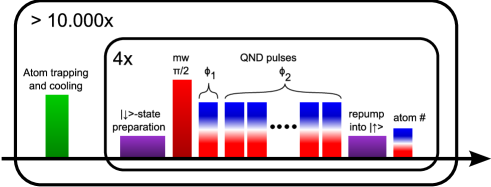
Figure 1: Experimental pulse sequence for the preparation of a coherent spin state and quantum non-demolition measurements.

To ensure that the microwave does not adress hyperfine transitions other than the clock transition, the bias magnetic field $B$ is set so that the Zeeman splitting $\Delta E_{Z}$ between adjacent magnetic sublevels ($350\,\mathrm{kHz/G}$ to first order) coincides with one of the zeroes of the microwave pulses’ frequency spectrum: $\Delta E_{Z}=\ell/\tau_{\pi/2}$, where $\tau_{\pi/2}$ is the microwave $\pi/2$ pulse duration, and $\ell$ is an integer number. Therefore for typical durations of $\tau_{\pi/2}=7\,\mathrm{\mu s}$, we set the bias magnetic field to $1.22\,\mathrm{G}$.

2.3 Dispersive population measurement

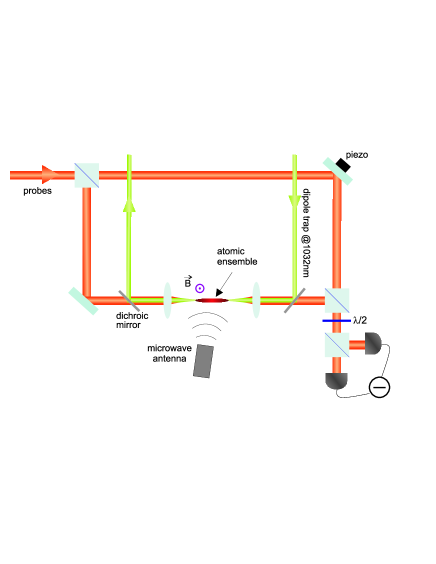
Figure 2: Mach-Zehnder interferometer. The atoms are placed in one arm of a Mach-Zehnder interferometer. The dipole trapping beam is overlapped with the probe arm to form an elongated atomic cloud along the propagation direction of the probe beam. Two probe beams of identical linear polarization enter the interferometer via the same input port and acquire phase shifts proportional to the number of atoms in the clock states $N_{\uparrow}$ and $N_{\downarrow}$, respectively. The bias magnetic field (B) is aligned to the polarization of the probe beams.

In order to measure an atomic squeezed state, we require a measurement sensitivity that is sufficient to reveal the atomic projection noise limit. The population in each clock level is measured via the phase shift imprinted on a dual-color beam propagating through the atomic cloud [28]. The dipole trap is overlapped with one arm of a Mach-Zehnder interferometer (see Fig. 2). A beam $P_{\downarrow}$ of one color off-resonantly probes the $\left|F=3\right>\rightarrow\left|F^{\prime}=2\right>$ transition, whereas a second beam $P_{\uparrow}$ off-resonantly probes the $\left|F=4\right>\rightarrow\left|F^{\prime}=5\right>$ transition (see Fig. 3). Each color experiences a phase shift proportional to the number of atoms in the ground state of the probed transition: $\phi_{\downarrow}=\chi_{\downarrow}N_{\downarrow}$ and $\phi_{\uparrow}=\chi_{\uparrow}N_{\uparrow}$ [29]. We carefully choose the probe detunings to ensure that the coupling constants are equal: $\chi_{\uparrow}=\chi_{\downarrow}$. The two probe beams emerge from one single-mode polarization maintaining fiber, and their intensities are stabilized to be equal $n_{\uparrow}=n_{\downarrow}$ to within $0.1\%$.

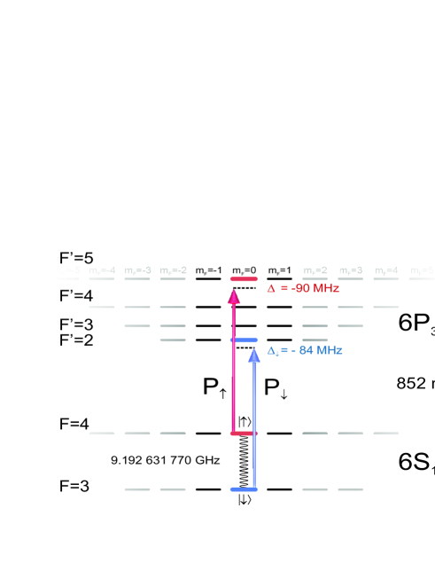
Figure 3: Cesium $D_{2}$-line level diagram

For each individual probe, the photocurrent difference between the detectors at the two output ports of the interferometer reads as:

$$\Delta n_{\uparrow}=n_{\uparrow}\beta\cos(k_{\uparrow}\Delta L+\chi_{\uparrow}N_{\uparrow})\textrm{ and }\Delta n_{\downarrow}=n_{\downarrow}\beta\cos(k_{\downarrow}\Delta L+\chi_{\downarrow}N_{\downarrow}),$$ (2)

where $k_{\uparrow},k_{\downarrow}$ are the wave vector lengths for $P_{\uparrow},P_{\downarrow}$, respectively, $\Delta L$ is the interferometer path length difference and $\beta=\sqrt{13}$ is the ratio of the field amplitudes in the reference- and probe-arm of the interferometer. In the absence of atoms $N_{\uparrow}=N_{\downarrow}=0$; therefore the smallest interferometer path length difference which leads to opposite phase for the signals $\Delta n_{\uparrow}$ and $\Delta n_{\downarrow}$ is: $\Delta L_{0}=\frac{\pi}{k_{\uparrow}-k_{\downarrow}}$. Since the wavelengths of the two probe lasers are so close (to one part in $40\,000$), one can assume that the fringes of each color are of opposite phase in the neighborhood of several wavelengths around $\Delta L_{0}$. The interferometer path length difference clock4.bib[\niib@name1] is set to the value closest to $\Delta L_{0}$ that also satisfies: $\Delta n_{\uparrow}=\Delta n_{\downarrow}=0$. This path length difference therefore varies with the expected atom number. To account for technical imperfections in the balancing of the probe powers and frequencies we define the average effective coupling strength $n\chi\equiv(n_{\uparrow}\chi_{\uparrow}+n_{\downarrow}\chi_{\downarrow})/2$ and the balancing error $n\Delta\chi\equiv(n_{\uparrow}\chi_{\uparrow}-n_{\downarrow}\chi_{\downarrow})/2$ as well as the average intensity $n=(n_{\uparrow}+n_{\downarrow})/2$.

This way, the total photocurrent difference $\Delta n=\Delta n_{\uparrow}+\Delta n_{\downarrow}$ reads as:

$$\Delta n=n_{\uparrow}\beta\sin(\chi_{\uparrow}N_{\uparrow})-n_{\downarrow}\beta\sin(\chi_{\downarrow}N_{\downarrow})\simeq n\beta(\chi\,\Delta N+\Delta\chi\,N_{A}).$$ (3)

We define the phase measurement outcome as:

$$\phi\equiv\frac{\Delta n}{\beta n}=\frac{\delta n}{\beta n}+\chi\,\Delta N+\Delta\chi\,N_{A},$$ (4)

where $\delta n$ denotes the total shot noise contribution from both colors. The phase $\phi$ provides a measurement of $\Delta N$ with added shot noise and classical noise. For $N_{A}$ atoms in a CSS, we have $\mathrm{var}(\Delta N)=N_{A}$. The projection noise increases with the atom number and using $\langle\Delta\chi\rangle=0,\langle\Delta N\rangle=0$ we obtain:

$$\mathrm{var}(\phi)=\frac{\beta^{2}+1}{2\beta^{2}}\,\frac{1}{n}+\chi^{2}N_{A}+\mathrm{var}(\Delta\chi)\,{N_{A}}^{2}.$$ (5)

After each experiment we use the same dual-color probe beam to determine the total atom number $N_{A}$. To that end we first optically pump all atoms into $\left|F=4,m_{F}=-1,0,+1\right>$. The phase measurement outcome reads as $\phi=n\bar{\chi}N_{A}$, where $\bar{\chi}$ is the effective coupling constant for the probe $P_{\uparrow}$, when the atoms are distributed among different magnetic sublevels. The similarity of the Clebsch-Gordan coefficients for the $\left|F=4,m_{F}\right>\rightarrow\left|F^{\prime}=5,m_{F}\right>$ transitions (with low $|m_{F}|$) ensures that $\bar{\chi}\approx\chi$ which is confirmed by experiments with a precision of better than $5\,\mathrm{\%}$.

2.4 Projection noise measurements

The two probe beams are generated by two extended-cavity diode lasers, which are phase-locked in order to minimize their relative frequency noise [31]. Their detunings are given in Fig. 3.

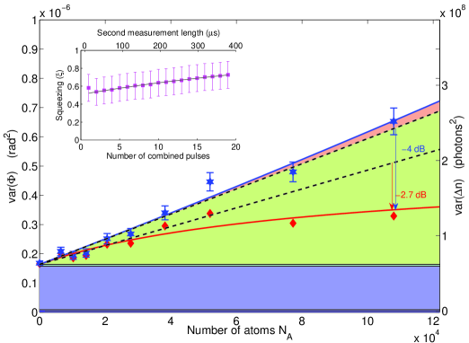
Figure 4: Projection noise and spin squeezing. The first QND measurement is performed with a $10~{}\mu$s bichromatic pulse containing $6\cdot 10^{6}$ photons in total. The second measurement is comprised of two such pulses. Blue stars: variance of the second measurement $\mathrm{var}(\phi_{2})$, where the data are sorted by atom number and grouped into 10 bins. Solid blue line: quadratic fit to $\mathrm{var}(\phi_{2})$. Green area: atomic projection noise of the CSS. Red diamonds: conditional variance $\mathrm{var}(\phi_{2}-\zeta\phi_{1})$. Red line: reduced noise as predicted by the fits to the noise data. The error bars correspond to the statistical uncertainty given by the number of measurements. This data is obtained by acquiring 1200 MOT loading cycles, i.e. 4800 experiments. Inset: metrologically relevant spin squeezing $\xi$ (as defined in Eq. 1) as a function of the number of pulses combined to form the second measurement. The data is fitted with an exponential decay (solid line).

In Fig. 4, we analyze the variance of the atomic population difference measurement as a function of the atom number.

As the data acquisition proceeds over several hours, it is a major challenge to keep experimental parameters such as $\tau_{\pi/2}$ constant to much better than $1/\sqrt{N_{A}}$ so that the mean values of the atomic population difference measurements would not drift by more than their quantum projection noise. To eliminate the influence of such slow drifts, we subtract the outcomes of measurements performed on independent atomic ensembles recorded in successive MOT cycles from each other. We then calculate the variances using this differential data.

The correlated and uncorrelated parts of the noise variance are fitted with second order polynomials. According to Eq. 5, we interpret the linear part of this fit as the CSS projection noise contribution. We observe a negligible quadratic part which means that classical noise sources like laser intensity and frequency fluctuations, which cause noise in the effective coupling constant are small. Achieving this linear noise scaling is a significant experimental challenge (see [12, Suppl.]), since the effect on $\Delta N$ of various sources of classical noise must be kept well below the level of $1/\sqrt{N_{A}}\simeq 3\cdot 10^{-3}$ between independent measurements, i.e. over a duration of $\simeq 5\,\mathrm{s}$.

2.5 Conditional noise reduction

Both measurements $\phi_{1}$ and $\phi_{2}$ are randomly normally distributed around zero with variances that have contributions from the shot noise and the atomic projection noise:

$$\mathrm{var}(\phi_{1})=\frac{1}{n_{1}}+\chi^{2}N_{A},\ \mathrm{var}(\phi_{2})=\frac{1}{n_{2}}+\chi^{2}N_{A}.$$ (6)

Since the two measurements are performed on the same atomic sample, they are correlated: $\mathrm{cov}(\phi_{1},\phi_{2})=\chi^{2}N_{A}$. The conditional variance $\mathrm{var}(\phi_{2}-\zeta\phi_{1})$ is minimal when $\zeta=\frac{\mathrm{cov}(\phi_{1},\phi_{2})}{\mathrm{var}(\phi_{1})}$:

$$\mathrm{var}(\phi_{2}-\zeta\phi_{1})=\frac{1}{n_{2}}+\frac{1}{1+\kappa^{2}}\chi^{2}N_{A}.$$ (7)

We measure $\kappa^{2}=1.6$ for $N_{A}=1.2\cdot 10^{5}$ atoms and we obtain a reduction of the projection noise by $\frac{1}{1+\kappa^{2}}=-4$ dB compared to the CSS projection noise, as indicated by the blue arrow in Fig. 4.

2.6 Decoherence

Dispersive coupling is inevitably accompanied by spontaneous photon scattering, inducing atomic population redistribution among the ground magnetic sublevels, as well as a reduction of coherence between the clock levels. Due to the selection rules, the population redistribution predominantly occurs within the Zeeman structure of the hyperfine levels [28]: Atoms that scatter a photon from the $P_{\downarrow}$ probe almost certainly end up in the $\left|F=3,m_{F}=-1,0,+1\right>$ sublevels again and atoms that scatter a photon from the $P_{\uparrow}$ probe predominantly end up in the $\left|F=4,m_{F}=-1,0,+1\right>$ states (see. Fig. 3). More importantly, the similarity of the Clebsch-Gordan coefficients that describe coupling of the probe light to low $|m_{F}|$-sublevel states ensures that the optical phase shift is almost unaffected by such a population redistribution. This makes our dual-color measurement an almost ideal QND-measurement as spontaneous scattering events effectively do not change the outcome of a $J_{z}$ measurement, i.e. no extra projection noise due to repartition into the opposite hyperfine ground states is added. On the other hand, the spontaneous photon scattering still leads to a shortening of the mean collective spin vector $\langle J\rangle\rightarrow(1-\eta)\langle J\rangle$.

The photon-number dependence of this mechanism can be modeled as $\eta=1-e^{\alpha n}$, where $n$ is the total number of photons in the probe pulse. We measure the parameter $\alpha$ in a separate experiment, by comparing the Ramsey fringe amplitudes with and without a bichromatic QND pulse between the two microwave $\pi/2$-pulses, as shown in Fig. 5. We obtain a value of $\alpha=-2.39\cdot 10^{-8}$ for this particular atomic cloud geometry.

(a)

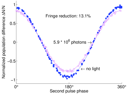
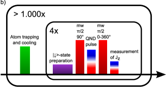
Figure 5: Decoherence measurement via Ramsey fringe reduction. (a) Blue points: full Ramsey fringe. Red points: reduced fringe when a QND-pulse containing $5.9\cdot 10^{6}$ photons is inserted in the Ramsey sequence. In this experiment, the fringe height is reduced by $13.1\%$, leading to a decoherence parameter $\alpha=2.39\times 10^{-8}$. (b) Pulse sequence.

Each probe color induces an inhomogeneous ac Stark shift on the atomic levels, causing additional dephasing and decoherence. Nevertheless, in our two-color probing scheme, the Stark shift on level $\left|\uparrow\right>$ caused by probe $P_{\uparrow}$ is compensated by an identical Stark shift on level $\left|\downarrow\right>$ caused by probe $P_{\downarrow}$, provided the probe frequencies are set so that $\chi_{\uparrow}=\chi_{\downarrow}$, and the probe powers are equal. Hence, the two Ramsey fringes depicted on Fig. 5 (with and without a light pulse) are in phase to better than $1^{\circ}$.

2.7 Squeezing and entanglement

A QND measurement is characterized by the decoherence $\eta$ it induces, and by the $\kappa^{2}$-coefficient that describes the measurement strength. In the absence of classical noise, for the dual-color QND the squeezing parameter as defined in Eq. 1 can be written as:

$$\xi_{\textrm{\footnotesize lin}}=\frac{1}{(1-\eta)^{2}\,(1+\kappa^{2})}.$$ (8)

Therefore, for a fixed detuning of the laser frequencies, the choice of the number of photons used in a QND measurement is the result of a trade-off between the amount of decoherence induced by the photons and the amount of information that the $\phi_{1}$-measurement yields [32].

Here, we use $n_{1}/2=3\cdot 10^{6}$ photons per probe color, inducing a shortening of $\eta=14\%$ of the collective spin $J$. From Eq. 8 we expect an improvement of the signal-to-projection-noise ratio by $1/\xi_{\textrm{\footnotesize lin}}=2.8$ dB compared to a CSS. From the data presented in Fig. 4 we measure $1/\xi=2.7$ dB, as indicated with a red arrow. This value agrees well with the theory and with the results reported in [12].

The detuning of the probe light with respect to the atomic transitions (see Fig. 3) as well as the duration of the probe pulses ($10\,\mathrm{\mu s}$) have been chosen to minimize the influence of classical noise sources such as electronic noise in the detector and relative frequency- and intensity-noise of the two probe colors.

Since the probe pulses redistribute population only within the hyperfine manifold (cf. sec. 2.6), the light shot noise contribution in the second measurement variance can be reduced by increasing the number of photons $n_{2}$ in the second measurement (cf. Eq. 8). In our experiment, the second measurement is comprised of $10\,\mathrm{\mu s}$ long bichromatic pulses containing a total of $n_{2}$ photons, separated by $10~{}\mu$s. As shown in the inset of Fig. 4, $\xi$ exponentially approaches unity as more pulses are combined to form the second measurement. We attribute this decay to the atomic motion within the dipole trap during the second measurement: the atoms move in the transverse profile of the probe beam, and are probed with a position dependent weight corresponding to the local probe light intensity. Movement during the time interval between the first and second probe pulse therefore induces a decay of the correlations between the two measurements. We fit the experimental data with:

$$\xi(t_{2})=1-Be^{-t_{2}/\tau_{\mathrm{decay}}},$$ (9)

where $t_{2}$ is the total duration of the second measurement, and obtain $\tau_{\mathrm{decay}}=670\,\mathrm{\mu s}$, which is of the same order of magnitude as half the radial trap oscillation period [33].

3 Entanglement-assisted atomic clock

3.1 Entanglement-assisted Ramsey sequence

We use the spin squeezing technique described in the previous section to improve the precision of a Ramsey clock. The modified Ramsey sequence is shown in Fig. 6. As in a traditional Ramsey sequence, all atoms are prepared in $\left|\downarrow\right>$ initially. A near-resonant $\pi/2$-pulse with a phase of $\vartheta_{0}=90^{\circ}$ and detuning $\Delta$ drives them into a CSS with macroscopic $J_{x}=\frac{N_{A}}{2}$ (Fig. 6.a). This state is then squeezed along the $z$-direction by performing a weak QND measurement of the pseudo-spin component $J_{z}$ (Fig. 6.b). This population-squeezed state is converted into a phase-squeezed state by a second $\pi/2$-pulse with phase $\vartheta_{1}=0^{\circ}$ that rotates the state around the $x$-axis. At this point, the Ramsey interrogation time starts (Fig 6.c.1). We let the atoms evolve freely for a time $T$, during which they acquire a phase proportional to the microwave detuning $\varphi=\Delta\,T$ (Fig 6.c.2). To stop the clock, a third $\pi/2$-pulse with phase $180^{\circ}$ is applied, converting the accumulated atomic phase shift $\varphi$ into a population difference (Fig 6.c.3). Finally, we measure the $J_{z}$-spin component a second time and from the two measurement outcomes we compute the conditional variance $\mathrm{var}{(\phi_{2}-\zeta\phi_{1})}$.

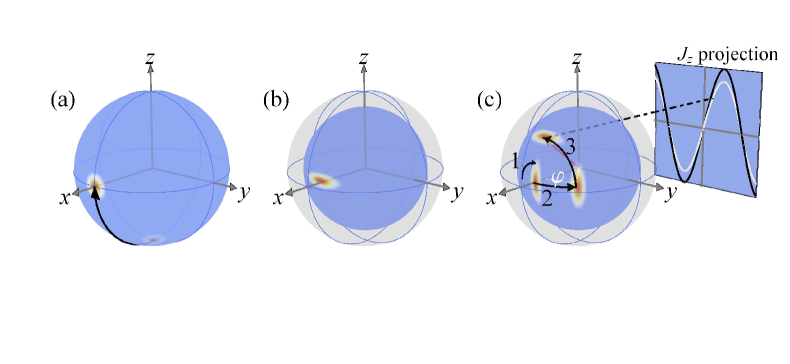
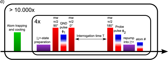
Figure 6: Ramsey sequence including squeezing in the Bloch sphere representation. The sequence starts with all atoms in $\left|\downarrow\right>$. (a) A near resonant $\pi/2$-pulse is applied with phase $\vartheta_{0}=90^{\circ}$, placing the atoms in a coherent spin state along the $x$-axis. (b) The atomic state is squeezed along the $z$-direction by a weak QND measurement of the population difference. The decoherence induced by the first QND measurement leads to a reduction of the Bloch sphere radius. (c.1) A second $\pi/2$-pulse with phase $\vartheta_{1}=0^{\circ}$ rotates the atomic state around the $x$-axis, thus converting the population squeezing into phase squeezing. (c.2) Free precession during interrogation time $T$, equivalent to a rotation around the $z$-axis by an angle $\varphi=\Delta\,T$. (c.3) A third $\pi/2$-pulse, with phase $\vartheta_{2}=180^{\circ}$, acts as a $\pi/2$-rotation around the $x$-axis. The final state has a $z$-axis component $\langle J_{z}\rangle=(1-\eta)\frac{N_{A}}{2}\sin\varphi$. The reduction of the atomic projection noise results in a reduced uncertainty in the measurement of $\phi_{2}$. (d) Diagram of the pulse sequence.

The first QND measurement of $J_{z}$ shown in Fig.6.b induces decoherence that reduces the pseudo-spin vector length, and hence the Ramsey fringe height, so that:

$$\langle J_{z}\rangle=(1-\eta)\frac{N_{A}}{2}\sin\varphi,$$ (10)

in contrast to the Ramsey fringe height in the absence of a QND measurement: $\langle J_{z}\rangle=\frac{N_{A}}{2}\sin\varphi$. Therefore, a QND measurement reduces the clock phase-sensitivity (given by the Ramsey signal slope $d\phi/d\varphi)$ by a factor $1-\eta$. Tailoring the QND measurement strength induces squeezing, and thus improves the signal-to-projection-noise ratio by $1/\xi$ in variance as given in Eq. 1.

We emphasize that atoms that have undergone spontaneous emissions into the $m_{F}\neq 0$ states do not take part in the clock rotations: Due to the magnetic bias field the microwave radiation only couples the $\left|F=3,m_{F}=0\right>$ to the $\left|F=4,m_{F}=0\right>$ state. These atoms are however part of the entangled state as they carry some part of the information of the QND measurement outcome: Only when these atoms are measured together with the $m_{F}=0$-atoms in the second measurement there is no additional partition noise due to spontaneous emissions. It is therefore important that in the absence of a phase shift ($\varphi=0$) the rotation operator corresponding to our microwave clock pulse sequence commute with $J_{z}$, i.e. the population difference $\Delta N$ is not changed.

3.2 Low phase noise microwave source

A projection noise limited atomic clock with $N_{A}=10^{5}$ atoms can resolve atomic phase fluctuations as small as $\delta\varphi=1/\sqrt{N_{A}}=3\,\mathrm{mrad}$. This poses strict requirements on the phase noise of our microwave oscillator: during the interrogation time its phase has to be much more stable than $1/\sqrt{N_{A}}$ so that our clock performance is not limited by the oscillator. For an oscillator with a white phase noise spectrum and for a clock interrogation time of $T=10\,\mathrm{\mu s}$ this translates into a required relative phase noise power density lower than $-100\,\mathrm{dBc/Hz}$ over a 100 kHz sideband next to the 9.192 GHz carrier. This is more than one order of magnitude smaller than the phase noise of the Agilent HP8341B microwave synthesizer used in [12].

A key step in the implementation of the clock sequence therefore was the construction of a low-noise synthesizer chain: a 9 GHz dielectric resonator oscillator (DRO-9.000-FR, Poseidon Scientific Instruments) with a phase noise of $-132\,\mathrm{dBc/Hz}@100\,\mathrm{kHz}$ is phase locked to an oven-controlled 500 MHz quartz oscillator (OCXO) (MV87, Morion Inc.) within a bandwidth of 15 kHz. The OCXO itself is slowly $(\approx 10\,\mathrm{Hz})$ locked to a GPS reference. A direct digital synthesis (DDS) board (Analog Devices AD9910) is clocked from the frequency doubled OCXO and produces a 192 MHz signal which is mixed onto the DRO output; a microwave cavity resonator, with a 50 MHz width, filters out the upper 9.192 GHz sideband. By using the DDS to shape the microwave pulses we control the microwave pulse duration with a precise timing in 4 ns steps and control the microwave phase digitally with a ${2\pi\cdot 2^{-16}\,\mathrm{rad}}$ resolution, allowing for complex and precise pulse sequences.

3.3 Ramsey fringe decay

We first operate our clock with the sequence described in Fig. 6, leaving out the first QND measurement. The phase $\vartheta_{2}$ of the last microwave pulse is varied between $0^{\circ}$ and $360^{\circ}$. The microwave frequency is set to resonance (to within $10$ Hz), so we expect $\langle J_{z}\rangle=\frac{N_{A}}{2}\cos\vartheta_{2}$. In Fig. 7, we plot the distribution of $J_{z}$-measurements normalized to $\langle J\rangle=N_{A}/2$, for different interrogation times $T$ between $10\,\mathrm{\mu s}$ and $350\,\mathrm{\mu s}$. The differential ac Stark shift induced by the Gaussian dipole trap potential causes spatially inhomogeneous dephasing during the whole interrogation time $T$. This results in a decay of the Ramsey fringe contrast $h(T)$ (and therefore a decay of the clock phase sensitivity) as $T$ increases, as shown in Fig. 7.

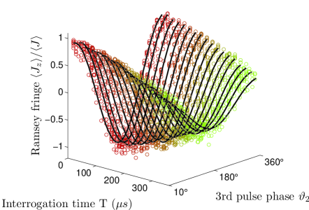
(a) (b)

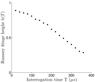
Figure 7: (a) Ramsey fringe for interrogation times ranging from $10\,\mathrm{\mu s}$ (red points) to $350\,\mathrm{\mu s}$ (green points). Solid lines: fits of type $\langle J_{z}\rangle/\langle J\rangle=h(T)\cos\vartheta_{2}$ to the data. (b) Fringe contrast $h(T)$ derived from the fits in (a).

3.4 Ramsey sequence with squeezing

We implement the full EAR sequence described in Fig. 6, and keep the last microwave pulse phase $\vartheta_{2}=180^{\circ}$. The noise contributions to the second QND measurement are shown in Fig. 8. With such a short interrogation time ($10~{}\mu$s), only little classical noise is added to the second measurement, compared to the first measurement ($\mathrm{var}(\phi_{1})\approx\mathrm{var}(\phi_{2})$). We attribute this classical noise to microwave frequency noise and dipole trap intensity fluctuations.

Using the first weak measurement $\phi_{1}$ to predict the outcome of the second measurement $\phi_{2}$, we observe a metrologically relevant noise reduction of $\xi=-1.1\,\mathrm{dB}$ for $9\cdot 10^{4}$ atoms. This gives us the signal-to-projection-noise ratio improvement that we gained by running our clock with an entangled atomic ensemble, compared to a standard clock operating with unentangled atoms (see Fig. 8). The experimentally observed squeezing is lower than the expected value $\xi_{\textrm{\footnotesize lin}}=[(1-\eta)^{2}(1+\kappa^{2})]^{-1}=-2.2~{}$dB because of the extra classical noise in the second measurement $\phi_{2}$.

Note that the obtained squeezing is different from the one shown in Fig. 4. Apart from the fact that the atom number used in the clock experiment is lower, the reduction of the spin squeezing can be explained by two experimental effects: firstly, the atomic motion in the trap results in a decay of the correlations $\mathrm{cov}(\phi_{1},\phi_{2})$ during the the longer time interval between the two QND measurements $\phi_{1},\phi_{2}$ in the clock sequence. Secondly, in the Ramsey sequence, phase- and frequency fluctuations between atoms and the microwave oscillator affect the $\phi_{2}$ measurement to first order (cf. Eq. 10), whereas they only appear in second order in the simple squeezing sequence shown in Fig.1.

The first QND measurement $\phi_{1}$ also produces backaction antisqueezing on the conjugate spin variable $J_{x}$. Classical fluctuations in relative intensities of the two probe colors lead to a fluctuating differential AC-Stark shift between the clock levels. This adds additional noise to $J_{x}$, so that the produced SSS is about 10 dB more noisy in the (anti-squeezed) $J_{x}$ quadrature than a minimum uncertainty state. However, this excess noise does not affect the clock precision since we only perform $J_{z}$ measurements.

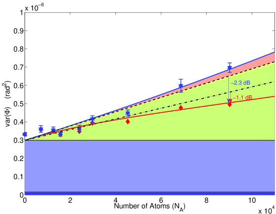
Figure 8: Noise contributions to the second measurement in the clock sequence, with an integration time of $T=10~{}\mu$s. The first measurement contains $7.1\cdot 10^{6}$ photons and induces a Bloch vector shortening of $13.5\%$.

3.5 Frequency noise measurements

The Ramsey sequence makes it possible to use an atomic ensemble either as a clock, where the frequency of an oscillator is locked to the transition frequency between the clock states $\nu=(E_{\uparrow}-E_{\downarrow})/h$, or as a sensor to measure perturbations of the energy difference between these levels. In our experiment, the atomic ensemble is sensitive to fluctuations of the frequency difference $\Delta$ between the cesium clock transition and the microwave oscillator.

The atomic transition frequency of $9\,192\,630\,500\,\mathrm{Hz}$ as measured in our experiments has a systematic offset from the SI value of $9\,192\,631\,770\,\mathrm{Hz}$ mainly for two reasons: firstly, the bias field of $\approx 1\,\mathrm{G}$ causes a quadratic Zeeman shift of $+427\,\mathrm{Hz/G^{2}}$ on the clock levels. Secondly, the trapping light produces a differential ac Stark shift of the order of $-1700\,\mathrm{Hz}$ averaged over the atoms within the probe beam. Noise in the phase evolution between the atoms and the microwave oscillator leads to added classical noise in the $\phi_{2}$ measurement, which scales as ${N_{A}}^{2}$.

The frequency noise components that an atomic clock can detect are determined by the clock’s cycle time $t_{c}$, and the interrogation time $T$. Uncorrelated frequency fluctuations from cycle to cycle result in additional noise in the $\phi_{2}$-measurement that scales as $T^{2}$ in variance. Phase noise between atoms and the microwave oscillator during the interrogation time $T$, however, can follow a different scaling behaviour. Since we subtract the outcomes of successive MOT loading-cycles, our clock is not sensitive to any frequency noise slower than $t_{c}=5\,\mathrm{s}$.

3.6 Influence of classical noise on the clock performance

The quantum noise limited frequency sensitivity of an atomic clock improves with increasing the interrogation time. However, achieving a higher frequency sensitivity makes our experiment more susceptible to classical noise. In order to evaluate the limitations of our proof-of-principle experiment, we vary the interrogation time $T$ from $10\,\mathrm{\mu s}$ to $310\,\mathrm{\mu s}$ by steps of $20~{}\mu$s, while keeping the atom number approximately constant at $N_{A}=9\cdot 10^{4}$. From the optical phase shift measurements $\phi_{1}$ and $\phi_{2}$, we can infer the atomic phase evolution by normalizing to the Ramsey fringe amplitude and define:

$$\tilde{\varphi}_{2}=\frac{\phi_{2}}{A(T)}\qquad\tilde{\varphi}_{21}=\frac{\phi_{2}-\zeta\phi_{1}}{A(T)}.$$ (11)

where $A(T)=\chi\,(1-\eta)\,h(T)\,N_{A}$ and $h(T)$ is the Ramsey fringe contrast shown in Fig. 7.

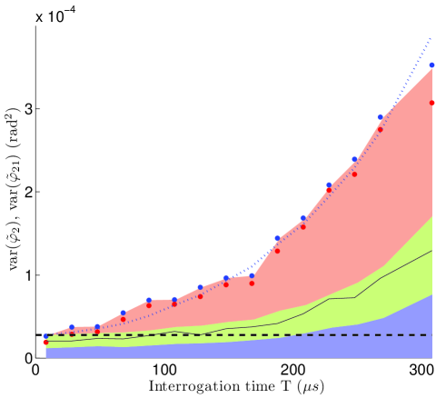
Figure 9: Contributions to the atomic phase noise as a function of the interrogation time $T$. Blue points: $\mathrm{var}(\tilde{\varphi}_{2})$. Red points: $\mathrm{var}(\tilde{\varphi}_{21})$. For each interrogation time $T$, we determine the various noise contributions to $\mathrm{var}(\phi_{2})$, as shown in Fig. 8. Using Eq. 11, we obtain the noise contributions to $\mathrm{var}(\tilde{\varphi}_{2})$. The different contributions to $\mathrm{var}(\tilde{\varphi}_{2})$ are: the shot noise (blue area), projection noise (green area), and classical noise (red area). The dotted line is a quadratic fit to the classical noise contribution to $\mathrm{var}(\tilde{\varphi}_{21})$ (red area). The solid line shows the reduced projection noise which would be obtainable in the absence of classical noise. The dashed line demarcates the area in which the Wineland criterion (cf. Eq. 1) is satisfied $\mathrm{var}(\tilde{\varphi}_{21})<1/N_{A}$, corresponding to the regime of metrologically relevant squeezing. In the absence of classical noise, the maximum interrogation time at which the Wineland criterion would be satisfied is given by the intersection between the dashed and solid lines at $T=90\,\mathrm{\mu s}$.

In Figure 9, we plot the measured atomic phase noise variance $\mathrm{var}(\tilde{\varphi}_{2})$ and the conditionally reduced noise of the atomic phase $\mathrm{var}(\tilde{\varphi}_{21})$ as a function of the interrogation time $T$. Only in the first data point (corresponding to $T=10\,\mathrm{\mu s}$) we observe squeezing, i.e. the measured noise in $\tilde{\varphi}_{21}$ is lower than that of a traditionally operated atomic clock with an identical signal-to-projection-noise ratio (i.e. with an atom number of $N_{A}/\xi_{\textrm{\footnotesize lin}}$).

We observe a quadratic increase in the classical noise with $T$. This suggests that the detuning is roughly constant over the interrogation time, but varies from cycle to cycle. We attribute these fluctuations to both intensity drifts in the dipole trap and variations of the geometry of the atomic cloud. From the fit (solid green line) we infer $\sqrt{\mathrm{var}(\Delta)}=7.5\,\mathrm{Hz}$ per cycle.

4 Conclusion

In summary, we have demonstrated the first entanglement-assisted Ramsey clock, following the proposal of [12]. We have implemented a modified Ramsey sequence in which the spin state is squeezed by means of a quantum non-demolition measurement. Squeezing results in a metrologically relevant reduction of the noise variance by $-1.1\,\mathrm{dB}$ with $9\cdot 10^{4}$ atoms, compared to a traditional atomic clock at the projection noise limit with the same number of atoms. The present experimental developments have been made possible by the introduction of a low phase noise microwave source.

The dual-color QND method implemented in this work is readily applicable to optical clocks as well. The idea of using quantum non-demolition measurements to generate entanglement and to improve the precision of a clock has drawn the attention of the ultra-precise-frequency-standards community [8, 13]. Besides, non-destructive measurements have been shown to drastically improve the duty cycle in a clock experiment, thereby reducing the Dick effect [13].

We have shown that for the present proof-of-principle experiment, the improvement of the clock precision due to squeezing does not extend to interrogation times beyond $10\,\mathrm{\mu s}$. This is due to the inhomogeneous broadening on the hyperfine transition induced by the dipole trap, and the fact that large interrogation times make the clock more sensitive to light shifts induced by cloud-geometry- and intensity fluctuations in the dipole trap. These issues could be circumvented by turning to systems for which there exists a magic wavelength, such as strontium [34, 35] or ytterbium[36]. For long interrogation times, the clock performance also is limited by the atomic motion, which can be counteracted by introducing a transverse optical lattice.

The figure of merit for the QND-induced spin squeezing is the resonant optical depth of the atomic ensemble. In the present experiment the optical depth was limited to a value $\approx 10$. Implementation of QND-based spin squeezing in state-of-the-art clocks will require solutions where high optical depth can be combined with low collisional broadening, such as, for example, optical lattices placed in a low finesse optical cavity.

References

References

- [1] G. Santarelli, P. Laurent, P. Lemonde, A. Clairon, A. G. Mann, S. Chang, A. N. Luiten, and C. Salomon, Phys. Rev. Lett. 82, 4619 (1999).
- [2] G. Wilpers, T. Binnewies, C. Degenhardt, U. Sterr, J. Helmcke, and F. Riehle, Phys. Rev. Lett. 89, 230801 (2002).
- [3] A. D. Ludlow, T. Zelevinsky, G. K. Campbell, S. Blatt, M. M. Boyd, M. H. G. de Miranda, M. J. Martin, J. W. Thomsen, S. M. Foreman, J. Ye, T. M. Fortier, J. E. Stalnaker, S. A. Diddams, Y. L. Coq, Z. W. Barber, N. Poli, N. D. Lemke, K. M. Beck, and C. W. Oates, Science 319, 1805 (2008).
- [4] D. J. Wineland, J. J. Bollinger, W. M. Itano, F. L. Moore, and D. J. Heinzen, Phys. Rev. A 46, R6797 (1992).
- [5] S. F. Huelga, C. Macchiavello, T. Pellizzari, A. K. Ekert, M. B. Plenio, and J. I. Cirac, Phys. Rev. Lett. 79, 3865 (1997).
- [6] V. Giovannetti, S. Lloyd, and L. Maccone, Science 306, 1330 (2004).
- [7] A. André, A. S. Sørensen, and M. D. Lukin, Phys. Rev. Lett. 92, 230801 (2004).
- [8] D. Meiser, J. Ye, and M. J. Holland, New J. Phys. 10, 073014 (2008).
- [9] V. Meyer, M. A. Rowe, D. Kielpinski, C. A. Sackett, W. M. Itano, C. Monroe, and D. J. Wineland, Phys. Rev. Lett. 86, 5870 (Jun 2001).
- [10] W. Wasilewski, K. Jensen, H. Krauter, J. Renema, M. V. Balabas, and E. Polzik, “Quantum noise limited and entanglement-assisted magnetometry,” arXiv:0907.2453v3.
- [11] M. Koschorreck, M. Napolitano, B. Dubost, and M. W. Mitchell, “Measurement of spin projection noise in broadband atomic magnetometry,” arXiv:0911.4491v1.
- [12] J. Appel, P. J. Windpassinger, D. Oblak, U. B. Hoff, and N. Kjærgaard, Proc. Natl. Acad. Sci. 106, 10960 (2009).
- [13] J. Lodewyck, P. G. Westergaard, and P. Lemonde, Phys. Rev. A 79, 061401 (2009).
- [14] W. M. Itano, J. C. Bergquist, J. J. Bollinger, J. M. Gilligan, D. J. Heinzen, F. L. Moore, M. G. Raizen, and D. J. Wineland, Phys. Rev. A 47, 3554 (1993).
- [15] A. Sørensen, L.-M. Duan, J. I. Cirac, and P. Zoller, Nature 409, 63 (2001).
- [16] J. Estève, C. Gross, A. Weller, S. Giovanazzi, and M. K. Oberthaler, Nature 455, 1216 (2008).
- [17] A. Kuzmich, K. Mølmer, and E. S. Polzik, Phys. Rev. Lett. 79, 4782 (1997).
- [18] J. Hald, J. L. Sørensen, C. Schori, and E. S. Polzik, Phys. Rev. Lett. 83, 1319 (1999).
- [19] J. Appel, E. Figueroa, D. Korystov, M. Lobino, and A. I. Lvovsky, Phys. Rev. Lett 100, 093602 (2008).
- [20] K. Honda, D. Akamatsu, M. Arikawa, Y. Yokoi, K. Akiba, S. Nagatsuka, T. Tanimura, A. Furusawa, and M. Kozuma, Phys. Rev. Lett. 100, 093601 (2008).
- [21] P. Grangier, J.-F. Roch, and G. Roger, Phys. Rev. Lett. 66, 1418 (1991).
- [22] A. Kuzmich, N. P. Bigelow, and L. Mandel, Europhys. Lett. 42, 481 (1998).
- [23] A. Kuzmich, L. Mandel, and N. P. Bigelow, Phys. Rev. Lett. 85, 1594 (2000).
- [24] S. Chaudhury, G. A. Smith, K. Schulz, and P. S. Jessen, Phys. Rev. Lett. 96, 043001 (2006).
- [25] M. H. Schleier-Smith, I. D. Leroux, and V. Vuletić, Phys. Rev. Lett. 104, 073604 (2010).
- [26] T. Takano, M. Fuyama, R. Namiki, and Y. Takahashi, Phys. Rev. Lett. 102, 033601 (2009).
- [27] B. Julsgaard, A. Kozhekin, and E. S. Polzik, Nature 413, 400 (2001).
- [28] M. Saffman, D. Oblak, J. Appel, and E. S. Polzik, Phys. Rev. A 79, 023831 (2009).
- [29] P. J. Windpassinger, D. Oblak, P. G. Petrov, M. Kubasik, M. Saffman, C. L. G. Alzar, J. Appel, J. H. Müller, N. Kjærgaard, and E. S. Polzik, Phys. Rev. Lett. 100, 103601 (2008).
- [30] In [12] we used opposite input ports for the two probe colors and operated the interferometer in its white-light position to minimize sensitivity to differential probe frequency noise. The method described here allows us to feed light of both probe colors into the interferometer through one common single mode fiber. This eliminates a possible spatial mode mismatch, which leads to spatially inhomogeneous differential AC-Stark shifts across the atomic sample. The differential probe frequency is controlled tightly using an optical phase lock [31].
- [31] J. Appel, A. MacRae, and A. I. Lvovsky, Meas. Sci. Technol. 20, 055302 (2009).
- [32] P. J. Windpassinger, D. Oblak, U. B. Hoff, A. Louchet, J. Appel, N. Kjærgaard, and E. S. Polzik, J. Mod. Opt. 56, 1993 (2009).
- [33] D. Oblak, J. Appel, P. Windpassinger, U. Hoff, N. Kjærgaard, and E. Polzik, Eur. Phys. J. D 50, 67 (2008).
- [34] H. Katori, M. Takamoto, V. G. Pal’chikov, and V. D. Ovsiannikov, Phys. Rev. Lett. 91, 173005 (2003).
- [35] J. Ye, H. J. Kimble, and H. Katori, Science 320, 1734 (2008).
- [36] Z. W. Barber, J. E. Stalnaker, N. D. Lemke, N. Poli, C. W. Oates, T. M. Fortier, S. A. Diddams, L. Hollberg, C. W. Hoyt, A. V. Taichenachev, and V. I. Yudin, Phys. Rev. Lett. 100, 103002 (Mar 2008).