On the possible critical behaviour of a marginally stable stellar disc

Abstract

Using hydrodynamic approach, it is shown that the properties of a marginally stable collisionless stellar disc resemble those of a thermodynamic system undergoing a gas–liquid phase transition. The maximum in Toomre’s stability diagram, which separates gravitationally stable and unstable states with respect to axisymmetric perturbations, can be treated as a critical point for this transition. Static perturbations of stellar density are explored and the mean perturbation amplitude is considered as the order parameter of the theory. The disc’s state is assumed to change as the disc passes through the critical point. Since the disc tends to retain hydrostatic equilibrium, structures can be formed spontaneously, identifiable with a seed spiral structure. A power-law scaling of the order parameter in the vicinity of the critical point has been found. The susceptibility and other Landau–Weiss exponents similar to those in the Van der Waals theory are calculated. The critical behaviour of marginally stable discs at the initial stage of their evolution occurs in numerical simulations where snapshots of stellar positions reveal stellar splinters and crescents diverging from the disc centre. These structures can be a result of the phase transition. In numerical simulations, these structures eventually reduce to decaying worm-type features because of the ‘heating’ most likely resulting from instability of stellar orbits due to resonances. Under favourable conditions the critical behaviour leading to the establishment of order in a stellar disc can result in the generation of a spiral structure.

Key words: galaxies: kinematics and dynamics – galaxies: spiral – galaxies: structure

1 Introduction

Our aim is to clarify whether an ordered state can arise spontaneously in a marginally stable stellar disc. We suggest that the marginal state can be a critical one with respect to a phase transition. We show that a self-gravitating galactic stellar disc is most sensitive to static perturbations of gravitational field at a certain length scale when the disc is in a marginal state (where chaotic stellar velocity is equal to the local gravitational momentum $\pi G\sigma/\kappa$, i.e., the mean gravity force times the epicycle period, where $G$ is Newton’s gravitational constant, $\sigma$ the surface mass density and $\kappa$ the epicyclic frequency). Perturbations of stellar density grow with the difference between the radial velocity dispersion and its Toomre’s characteristic value, and can modify the symmetry of the disc when their scale is comparable to the size of the stellar epicycle, the natural wavelength of oscillations.

The susceptibility of the stellar ‘gas’ is singular at the top point of the well-known Toomre’s stability diagram (Toomre 1964). Moreover, the static response to small perturbations of the gravitational potential can be singular in the region of instability in the diagram. Therefore internal physical equilibrium of a self-gravitating disc requires an analysis deeper than that in terms of the standard theory of dynamic instability.

Guided by physical considerations (Saslaw 1987), we assume that the marginal state of the disc is similar to a critical point of the gas–liquid phase transition (as a special case of the phase transition of the second kind), and the disc’s state in unstable region is similar to the condensed state of the van der Waals gas. (We stress that this is just a formal similarity; the physics of the stellar disc is quite different from that of a gas-liquid system.) Note, however, that we consider not the loss of thermodynamic stability as density increases, but rather the occurrence of a susceptible state, compressible and ‘elastic’ simultaneously. Therefore, the physical properties of perturbations in the ‘van der Waals region’ are analyzed using a nonlinear dependence of ‘pressure’ perturbations on stellar density perturbations. We demonstrate the possibility of a quasi-static compression of the perturbed stellar ‘gas’, obtain an equation for the order parameter (viz. the amplitude of the static perturbations in the stellar spatial density), and investigate the perturbations in the neighbourhood of the critical point in Toomre’s diagram.

In fact, a stellar disc is a collisionless dynamic system. The ‘elasticity’ of such a self-gravitating system results from both the epicyclic motions of stars under small perturbations and the centrifugal ‘elasticity’ of the reference (circular) stellar orbits themselves.

Although critical fluctuations can be important because of an anomalous behaviour of the susceptibility (Ivannikova, Ivanov & Maksumov 1994, 1997), we shall restrict ourselves to Landau’s approach and consider the possibility, for a self-gravitating stellar system, to reach a new local equilibrium by developing an ordered state. This approach uses an order parameter as a measure of evolution in the disc structure as it undergoes a phase transition, but fluctuations are ignored. Below we use the mean amplitude of density perturbations in the marginal disc as the order parameter. We do not use the method of thermodynamic potentials because of the well-known complications in its application to self-gravitating systems (Saslaw 1987).

As follows Saslaw’s arguments (§§29.1, 29.3, 30.3, and 31.1 in Saslaw 1987), a direct introduction of gravity into the theory of the van der Waals gas leads to a poor approximation, especially because of the collective nature of the gravitational interaction.

The method used here combines the mean field approach, similar to the mean molecular field theory of Weiss (§9.2 in Balescu 1975), and the ideas related to hydrostatic equilibrium in an external field and Landau’s theory of the gas–liquid phase transition. This differs from the fluctuational approach as the perturbations are considered to be ordered in space. It is assumed that all the stars are identical, and so each equally interacts with the other stars in the disc. This interaction is described by the mean field. This method is not free of disadvantages similar to those of the theories of van der Waals, Weiss and Landau.

In Section 2, density perturbation in the pre-critical state is obtained using linear collisionless hydrodynamics (theory of density waves, Lin & Shu 1964) and then its limiting value corresponding to the top point of Toomre’s diagram is taken. This approach is equivalent to the local gravithermodynamics, as shown by Saslaw (1987, §31) for the Jeans criterion as an example.

But the direct analysis of intrinsic (or proper internal) and forced static perturbations (as opposed to fluctuational ones) at the critical point in terms of general thermodynamic relations in Section 3 apparently provides the most straightforward explanation of the new phase in the marginally stable disc.

Our results, albeit schematic, clarify an important question as to how a self-gravitating disc will respond to a static spiral perturbation of gravitational potential (in the approximation of tight winding) whose wave number is equal to the inverse Coriolis radius and how the amplitude of stellar density perturbations will vary if the disc is close to the marginal stability (i.e., where the mean chaotic stellar velocity is comparable to the mean gravitational momentum acting on stars that move along the Coriolis circles). We assume that the response of the disc is similar to a phase transition of the second kind, and we use this assumption to suggest the form of the ‘pressure’ perturbations in the post-critical regime. The marginal state appears to be critical with respect to compression driven by the spiral perturbation of the gravitational potential, which can be expressed as a growth of the susceptibility of the stellar density perturbations. We recall that the critical point of the gas–liquid phase transition is characterized by the loss of thermodynamic stability as density increases.

The stellar disc in our theory does not have the van der Waals equation of state. We found it difficult to obtain any explicit form of the equation of state for the stellar disc. However, it is sufficient for our purposes to know the ‘pressure’ perturbation alone. Our main tools are Toomre’s stability diagram, the density wave theory, and the theory of critical phenomena due to van der Waals, Weiss and Landau. Important for the method used are Toomre’s critical dispersion (as an indicator of criticality), the mean field approach borrowed from the theory of stellar collective phenomena, and the ideas related to hydrostatic equilibrium in an external field.

We further assume that, in the critical region, the disc evolves into a new equilibrium state similarly to the van der Waals gas. Therefore we consider here static perturbations in the stellar disc. The amplitude of the perturbations is determined from equilibrium equations in a constant external and internal gravitational fields. We recall that Landau considered the thermodynamic potential for a fixed value of the order parameter determined from the minimum condition for the potential.

The concept of the critical point is modified because of the long-range nature of the gravitational force and the absence of stellar collisions (Saslaw 1987). An important role here is played by Toomre’s velocity dispersion, that is by the collective local interaction, rather than by pairwise interparticle interactions of van der Waals. The ‘centrifugal elasticity’ also results in a nonlinear term in the ‘pressure’ perturbation. We consider spontaneous condensations (‘convergence’) and rarification (‘divergence’) of stellar orbits in radius (similar to compressible perturbations in the van der Waals gas), but do not include such effects as ‘heating’.

2 The response function, coherence length and susceptibility in the pre-critical region

In this section we evaluate the response function using linear collisionless hydrodynamics including both forced and internal (proper) perturbations in the stellar spatial density.

Consider a nonaxisymmetric perturbation of the stellar surface density $\sigma_{m}$ (the order parameter), whose background value is $\sigma$, induced by small perturbations of gravitational potential $\psi_{1}=\psi_{1,\rm int}+\psi_{1,\rm ext}$ (positive definite), where the potential is represented as a sum of internal, self-consistent field and external field. In the limit of tight winding, we have (see Appendix A)

$$\frac{\sigma_{m}}{\sigma}=-\frac{c^{2}_{r}\sigma_{m}/\sigma-\psi_{1}}{\kappa^{2}-{(\omega-m\Omega)}^{2}}\,k^{*2}\;,$$ (1)

where $c_{r}$ is the radial velocity dispersion, $\Omega$ is the angular velocity of the disc, $\kappa$ is the epicyclic frequency, $\omega$ is the angular frequency of the perturbations, and $m/r$ and $k^{*}$ are the azimuthal and total wave numbers, respectively. Using $\psi_{1,\rm int}=2\pi G\sigma_{m}/|k^{*}|$, Eq. (1) can be rewritten as

$$\frac{\sigma_{m}}{\sigma}[\kappa^{2}-(\omega-m\Omega)^{2}]=(-c^{2}_{r}k^{*2}+2\pi G\sigma|k^{*}|)\frac{\sigma_{m}}{\sigma}+\psi_{1,\rm ext}k^{*2}.$$ (2)

Assuming that $\omega-m\Omega=0$ (cf. Saslaw 1987, §31) and dividing by $\kappa^{2}$, we obtain

$$\left(1+{c^{2}_{r}k^{*2}\over{\kappa^{2}}}-{{2\pi G\sigma|k^{*}|}\over{\kappa^{2}}}\right)\frac{\sigma_{m}}{\sigma}={{\psi_{1,\rm ext}k^{*2}}\over{\kappa^{2}}}\;.$$ (3)

Consider the density response (positive definite) and complete the square in $k^{*}$ on the left-hand side:

$$1+\frac{c^{2}_{r}k^{*2}}{\kappa^{2}}-\frac{2\pi G\sigma}{c_{r}\kappa}\,\frac{c_{r}|k^{*}|}{\kappa}+\frac{\pi^{2}G^{2}\sigma^{2}}{c^{2}_{r}\kappa^{2}}-\frac{\pi^{2}G^{2}\sigma^{2}}{c^{2}_{r}\kappa^{2}}$$

$$= 1+\left(\frac{c_{r}k^{*}}{\kappa}-\frac{\pi G\sigma}{c_{r}\kappa}\right)^{2}-\frac{c_{\rm T}^{2}}{c_{r}^{2}}$$

$$= 1+\frac{c^{2}_{r}}{\kappa^{2}}\left(k^{*}-\frac{\pi G\sigma}{c_{r}^{2}}\right)^{2}-\frac{c_{\rm T}^{2}}{c_{r}^{2}}$$

$$= \frac{c^{2}_{r}-c_{\rm T}^{2}}{c^{2}_{r}}+\frac{c^{2}_{r}}{\kappa^{2}}\,k^{2}\;,$$

where we have taken into account that $k^{*}-\pi G\sigma/c_{r}^{2}=k$.

We can introduce a characteristic length (analogous to the correlation length) quantifying the spatial coherence of the perturbations in the mean self-consistent field. Two quantities with the dimension of length can be identified in the above expression: $r^{2}_{\rm corr}=c^{2}_{r}/\kappa^{2}$ and $L^{2}_{\rm corr}=r_{\rm corr}^{2}c^{2}_{r}/(c^{2}_{r}-c^{2}_{\rm T})$. In terms of $L^{2}_{\rm corr}$, Eq. (3) reduces to

$$\frac{\sigma_{m}}{\sigma}={{\psi_{1,\rm ext}\over{c^{2}_{r}}}{{k^{*2}}\over{L^{-2}_{\rm corr}+k^{2}}}}.$$ (4)

This analysis resembles the theory of Lin and Shu of spiral density waves in its hydrodynamic form. But there is a crucial distinction. We do not address the question of instability controlled by the magnitude of the radial velocity dispersion. Instead, we consider two types of response in the stellar density and its scaling with the velocity dispersion: a spontaneous response not affecting the disc energy and a forced response.

Having accepted $L_{\rm corr}$ as the coherence length, we see that the critical exponent $\nu$ is equal to $1/2$, as it should in Landau’s theory; from the definition of $\nu$, $L_{\rm corr}\sim(c_{r}^{2}-c_{\rm T}^{2})^{-\nu}$. For $c_{r}>c_{\rm T}$, i.e., in the pre-critical range of $c_{r}$, $L_{\rm corr}$ is close to the stellar Coriolis radius as obtained by Ivannikova et al. (1997) from different arguments. However, the expression obtained here can be extrapolated to the critical region.

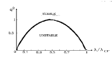
Figure 1: Toomre’s stability diagram for a thin stellar disc in the hydrodynamic approximation. The region of instability lies below the marginal curve. $Q$ is Toomre’s parameter, $\lambda=2\pi/k$, and $\lambda_{\rm cr}\equiv\lambda_{\rm T}.$

$L_{\rm corr}$ can also be identified with the spatial extent of the pattern since its inverse is the width of the spread in the wave number space, and the expression in parentheses on the left-hand side of Eq. (3), if equated to zero, yields Toomre’s dispersion relation for Lin’s spiral density waves in the approximation of collisionless hydrodynamics with $\omega-m\Omega=0$. This is the equation of the marginal curve shown in Fig. 1.

Now consider the response in the vicinity of the top point in Toomre’s diagram. Assuming $k=0$ in Eq. (4), i.e., $k^{*}=k_{\rm cr}=\pi G\sigma/c_{r}^{2}$, we obtain for the amplitude of a mode whose scale is close to the critical value $k_{\rm cr}^{-1}$:

$$\frac{\sigma_{m}}{\sigma}={{\psi_{1,\rm ext}\over{c^{2}_{r}}}\,{{c_{\rm T}^{2}}\over{c^{2}_{r}-c_{\rm T}^{2}}}}\;.$$ (5)

This yields the critical exponent as $\gamma=1$ for $c_{r}>c_{\rm T}$ from the definition $\sigma_{m}=\chi\psi_{1,\rm ext}$ of the susceptibility $\chi$ and the definition of $\gamma$, $\chi\sim(c_{r}^{2}-c_{\rm T}^{2})^{-\gamma}$. As expected, the correlation length is related to the susceptibility (Ma 1976, Patashinsky & Pokrovsky 1975). The spontaneous value of the order parameter $\sigma_{m}/\sigma$ in the post-critical state is also related to $L_{\rm corr}$ (Patashinsky & Pokrovsky 1975), i.e., is determined not only by the direct local correlation, but also by the global correlation chain whose scale grows as the critical point $c_{r}=c_{\rm T}$ is approached.

There are further implications of Eq. (4). For $c_{r}<c_{\rm T}$, this equation is inapplicable if $k$ tends to zero remaining on the marginal curve because then Fredholm’s alternative for the inhomogeneous problem is violated. Physically this means that matter motions in the disc must be allowed, for which nonlinear analysis would be required.

Two types of the critical behaviour of the disc can occur. Firstly, the disc can become dynamically unstable, leading to processes similar to those studied by theory of synergetics. Secondly, a phase transition can occur, similar to the gas–liquid phase transition at  a critical point. Here we investigate the latter posibility.

3 The order parameter, susceptibility and critical exponents in the critical and post-critical states

In the previous section and Appendix, the disc was treated in the linearized WKB approximation as an isothermal disc. In this section a different, non-linear expression for the ‘pressure’ perturbation must be used. The reason is that the properties of the disc matter change at $c_{r}=c_{\rm T}$. The disc has different properties in the pre-critical state ($c_{r}>c_{\rm T}$), in the marginal one ($c_{r}=c_{\rm T}$) and in the post-critical state ($c_{r}<c_{\rm T},\ |c_{r}-c_{\rm T}|<<c_{\rm T}$). In the latter state, the mean field $\psi_{1,{\rm int}}$ is no longer destroyed by the peculiar motions of the stars and, presumably, affects the disc properties. One can use the linear response function when $c_{r}>c_{\rm T}$ as in Section 2. However, the linear approximation (linear perturbation analysis) must be abandoned when we consider in this section the general equilibrium state for the marginal and post-critical regimes. We consider perturbations of a small, but finite amplitude.

Let us return to Eq. (2). As follows from the linear theory of density waves and from the above analysis, the most unstable (critical), as well as the most susceptible wave number is given by $k^{*}_{m,\rm uns}=2k_{\rm T}/Q^{2}$ in the marginal state with $\omega-m\Omega=0$ and $Q=1$, where $k_{T}=\kappa^{2}/(2\pi G\sigma),$ $Q=c_{r}/c_{\rm T},$ and $c_{\rm T}=(\pi G\sigma)/\kappa$ (see Fig. 1). For this mode, Eq. (2) takes the form

$$\frac{\sigma_{m}}{\sigma}\kappa^{2}=(-c^{2}_{r}k_{m,\rm uns}^{*2}+2\pi G\sigma|k_{m,\rm uns}^{*}|)\frac{\sigma_{m}}{\sigma}+\psi_{1,\rm ext}k_{m,\rm uns}^{*2}\;.$$ (6)

Using $k_{m,\rm uns}=\kappa/c_{\rm T}$, canceling $\kappa^{2}$ and after some algebra, Eq. (6) can be reduced to

$$\frac{\sigma_{m}}{\sigma}(c^{2}_{r}-c_{\rm T}^{2})=\psi_{1,\rm ext}\;.$$ (7)

Equation (7) correctly describes the susceptibility of the critical mode for $c_{r}>c_{\rm T}$ but does not yield spontaneous phase transition (at $\psi_{1,\rm ext}=0$). Furthermore, it does not describe the susceptibility in the post-critical state $c_{r}<c_{\rm T}$ since it has been obtained without taking into account changes in the disc’s state.

Now we leave the mode analysis for the general equilibrium relations. We recall that in fact a stellar disc is a collisionless dynamic system.

The relation between ‘pressure’ perturbation $\Delta p$ and gravitational potential function $\psi_{1}$ applicable to static perturbations over half the Toomre wavelength (i.e., the critical scale) has the form

$${\Delta p\over\sigma}-\psi_{1}=0\;.$$ (8)

Such perturbations can be called frozen. They satisfy the general hydrostatic equilibrium equation for a system in an external field known from statistical physics (Landau & Lifshitz 1976, §25):

$$\mu_{0}(P,T)-\Psi(\bf{r})={const}\;,$$

where $\mu_{0}$ and $\Psi$ are the specific chemical potential (without the field) and field potential, respectively, $P$ is the ‘pressure’, and $T$ is the temperature of the system. $\Psi$ is reduced by the centrifugal potential (cf. Eq. (23) of the Appendix A that describes hydrostatic equilibrium of the disc in the pre-critical state).

The ‘pressure’ perturbation near  the  critical  point (i.e.,  the  top of Toomre’s diagram) can be written in a form similar to that used by Landau in his theory of van der Waals’ critical point (Landau & Lifshitz 1976, §152):

$${\Delta p\over\sigma}=c^{2}_{r}{\sigma_{m}\over\sigma}+4c^{2}_{\rm T}{\sigma^{3}_{m}\over\sigma^{3}}\;.$$ (9)

The applicability of this expression to stellar discs is our assumption, justified a posteriori by the results obtained. This expression follows from general arguments presented, e.g., by Landau & Lifshitz (1976, §§144, 152). For static perturbations, this expression results in one real and two imaginary solutions for $\sigma_{m}$ when $c_{r}>c_{\rm T}$ and three real solutions when $c_{r}<c_{\rm T}$. Thus, the expression (9) leads to a reasonable physical behaviour similar to that of a gas–liquid system, in the sense that the stellar disc maintains hydrostatic equilibrium near its marginal state. The expression (9) simply implies the expansion of $\Delta p$ in power of $\sigma_{m}$, supposing the inflection (bending) point for equation of state function of a stellar disk $p(\sigma)$ (in a marginal state), as $\Delta p=(dp/d\sigma)\sigma_{m}+(1/n!)(d^{3}p/d\sigma^{3})\sigma_{m}^{3}$. That is, the disc’s state is assumed to change as the disc passes through the critical point, as we pointed out in Abstract, the inflection (bending) point is appeared .

The term nonlinear in $\sigma_{m}$ in the expression (9) can be understood in the followimg semi-quantitative way. A density perturbation $\sigma_{m}$ leads to an increase in stellar velocities on their orbits by $\Delta v$ due to an increase in the gravitational force. For static perturbations, the velocity incerement can be found from centrifugal balance as $\Omega\Delta v=\pi G\sigma_{m}.$ Thus, $\Delta v=\pi G\sigma_{m}/\Omega\approx 2\pi G\sigma_{m}/\kappa$. The resulting ‘pressure’ increment $\Delta p$ is given by ${(\Delta v)}^{2}\sigma_{m}\approx 4(\pi G\sigma/\kappa)^{2}(\sigma_{m}/\sigma)^{2}\sigma_{m}$, which is just the nonlinear term of the expression (9). This term represents an additional ‘elasticity’ (apart from that of the epicyclic motion, represented by $c_{r}$) that arises from the stability of the circular orbits, associated with the centrifugal force, because the orbits are assumed to sustain gravitational perturbations for $c_{r}\leq c_{\rm T}$.

We note that

$$\psi_{1} = \psi_{1,\rm int}+\psi_{1,\rm ext}\;,$$

$$\psi_{1,\rm int} = \pi G\sigma_{m}r_{\rm corr}=\pi G\sigma_{m}{c_{\rm T}\over\kappa}=c_{\rm T}^{2}{\sigma_{m}\over\sigma}\;,$$

which results, using Eq. (8), in the following equation for the order parameter $\sigma_{m}$:

$$\frac{\sigma_{m}}{\sigma}\left[c^{2}_{r}-c_{\rm T}^{2}+4c_{\rm T}^{2}\left(\frac{\sigma_{m}}{\sigma}\right)^{2}\right]=\psi_{1,\rm ext}\;.$$ (10)

Equation (10) has a standard form for an equation describing phase equilibrium in Landau’s theory of the phase transition of the second kind (Landau & Lifshitz 1976). This equation yields the ratio controlling the susceptibility $\partial\sigma_{m}/\partial\psi_{1,\rm ext}$ in the pre-critical state ($c_{r}>c_{\rm T}$),

$$\frac{\partial\sigma_{m}}{\partial\psi_{1,\rm ext}}=\chi=\frac{\sigma}{c^{2}_{r}-c^{2}_{\rm T}}\;,$$ (11)

together with expressions for the dependence of the order parameter on $c^{2}_{r}-c^{2}_{\rm T}$ (if evaluated at $\psi_{1,\rm ext}=0$, see Eq. (12) below) and on the external field (if evaluated at $c_{r}=c_{\rm T}$; note that the result remains non-singular),

$$\sigma_{m}\sim\psi_{1,\rm ext}^{1/\delta}\;.$$

Thus, there are three critical exponents, $\gamma=1,\ \beta=1/2$ and $\delta=3.$ These are not independent but related by Widom’s ratio (Landau & Lifshitz 1976, §148), $\beta\delta=\beta+\gamma$.

For $c_{r}<c_{\rm T}$, the susceptibility has to be found for a non-zero value of $\sigma_{m}$. For this purpose the bracket in Eq. (10) should be put equal to zero. For $c_{r}<c_{\rm T}$ we obtain a real solution of the type $\sigma_{m}/\sigma\sim{(c_{\rm T}^{2}-c_{r}^{2})}^{\beta}$ which is given by

$$\left({\sigma_{m}\over{\sigma}}\right)^{2}=-{{c_{r}^{2}-c_{\rm T}^{2}}\over{4c_{\rm T}^{2}}}\;.$$ (12)

For $c_{r}>c_{\rm T}$, Eq. (12) formally gives purely imaginary density perturbations, implying that static density perturbations of finite amplitude cannot exist in this case.

Differentiating Eq. (10) and using Eq. (12), we find the susceptibility in the post-critical case as

$$\frac{\partial\sigma_{m}}{\partial\psi_{1,\rm ext}}=\chi = \frac{\sigma}{c_{r}^{2}-c_{\rm T}^{2}+12c_{\rm T}^{2}(\sigma_{m}/\sigma)^{2}}$$ (13)

$$= -{\sigma\over 2(c_{r}^{2}-c_{\rm T}^{2})}\;.$$

Comparing Eqs (11) and (13), we see that the susceptibility suffers a jump at $c_{r}=c_{\rm T}$ as it should at a phase transition.

Finally, the exponents follow as $\beta=1/2,\ \gamma=1,\ \delta=3,$ and $\nu=1/2.$ The scalings of Eqs (11)–(13) agree with the results of Landau–Weiss’s standard theory (Landau & Lifshitz 1976).

4 Conclusions

In the spirit of Landau’s theory of the van der Waals critical point and the generic nature of critical phenomena, we have shown the possibility of critical behaviour of galactic stellar discs. The disc undergoes a phase transition when the stellar velocity dispersion $c_{r}$ is equal to Toomre’s critical value, $c_{\rm T}$. It appears that the transition leads to the formation of a fundamental spiral structure. We have shown that well-known features of such phase transitions result in an essentially new mechanism for the spiral structure formation. Similarly to a thermodynamic system undergoing the gas–liquid phase transition at a critical point, a marginally stable collisionless stellar disc can, while retaining (or tending to retain) its hydrostatic equilibrium, exhibit a critical behaviour that leads to its primary spatial inhomogeneity which can further develop into a spiral structure. This is the main point of our approach which takes advantage of the theory of critical phenomena; linear results are a part of our analysis, but they are not sufficient for it.

Numerical experiments of Hohl (1975, 1975a) demonstrate that a stellar disc embedded in a bulky halo appears to be rather changeable at $Q=Q_{\rm cr}$. Processes different from the bar instability ‘thermalize’ the disc quickly (practically instantaneously), heating it up to $Q\approx(2$–$3)Q_{\rm cr}$. At the initial stage of the process, the disc is populated by a set of stellar splinters and crescents, and a few large-scale spiral branches develop later. These structures eventually reduce to decaying worm-type features because of the ‘heating’ most likely resulting from the instability of individual stellar orbits due to resonances. This demonstrates that both dynamical instabilities and fluctuations (critical and, for example, induced by embedding bulky masses) can be superimposed on the process wherein an order emerges. This scenario is also confirmed by numerical calculations of critical dynamics in a model one-dimensional self-gravitating system in a marginal state (Ivanov 1992, 1993).

‘Hot’ discs cannot have quasistatic structures, and this fact corroborates our theory of phase transitions. Our theory is only applicable to early stages of the simulations discussed above before instabilities have developed. There are many effects that can halt the ordering process, so it can occur only in some galaxies.

We have considered only compressional perturbations. But the last term in the expression (9) for $\Delta p/\sigma$ can be compared with a change in the stellar velocity driven by gravitational perturbations during the phase transition, namely with the drift correction to the chaotic stellar velocity, whose azimuthal component is given by $|\kappa^{-1}\partial\psi_{1,\rm int}/\partial r|$ and the radial component by $|(\kappa r)^{-1}\partial\psi_{1,\rm int}/\partial\varphi|$ (Ivannikova & Maksumov 1994). The square of the drift correction to the velocity is given by $|\kappa^{-1}\partial\psi_{1,\rm int}/\partial r|^{2}+|(\kappa r)^{-1}\partial\psi_{1,\rm int}/\partial\varphi|^{2}$. Using $\psi_{1,\rm int}=2\pi G\sigma_{m}/|k^{*}|$, $k^{*}_{m,\rm uns}=\kappa/c_{\rm T}$, $|\kappa^{-1}\partial\psi_{1,\rm int}/\partial r|=2c_{\rm T}(\sigma_{m}/\sigma)\cos\delta$ and $(\kappa r)^{-1}\partial\psi_{1,\rm int}/\partial\varphi|=2c_{\rm T}(\sigma_{m}/\sigma)\sin\delta$, the drift correction squared can be expressed as $4c_{\rm T}^{2}(\sigma_{m}/\sigma)^{2}.$ This estimates confirms the possibility of translational and shearing effects in addition to the compressional one.

5 Appendix A: The derivation of Eq. (1) for density perturbations in a stellar disc. The drift perturbations

Linearized hydrodynamic equations for the density perturbation $\sigma_{m}$ and the radial and azimuthal bulk velocities $u$ and $v$ are given by (Rohlfs 1977, §5.5)

$$\frac{\partial\sigma_{m}}{\partial t}+\Omega\frac{\partial\sigma_{m}}{\partial\varphi}+\frac{1}{r}\left[\frac{\partial}{\partial r}(r\sigma u)+\frac{\partial}{\partial\varphi}(\sigma v)\right]=0\;,$$ (14)

$$\frac{\partial u}{\partial t}+\Omega\frac{\partial u}{\partial\varphi}-2\Omega v=-\frac{c^{2}_{r}}{\sigma}\,\frac{\partial\sigma_{m}}{\partial r}+\frac{\partial\psi_{1}}{\partial r}\;,$$ (15)

$$\frac{\partial v}{\partial t}+\Omega\frac{\partial v}{\partial\varphi}+\frac{\kappa^{2}}{2\Omega}u=-\frac{1}{r}\left(\frac{c^{2}_{\varphi}}{\sigma}\,\frac{\partial\sigma_{m}}{\partial\varphi}-\frac{\partial\psi_{1}}{\partial\varphi}\right).$$ (16)

Assuming that the perturbed quantities (including $\psi_{1}$) are proportional to $\exp[i(\omega t-m\varphi+kr)]$ and reserving for amplitudes the notation used for the respective perturbed quantities, we transform these equations first similarly to Lin & Shu (1964) who considered tightly wound perturbations. Equations (14), (15) and (16) reduce to

$$i(\omega-m\Omega)\sigma_{m}+i\sigma ku+{d\sigma\over dr}u-i\sigma k_{\varphi}v=0\;,$$ (17)

$$i\frac{kc^{2}_{r}}{\sigma}\sigma_{m}+i(\omega-m\Omega)u-2\Omega v=ik\psi_{1}\;,$$ (18)

$$i(\omega-m\Omega)v+\frac{\kappa^{2}}{2\Omega}u=i\frac{k_{\varphi}c^{2}_{\varphi}}{\sigma}\sigma_{m}-ik_{\varphi}\psi_{1}\;.$$ (19)

Equation (19) yields for $v$:

$$v=i\frac{\kappa^{2}}{2\Omega(\omega-m\Omega)}u+\frac{k_{\varphi}c^{2}_{\varphi}\sigma_{m}/\sigma-k_{\varphi}\psi_{1}}{\omega-m\Omega}\;.$$

Using this expression in Eq. (18), we find $u$ and $v$ as

$$u = {{\omega-m\Omega}\over{{(\omega-m\Omega)}^{2}-\kappa^{2}}}$$

$$\mbox{}\!\!\times\!\left[-k\left(c^{2}_{r}{\sigma_{m}\over\sigma}-\psi_{1}\right)-\frac{2i\Omega}{\omega-m\Omega}k_{\varphi}\left(c^{2}_{\varphi}\frac{\sigma_{m}}{\sigma}-\psi_{1}\right)\right];$$

$$v = {{i\kappa^{2}/2\Omega}\over{{(\omega-m\Omega)}^{2}-\kappa^{2}}}$$

$$\mbox{}\!\!\times\!\left[-k\left(c^{2}_{r}{\sigma_{m}\over\sigma}-\psi_{1}\right)-i{2\Omega\over{\omega-m\Omega}}k_{\varphi}\left(c^{2}_{\varphi}{\sigma_{m}\over\sigma}-\psi_{1}\right)\right]$$

$$\mbox{}+{k_{\varphi}\over{\omega-m\Omega}}\left(c^{2}_{\varphi}{\sigma_{m}\over\sigma}-\psi_{1}\right).$$

Using $c^{2}_{\varphi}=(\kappa^{2}/2\Omega)c^{2}_{r}$, we find from Eq. (17):

$$\frac{\sigma_{m}}{\sigma} = \frac{1}{[(\omega-m\Omega)^{2}-\kappa^{2}](\omega-m\Omega)^{2}}$$

$$\mbox{}\times\left[(k^{2}+k_{\varphi}^{2})(\omega-m\Omega)^{2}\left(c^{2}_{r}\frac{\sigma_{m}}{\sigma}-\psi_{1}\right)\right.$$

$$\mbox{}+k_{\varphi}^{2}(\omega-m\Omega)^{2}c_{r}^{2}\,\frac{1}{2}\,\frac{d\ln\Omega}{d\ln r}\,\frac{\sigma_{m}}{\sigma}$$

$$\mbox{}+2\Omega(\omega-m\Omega)\frac{d\ln\sigma}{dr}k_{\varphi}\left(\frac{\kappa^{2}}{2\Omega}\,c^{2}_{r}\,\frac{\sigma_{m}}{\sigma}-\psi_{1}\right)$$

$$\mbox{}+ikk_{\varphi}(\omega-m\Omega)\,r\frac{d\Omega}{dr}\,\psi_{1}$$

$$\mbox{}\left.-i(\omega-m\Omega)^{2}\,\frac{d\ln\sigma}{dr}\,k\left(c^{2}_{r}\frac{\sigma_{m}}{\sigma}-\psi_{1}\right)\right].$$

Neglecting terms with spatial derivatives of $\sigma$ and $\Omega$, we obtain Eq. (1).

Now consider slow, drift modes. They are basically different from the tightly wound ones and can only be nonaxisymmetric. Their susceptibility is easier to consider in the limit $\partial/\partial t+\Omega\partial/\partial\varphi=0$. The system (14)–(16) then takes the form

$$\frac{\partial}{\partial r}(r\sigma u)+\frac{\partial}{\partial\varphi}(\sigma v)=0\;,$$ (20)

$$2\Omega v=\frac{c^{2}_{r}}{\sigma}\,\frac{\partial\sigma_{m}}{\partial r}-\frac{\partial\psi_{1}}{\partial r}\;,$$ (21)

$$\frac{\kappa^{2}}{2\Omega}\,u=-\frac{1}{r}\left(\frac{c^{2}_{r}}{\sigma}\,\frac{\partial\sigma_{m}}{\partial\varphi}-\frac{\partial\psi_{1}}{\partial\varphi}\right).$$ (22)

In the limit $u,v\to 0$ we obtain an expression used to determine the susceptibility of the drift modes:

$$c^{2}_{r}\,\frac{\sigma_{m}}{\sigma}-\psi_{1}=0\;.$$ (23)

Using $\psi_{1}=\psi_{1,\rm int}+\psi_{1,\rm ext}$ and $\psi_{1,\rm int}=2\pi G\sigma_{m}/|k^{*}|$ with $k^{*}=4k_{\rm T}$, $k^{*}={(k^{2}+k_{\varphi}^{2})}^{1/2}$, we obtain Eq. (11) for the susceptibility $\chi$.

References

- [1] Balescu R., 1975, Equilibrium and nonequilibrium statistical mechanics. Wiley , N. Y., Ch. 9 and 10
- [2] Hohl F., 1975, in Weliachew L., ed., La dynamique des galaxies spirales. Coll. Intern. du CNRS, 16–20 septembre 1974. Paris, p. 55
- [3] Hohl F., 1975a, in Hayli A., ed., Dynamics of Stellar Systems. IAU Symp. 69. Kluwer, Dordrecht, p. 349
- [4] Ivannikova E. I., Ivanov A. V., Maksumov M. N., 1994, in Astrophysics and Cosmology after Gamov. Abstract Book. Kosmoinform, Moscow, p. 18
- [5] Ivannikova E. I., Ivanov A. V., Maksumov M. N., 1997, in Agekian T. A., T. A. Mülläri, V. V. Orlov, eds, Structure and Evolution of Stellar Systems. St. Petersburg Univ. Press, St. Petersburg, p. 271
- [6] Ivannikova E. I., Maksumov M. N., 1994, AZh, 71, 216
- [7] Ivanov A. V., 1992, MNRAS, 259, 576
- [8] Ivanov A. V., 1993, Vistas Astron., 37, 543
- [9] Landau L. D., Lifshitz E. M., 1976, Statistical physics, Pt. 1. Nauka, Moscow (in Russian)
- [10] Lin C. C., Shu F. H., 1964, ApJ, 140, 646
- [11] Ma Sh.-K., 1976, Modern Theory of Critical Phenomena. Benjamin, London
- [12] Patashinsky A. Z., V.L.Pokrovsky V.L., Fluctuational Theory of Phase Transitions. Nauka, Moscow (in Russian), §4 of Ch. 1 and §1 of Ch. 2
- [13] Rohlfs K., 1977, Lectures on Density Wave Theory. Springer, Berlin
- [14] Saslaw W. C., 1987, Gravitational Physics of Stellar and Galactic Systems. Cambridge Univ. Press, Cambridge
- [15] Toomre A., 1964, ApJ, 139, 1217