Testable dark energy predictions from current data

Abstract

Given a class of dark energy models, constraints from one set of cosmic acceleration observables make predictions for other observables. Here we present the allowed ranges for the expansion rate $H(z)$, distances $D(z)$, and the linear growth function $G(z)$ (as well as other, derived growth observables) from the current combination of cosmological measurements of supernovae, the cosmic microwave background, baryon acoustic oscillations, and the Hubble constant. With a cosmological constant as the dark energy and assuming near-minimal neutrino masses, the growth function is already predicted to better than $2\%$ precision at any redshift, with or without spatial curvature. Direct measurements of growth that match this precision offer the opportunity to stringently test and potentially rule out a cosmological constant. While predictions in the broader class of quintessence models are weaker, it is remarkable that they are typically within a factor of $2-3$ of forecasts for future space-based supernovae and Planck CMB measurements. In particular, measurements of growth at any redshift, or the Hubble constant $H_{0}$, that exceed $\Lambda$CDM predictions by substantially more than $2\%$ would rule out not only a cosmological constant but also the whole quintessence class, with or without curvature and early dark energy. Barring additional systematic errors hiding in the data, such a discovery would require more exotic explanations of cosmic acceleration such as phantom dark energy, dark energy clustering, or modifications of gravity.

I Introduction

Within a fixed class of dark energy models, such as the cosmological constant or scalar field quintessence, various cosmological observables are all interrelated by the properties of the class itself. The narrower the class, the higher the expected correlation between measurements of different observables. Therefore, given a class of dark energy models, constraints from one set of cosmic acceleration observables make predictions for other observables. For example, it is well known that since the first release of WMAP data Spergel_2003 , the Hubble constant in a spatially flat universe with a cosmological constant and cold dark matter ($\Lambda$CDM) has been predicted to a precision better than it has yet been measured. Predictions like this one therefore offer the opportunity for more precise measurements to falsify the dark energy model (in this case, flat $\Lambda$CDM) Hu_standards .

In a previous paper (hereafter MHH) PaperI , we showed how this idea can be generalized to additional acceleration observables and wider classes of dark energy models. Other observables include the expansion rate $H(z)$, the comoving angular diameter distance $D(z)$, and the linear growth function $G(z)$. The model classes we considered include a cosmological constant, with and without spatial curvature, and scalar field quintessence models, with and without early dark energy and spatial curvature components. Using forecasts for a Stage IV DETF SN sample and Planck CMB data, we found that future data sets will provide numerous strong predictions that we may use to attempt to falsify various acceleration paradigms.

In this paper, we evaluate the predictive power of current measurements to constrain the expansion rate, distance, and growth as a function of redshift. Specifically, we consider current measurements of supernovae (SN), the cosmic microwave background (CMB), baryon acoustic oscillations (BAO), and the Hubble constant ($H_{0}$). These predictions target the redshift ranges and required precision for future measurements seeking to rule out whole classes of models for cosmic acceleration.

Our approach complements studies that seek to constrain an ever expanding set of parameters of the dark energy. The most ambitious analyses currently utilize $\sim 5$ parameters to describe the dark energy equation of state $w(z)$ Huterer_Cooray ; Wang_Tegmark_2005 ; Riess_2006 ; Zunckel_Trotta ; Sullivan_Cooray_Holz ; Zhao_Huterer_Zhang ; Zhao_Zhang:2009 ; Serra:2009 . We take these studies in a new direction: rather than constraining parameters associated with the equation of state, we propagate constraints from the data into allowed ranges for $H(z)$, $D(z)$, $G(z)$, and auxiliary observables that can be constructed from them through a principal component representation of $w(z)$ that is complete in these observables for $z<1.7$. This work goes beyond previous studies that are similar in spirit (e.g. Kujat ; Sahlen05 ; Huterer_Peiris ; Chongchitnan_Efstathiou ; ZhaKnoTys08 ) by directly applying constraints from current data sets to complete representations of several dark energy model classes and making concrete predictions for a number of observable quantities.

This paper is organized as follows. We begin in Sec. II with a discussion of the methodology of predicting observables within classes of dark energy models, including descriptions of each of the acceleration observables, cosmological data sets, and model classes. We present our predictions from current data in Sec. III and discuss the results in Sec. IV.

II Methodology

II.1 Acceleration Observables

There are two general types of acceleration observables: those related to the expansion history and geometry of the universe, and those related to the growth of structure. In terms of a general evolution for the dark energy equation of state $w(z)$, the expansion history observables are the Hubble expansion rate

$$H(z) = H_{0}\left[\Omega_{\rm m}(1+z)^{3}+\Omega_{\rm DE}f(z)+\Omega_{\rm K}(1+z)^{2}\right]^{1/2},$$ (1)

$$f(z)=\exp\left[3\int_{0}^{z}dz^{\prime}\frac{1+w(z^{\prime})}{1+z^{\prime}}\right],$$

where $\Omega_{\rm m}$ and $\Omega_{\rm DE}$ are the present matter and dark energy densities, respectively, as fractions of the critical density for flatness, spatial curvature is parametrized by $\Omega_{\rm K}\equiv 1-\Omega_{\rm m}-\Omega_{\rm DE}$, and the small contribution of radiation at $z\sim 1$ is neglected; and the comoving angular diameter distance

$$D(z)=\frac{1}{(|\Omega_{\rm K}|H_{0}^{2})^{1/2}}S_{\rm K}\left[(|\Omega_{\rm K}|H_{0}^{2})^{1/2}\int_{0}^{z}\frac{dz^{\prime}}{H(z^{\prime})}\right],$$ (2)

where the function $S_{\rm K}(x)$ is equal to $x$ in a flat universe ($\Omega_{\rm K}=0$), $\sinh x$ in an open universe ($\Omega_{\rm K}>0$), and $\sin x$ in a closed universe ($\Omega_{\rm K}<0$). The growth of linear density perturbations $\delta\propto Ga$ is given by

$$G^{\prime\prime}+\left(4+\frac{H^{\prime}}{H}\right)G^{\prime}+\left[3+\frac{H^{\prime}}{H}-\frac{3}{2}\Omega_{\rm m}(z)\right]G=0,$$ (3)

where primes denote derivatives with respect to $\ln a$ and $\Omega_{\rm m}(z)=\Omega_{\rm m}H_{0}^{2}(1+z)^{3}/H^{2}(z)$. We assume scales for which the dark energy density is spatially smooth compared with the matter and normalize $G(z)=1$ at $z=10^{3}$.

There are several auxiliary quantities related to the growth function that are also interesting to examine. Since growth measurements like the evolution of the cluster abundance often compare the change in growth relative to the present, we also consider a different normalization for the growth function,

$$G_{0}(z)\equiv\frac{G(z)}{G(0)}.$$ (4)

Velocity field measurements, on the other hand, are sensitive to the growth rate

$$f(z)\equiv 1+\frac{G^{\prime}}{G}.$$ (5)

Specifically, the amplitude of the velocity power spectrum can be measured from redshift space distortions and constrains $f(z)G(z)$ independently of galaxy bias (e.g. see Percival_White ). Finally, given that the growth rate is approximately related to expansion history observables by $f(z)=[\Omega_{\rm m}(z)]^{\gamma}$ where the growth index is $\gamma\approx 0.55$ for flat $\Lambda$CDM WangSteinhardt ; Linder_gamma we also consider predictions for

$$\gamma(z)\equiv{\ln[f(z)]\over\ln[\Omega_{\rm m}(z)]}\,.$$ (6)

Note however that $\gamma(z)$ is not a direct observable but rather must be inferred from a combination of measurements in a specific dark energy context.

We ignore the influence of massive neutrinos throughout this study. The effect of massive neutrinos on the growth of structure is significantly scale-dependent, but on present linear scales well below the horizon, $k\sim 0.01-0.1~{}h$ Mpc^-1, the growth suppression from a normal neutrino mass hierarchy with $\sum m_{\nu}\sim 0.05$ eV nu_oscill is $\lesssim 1\%$ in $G(z)$ and $f(z)G(z)$ and smaller for other observables. The maximum decrement in growth from nearly-degenerate neutrinos with $\sum m_{\nu}\sim 0.5$ eV (e.g. Reid_SDSSDR7 ) is $\sim 1-10\%$ on these scales. In the predictions we present here, these effects would appear as an additional “early” dark energy component with $w\approx 0$. Future precise measurements of $\sum m_{\nu}$ from independent data could be used to correct the growth predictions here by scaling them by the appropriate suppression factor.

II.2 Constraints from Current Data

The main observational constraints we consider when making predictions for acceleration observables include relative distances at $z\lesssim 1.5$ from Type Ia SNe and absolute distances at $z_{*}=1090$ from the CMB, $z_{\rm BAO}\approx 0.35$ from BAO, and $z_{h}\approx 0.04$ from low-redshift SNe calibrated with maser and Cepheid distances. Since low-$z$ distances mainly probe the Hubble constant for smoothly varying $w(z)$, we refer to the low-$z$ SN calibration as an $H_{0}$ constraint. The CMB data additionally constrain parameters that impact dark energy models such as the matter density $\Omega_{\rm m}h^{2}$ and the fraction of dark energy density at recombination.

In the simplest classes of models, the SN and CMB data suffice to make accurate predictions for expansion and growth observables. In more complex classes, BAO and $H_{0}$ constraints on distances are necessary. Even in these cases, predictive power is still retained in that measured distances to a few specific redshifts constrain $H(z)$, $D(z)$, and $G(z)$ at all redshifts. We now describe each of these data sets in more detail.

The Type Ia SN sample we use is the Union compilation SCP_Union . These SN observations measure relative distances, $D(z_{1})/D(z_{2})$, over a range of redshifts spanning $0.015\leq z\leq 1.551$, with most SNe at $z\lesssim 1$. We add the SN constraints using the likelihood code for the Union data sets Union_like , which includes estimated systematic errors for the SN data SCP_Union .

For the CMB, we use the most recent, 5-year release of data from the WMAP satellite Komatsu_2008 ; Nolta_2008 ; Dunkley_2008 employing the likelihood code available at the LAMBDA web site WMAP_like . Unlike the CMB distance priors on $D(z_{*})$ and $\Omega_{\rm m}h^{2}$ used for the forecasts in MHH, the likelihood used here contains the full information from the CMB angular power spectra; in particular this provides sensitivity to large fractions of early dark energy at recombination as well as information about late-time dark energy and spatial curvature from the ISW effect without necessitating additional priors. We compute the CMB angular power spectra using the code CAMB Lewis:1999bs ; camb_url modified with the parametrized post-Friedmann (PPF) dark energy module PPF ; ppf_url to include models with general dark energy equation of state evolution where $w(z)$ may cross $w=-1$. Note that while our predictions for growth observables apply to scales on which dark energy is smooth relative to matter, the CAMB+PPF code self-consistently accounts for the effects of scale-dependent dark energy perturbations on the CMB anisotropies.

The BAO constraint we use is based on the measurement of the correlation function of SDSS Luminous Red Galaxies (LRGs) Eisenstein , which determines the distance and expansion rate at $z_{\rm BAO}\approx 0.35$ through the combination $D_{V}(z)\equiv[zD^{2}(z)/H(z)]^{1/3}$. We implement this constraint by taking the volume average of this quantity, $\langle D_{V}\rangle$, over the LRG redshifts, $0.16<z<0.47$, and comparing with the value of $A\equiv\langle D_{V}\rangle\sqrt{\Omega_{\rm m}h^{2}}/z_{\rm BAO}$ given in Ref. Eisenstein , $A=0.472\pm 0.017$ (taking the scalar spectral tilt to be $n_{s}=0.96$). We discuss the expected impact of more recent BAO measurements Percival09 on our predictions in Sec. IV.

Finally, we include the recent Hubble constant constraint from the SHOES team SHOES , based on SN distances at $0.023<z<0.1$ that are linked to a maser-determined absolute distance using Cepheids observed in both the maser galaxy and nearby galaxies hosting Type Ia SNe. The SHOES measurement determines the absolute distance to a mean SN redshift of $z_{h}=0.04$, which effectively corresponds to a constraint on $H_{0}$ for models with relatively smooth dark energy evolution in the recent past such that $\lim_{z\to 0}D(z)=cz/H_{0}$. Sharp transitions in the dark energy density at ultra-low redshifts can break the relationship between low-redshift distances and $H_{0}$ as described in Ref. HubTrans , but the principal component parametrization we use is constructed to largely eliminate such possibilities (see MHH, Appendix B). Nonetheless, given that the observations relate distance and redshift, and distances are more robust to variations in the equation of state at low redshift than is the instantaneous expansion rate, we implement the $H_{0}$ constraint as a measurement of $D(z_{h})=cz_{h}/(74.2\pm 3.6$ km s^-1 Mpc^-1).

II.3 Model Classes

Our basic model classes are (1) “$\Lambda$CDM,” where dark energy is a cosmological constant $\Lambda$ with equation of state $w=-1$, and (2) “quintessence,” the general class of scalar field models with arbitrary but bounded equation of state evolution $-1\leq w(z)\leq 1$. For these two cases we maintain a complete description of the observable degrees of freedom. Finally, there is (3) “smooth dark energy” which is the generalization of quintessence to unbounded $w(z)$, assuming that dark energy is unclustered relative to matter. Unlike the forecasts in MHH, we do not maintain completeness for smooth dark energy but rather take a fixed functional form $w(z)=w_{0}+(1-a)w_{a}$. This choice allows us to simply identify observables that could potentially falsify quintessence in favor of smooth dark energy but does not allow us to make predictions that could falsify the broader class as a whole. It also allows us to identify how predictions in the quintessence class change if we require smooth, monotonic evolution in $w(z)$. In each case, the model class can either be restricted to spatially flat cosmologies or allow spatial curvature, parametrized by $\Omega_{\rm K}$

Table 1: Dark energy model classes, their defining parameter sets and priors, and figures in which predictions appear.

Model Class	Parameters	Priors	Figures
flat $\Lambda$CDM	$\bm{\theta}_{\Lambda}$	$\Omega_{\rm K}=0$	1, 2, 3, 8
non-flat $\Lambda$CDM	$\bm{\theta}_{\Lambda}$	none	2
flat PC quintessence without early dark energy	$\bm{\theta}_{\rm Q}$	$\{\alpha_{i}\}$ priors, $\Omega_{\rm K}=0$, $w_{\infty}=-1$	3, 4, 5, 6, 8
flat PC quintessence with early dark energy	$\bm{\theta}_{\rm Q}$	$\{\alpha_{i}\}$ priors, $\Omega_{\rm K}=0$	5
non-flat PC quintessence without early dark energy	$\bm{\theta}_{\rm Q}$	$\{\alpha_{i}\}$ priors, $w_{\infty}=-1$	6, 7
non-flat PC quintessence with early dark energy	$\bm{\theta}_{\rm Q}$	$\{\alpha_{i}\}$ priors	7, 8
flat $w_{0}-w_{a}$ with quintessence priors	$\bm{\theta}_{\rm S}$	$-1\leq w_{0}\leq 1$, $-1\leq w_{0}+w_{a}\leq 1$, $\Omega_{\rm K}=0$	9
non-flat $w_{0}-w_{a}$ with quintessence priors	$\bm{\theta}_{\rm S}$	$-1\leq w_{0}\leq 1$, $-1\leq w_{0}+w_{a}\leq 1$	10
flat $w_{0}-w_{a}$ (no $w$ prior; smooth dark energy)	$\bm{\theta}_{\rm S}$	$\Omega_{\rm K}=0$	9
non-flat $w_{0}-w_{a}$ (no $w$ prior; smooth dark energy)	$\bm{\theta}_{\rm S}$	none	10

For the quintessence class, we follow the procedure described in MHH and parametrize $w(z)$ at $z<z_{\rm max}=1.7$ with a basis of principal components (PCs) Hu_PC ; Huterer_Starkman . For our purposes, the PCs simply act as an intermediate basis to represent observables, required to be complete for arbitrary variations in $w(z)$ at $z<z_{\rm max}$. We construct the PCs using the specifications of a Stage IV SN experiment, specifically the SuperNova/Acceleration Probe (SNAP) SNAP , combined with CMB information from the recently launched Planck satellite.

Specifically, the principal component functions $e_{i}(z_{j})$ are eigenvectors of the SNAP+Planck covariance matrix for the equation of state in redshift bins $z_{j}$, and they form a basis in which an arbitrary function $w(z_{j})$ may be expressed as

$$w(z_{j})-w_{\rm fid}(z_{j})=\sum_{i=1}^{N_{z,{\rm PC}}}\alpha_{i}e_{i}(z_{j}),$$ (7)

where $\alpha_{i}$ are the PC amplitudes, $N_{z,{\rm PC}}=1+z_{\rm max}/\Delta z$ is the number of redshift bins of width $\Delta z$, and $z_{j}=(j-1)\Delta z$. The maximum redshift for variations in $w(z)$ ($z_{\rm max}=1.7$) matches the largest redshift for the SNAP supernova data, and we use a fiducial model $w_{\rm fid}(z)=-1$ since $\Lambda$CDM is an excellent fit to current data.

Since the highest-variance PCs correspond to modes of $w(z)$ to which both data and predicted observables are insensitive, we truncate the sum in Eq. (7) with $N_{\rm max}<N_{z,{\rm PC}}$ PCs. As shown in MHH, for our choices of $z_{\rm max}$ and $w_{\rm fid}(z)$, the 10 lowest-variance PCs ($N_{\rm max}=10$) form a basis which, for the classes of models we consider here, is sufficiently complete for future Stage IV measurements and so more than suffice for the current data. We have also explicitly checked that there is little difference in predictions between $N_{\rm max}=5$ and $N_{\rm max}=10$ for one of the model classes, flat quintessence without early dark energy.

Quintessence models describe dark energy as a scalar field with kinetic and potential contributions to energy and pressure. Barring models where large kinetic and (negative) potential contributions cancel, quintessence equations of state are restricted to $-1\leq w(z)\leq 1$. Following MHH, this bound is conservatively implemented with uncorrelated top-hat priors on the PC amplitudes $\alpha_{i}$. Any combination of PC amplitudes that is rejected by these priors must arise from an equation of state $w(z)$ that violates the bound on $w(z)$, but not all models that are allowed by the priors strictly satisfy this bound; the set of models we consider is therefore “complete” but not “pure.” This ambiguity arises since we truncate the principal components at $N_{\rm max}=10$ and we wish to allow for the possibility that the omitted components may conspire to satisfy the bound. For the purposes of falsifying dark energy model classes a complete but impure sampling of quintessence models is sufficient, although more efficient rejection of models that violate the $-1\leq w(z)\leq 1$ bound could result in somewhat tighter observable predictions Samsing_Linder . Further details on the construction of the PCs and implementation of the priors can be found in MHH.

The above prescription only includes dark energy variations at the relatively late times that are probed by SN data, $z<z_{\rm max}$. To describe “early dark energy” at $z>z_{\rm max}$, we adopt a simple parametrization by assuming a constant equation of state, $w(z>z_{\rm max})=w_{\infty}$, restricted to $-1\leq w_{\infty}\leq 1$. The dark energy density at $z>z_{\rm max}$ can be extrapolated from its value at $z_{\rm max}$ as

$$\rho_{\rm DE}(z)=\rho_{\rm DE}(z_{\rm max})\left(\frac{1+z}{1+z_{\rm max}}\right)^{3(1+w_{\infty})}.$$ (8)

For more restricted model classes where we assume that there is no significant early dark energy, we fix $w_{\infty}=-1$ since a constant dark energy density rapidly becomes negligible relative to the matter density at increasing redshift. Note that the possibility of early dark energy is automatically included in the smooth $w_{0}-w_{a}$ model class where the equation of state at high redshift is $w\approx w_{0}+w_{a}$.

In addition to the dark energy parameters described above ($\bm{\theta}_{\rm DE}$), we include cosmological parameters that affect the CMB angular power spectra but not the acceleration observables ($\bm{\theta}_{\rm nuis}$): the physical baryon density $\Omega_{\rm b}h^{2}$, the normalization and tilt of the primordial curvature spectrum $\Delta_{\cal R}^{2}=A_{s}(k/k_{0})^{n_{s}-1}$ with $k_{0}=0.05$ Mpc^-1, and the optical depth to reionization $\tau$. This brings our full set of parameters for $\Lambda$CDM to $\bm{\theta}_{\Lambda}=\bm{\theta}_{{\rm DE},\Lambda}+\bm{\theta}_{\rm nuis}$, and for quintessence and smooth $w_{0}-w_{a}$ dark energy we define the analogous parameter sets with

$$\bm{\theta}_{{\rm DE},\Lambda} = \{\Omega_{\rm m}h^{2},\Omega_{\rm m},\Omega_{\rm K}\}\,,$$

$$\bm{\theta}_{\rm DE,Q} = \bm{\theta}_{{\rm DE},\Lambda}+\{\alpha_{1},\ldots,\alpha_{N_{\rm max}},w_{\infty}\}\,,$$

$$\bm{\theta}_{\rm DE,S} = \bm{\theta}_{{\rm DE},\Lambda}+\{w_{0},w_{a}\}\,,$$

$$\bm{\theta}_{\rm nuis} = \{\Omega_{\rm b}h^{2},n_{s},A_{s},\tau\}\,,$$ (9)

where we count $\Omega_{\rm m}$ and $\Omega_{\rm K}$ as dark energy parameters since $\Omega_{\rm DE}=1-\Omega_{\rm m}-\Omega_{\rm K}$. Note that the Hubble constant is a derived parameter, $h=H_{0}/(100~{}{\rm km~{}s}^{-1}{\rm Mpc}^{-1})=(\Omega_{\rm m}h^{2}/\Omega_{\rm m})^{1/2}$. Although the observable predictions mainly depend on constraints on the dark energy parameters $\bm{\theta}_{\rm DE}$, we include the additional “nuisance” parameters $\bm{\theta}_{\rm nuis}$ due to degeneracies between $\bm{\theta}_{\rm DE}$ and $\bm{\theta}_{\rm nuis}$ parameters in current CMB data; these nuisance parameters are marginalized over in our predictions for acceleration observables. The parameter sets and priors on the parameters for each model class are summarized in Table 1.

II.4 MCMC Predictions

To make predictions for the acceleration observables using constraints from current data, we use a Markov Chain Monte Carlo (MCMC) likelihood analysis. Given a dark energy model class parametrized by $\bm{\theta}_{\Lambda}$, $\bm{\theta}_{\rm Q}$, or $\bm{\theta}_{\rm S}$, the MCMC algorithm estimates the joint posterior distribution of cosmological parameters and predicted observables by sampling the parameter space and evaluating the likelihood of each proposed model compared with the data described in Sec. II.2 (e.g. see Christensen:2001gj ; Kosowsky:2002zt ; Dunetal05 ). We use the code CosmoMC Lewis:2002ah ; cosmomc_url for the MCMC analysis.

The posterior distribution is obtained using Bayes’ Theorem,

$${\cal P}(\bm{\theta}|{\bf x})=\frac{{\cal L}({\bf x}|\bm{\theta}){\cal P}(\bm{\theta})}{\int d\bm{\theta}~{}{\cal L}({\bf x}|\bm{\theta}){\cal P}(\bm{\theta})},$$ (10)

where ${\cal L}({\bf x}|\bm{\theta})$ is the likelihood of the data ${\bf x}$ given the model parameters $\bm{\theta}$ and ${\cal P}(\bm{\theta})$ is the prior probability density. The MCMC algorithm generates random draws from the posterior distribution that are fair samples of the likelihood surface. We test convergence of the samples to a stationary distribution that approximates the joint posterior density ${\cal P}(\bm{\theta}|{\bf x})$ by applying a conservative Gelman-Rubin criterion gelman/rubin of $R-1\lesssim 0.01$ across a minimum of four chains for each model class.

As described in MHH, the MCMC approach allows us to straightforwardly calculate confidence regions for the acceleration observables by computing $H(z)$, $D(z)$, $G(z)$ and the auxiliary observables $G_{0}(z)$, $f(z)G(z)$, and $\gamma(z)$ for each MCMC sample using Eqs. (1)$-$(6). The posterior distribution of the model parameters $\bm{\theta}$ thus maps onto a distribution of each acceleration observable at each redshift. These redshift-dependent distributions of the expansion and growth observables form the predictions that we describe in the next section.

III Dark Energy Model Predictions

In this section, we show the predictions for growth and expansion observables from the combined current CMB, SN, BAO, and $H_{0}$ constraints. Since plotting full distributions for the six observables define in Sec. II.1 at several different redshifts is impractical, we instead plot only the regions enclosing 68% and 95% of the models at each redshift, defined such that the number density of models is equal at the upper and lower limit of each region. (When describing the predictions, we will typically quote the 68% CL limits.) To provide examples of features of individual models that may not be apparent from the 68% and 95% CL limits, we also plot the evolution of observables for the maximum likelihood (ML) MCMC model within each model class. We caution, however, that the MCMC algorithm is designed to approximate the overall shape of the likelihood and is not optimized for precisely computing the ML parameters, so the “best fit” models shown here may be slightly displaced from the true ML points.

In most figures in this section, we compare the predictions for two model classes, one of which is a subclass of the second, more general class (for example, $\Lambda$CDM and quintessence). The potential to falsify the simpler class in favor of the more complex one is greatest where the two sets of predictions differ most, i.e. where one class gives strong predictions and the other does not.

III.1 $\Lambda$CDM

We begin with the simplest and most predictive model class: flat $\Lambda$CDM. Since $\Omega_{\rm K}=0$, this model has only two free dark energy parameters in Eq. (9), $\Omega_{m}$ and $\Omega_{\rm m}h^{2}$ (or $H_{0}$), providing very little freedom to alter the acceleration observables at any redshift as shown in Fig. 1: $H(z)$, $D(z)$, and $G(z)$ are currently predicted with a precision of $\sim 2\%$ (68% CL) or better everywhere. The velocity observable $f(z)G(z)$ is predicted to better than 5% and the growth index $\gamma$ to $0.1\%$. These predictions are more precise than current measurements of the acceleration observables at any redshift.

Figure 1: Flat $\Lambda$CDM predictions for growth and expansion observables, showing the 68% CL (shading) and 95% CL (curves) regions allowed by current CMB, SN, BAO, and $H_{0}$ data. Observables include the linear growth function normalized in two different ways, $G(z)$ equal to unity at high redshift and $G_{0}(z)=G(z)/G(0)$; the product of the differential growth rate and the growth function $f(z)G(z)$; the growth index $\gamma(z)$ which relates $f(z)$ and $\Omega_{\rm m}(z)$; the expansion rate $H(z)$; and the comoving distance $D(z)$ (scaled by a factor of 1/10 in the lower panel). Note that the separation between the 68% and 95% CL regions is not visible where the observables are extremely well predicted, e.g. in the $\gamma(z)$ predictions in the middle panel.

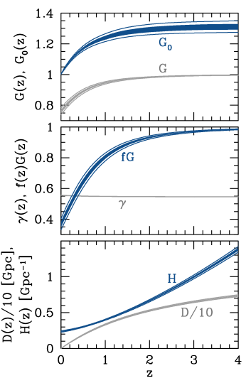
The strong predictions for flat $\Lambda$CDM arise largely due to CMB constraints: the two parameters $\Omega_{\rm m}$ and $H_{0}$ are tied together by the measurement of $\Omega_{\rm m}h^{2}$, and the remaining freedom in $H_{0}$ or the extragalactic distance scale is fixed by the measurement of the distance to $z_{*}$. However, given the present uncertainties in $\Omega_{\rm m}h^{2}$ and $D(z_{*})$, the addition of the other data (SN, BAO, and $H_{0}$) increases the precision of the predictions by almost a factor of 2 relative to WMAP constraints alone.

The flat $\Lambda$CDM model is therefore highly falsifiable in that future measurements may find that these quantities deviate substantially from the predictions. For example, an $H_{0}$ measurement with $\lesssim 2\%$ accuracy would match the precision of the predictions and hence provide a sharp test of flat $\Lambda$CDM. These predictions are only a factor of $2-3$ weaker than the Stage IV SN and CMB forecasts from MHH. Since flat $\Lambda$CDM is the current standard model of the cosmic expansion history and structure formation, falsifying it would represent the most important observational breakthrough since the discovery of cosmic acceleration and would require revision of basic assumptions about the nature of dark energy, spatial curvature, or the theory of gravity.

Figure 2: Predicted growth and expansion observables for non-flat (dark blue) and flat (light gray) $\Lambda$CDM, plotted relative to the reference cosmology (the best fit model for flat $\Lambda$CDM). Here and in subsequent figures, 68% CL regions are marked by shading, 95% CL regions are bounded by solid curves, and red curves outlined in white show the best fit model of the more general (dark blue) model class (in this case, non-flat $\Lambda$CDM).

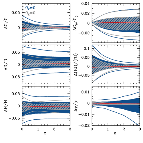
Generalizing the model to $\Lambda$CDM with curvature increases the range of predictions by less than a factor of 2. In Fig. 2, we plot the predictions for flat and non-flat $\Lambda$CDM relative to the ML flat $\Lambda$CDM model with $\Omega_{\rm m}=0.268$, $h=0.711$. Curvature opens up the ability to free the extragalactic distance scale from the constraints imposed by the CMB acoustic peak measurements. The tight constraints on SN, $H_{0}$, and BAO distances limit this freedom. Since the forecasts from MHH used only the current BAO measurement and a weaker $H_{0}$ constraint as priors, the relative impact of curvature here is substantially smaller. In particular, predictions of the growth function are nearly unchanged by curvature and still vary by less than $2\%$. Likewise, $fG$ is nearly unaffected by curvature. Although the growth index, $\gamma(z)$, is not as perfectly determined for non-flat $\Lambda$CDM, especially at high redshift, it is still predicted to better than 1% at $z\lesssim 3$, and both $D(z)$ and $H(z)$ are predicted to better than $3\%$. Any measurement that deviates by significantly more than these amounts would prove that the dark energy is not a cosmological constant.

III.2 Quintessence

Figure 3: Flat quintessence models without early dark energy (dark blue) vs. flat $\Lambda$CDM (light gray). Other aspects here and in later figures follow Fig. 2.

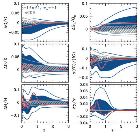
If $\Lambda$CDM is falsified, then in the context of dark energy we must consider models with $w(z)\neq-1$. Our next class of models are therefore flat quintessence models with $w(z)$ parametrized by 10 principal components at $z<1.7$, assuming no early dark energy (“$w_{\infty}=-1$”). The predictions for acceleration observables within this model class are compared with the flat $\Lambda$CDM predictions in Fig. 3.

Interestingly, the quintessence predictions are no longer centered on the flat $\Lambda$CDM ML model. From the $H(z)$ predictions which mainly reflect variation in evolution of the dark energy density, we see that on average the data favor a smaller low-redshift ($z\lesssim 0.5$) and larger intermediate-redshift ($0.5\lesssim z\lesssim 2$) dark energy density. Correspondingly, the best fit growth function $G(z)$ of $\Lambda$CDM is higher than that of $\sim 85\%$ of the quintessence models in the chain. Therefore a measurement of the growth relative to high redshift that is smaller than the $\Lambda$CDM prediction by more than a few percent not only rules out a cosmological constant but actually favors these quintessence models. The additional freedom in growth opens up predictions for $\gamma$ to include $2-3\%$ deviations at $z\lesssim 1$.

Figure 4: Upper panel: Comparison of distance constraints from SN data and best fit models, plotted relative to the best fit $H_{0}D(z)$ for flat $\Lambda$CDM (dotted line). Blue points with error bars show the Union SN data in redshift bins of width $\Delta\log z=0.05$. The best fit model for flat quintessence without early dark energy is plotted as a dashed curve, and the solid curve shows how the relative distances are affected by smoothing $w(z)$ for this model by a Gaussian of width $\sigma_{z}=0.1$. The full distribution of relative distance predictions for this quintessence model class is also shown with light gray shading (68% CL) and curves (95% CL). Lower panel: $w(z)$ for each of the models from the upper panel.

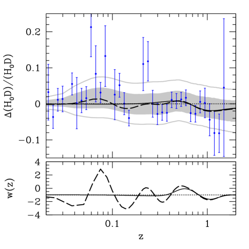
Many of the shifts in the predictions relative to flat $\Lambda$CDM are reflected in the evolution of $w(z)$ in the maximum likelihood model for flat quintessence without early dark energy. The ML model in this class marginally improves the fit to the current data sets relative to the $\Lambda$CDM ML model, largely due to variations in the SN data with redshift that are fit marginally better by dynamical dark energy than by a cosmological constant. Figure 4 compares ML models, quintessence predictions, and relative distance constraints from the Union SN data sets at $z\lesssim 1$. Freedom in $w(z)$ at these redshifts allows changes in the dark energy density to improve the fit to SN distances by $-2\Delta\ln\mathcal{L}\sim 4.5$. However, some of this improvement is due to the large oscillations in the equation of state at $z\sim 0.1$, which are allowed to violate the $-1\leq w\leq 1$ bound due to the conservative implementation of the quintessence prior on PC amplitudes described in Sec. II.3. Smoothing the ML $w(z)$ by a Gaussian with width $\sigma_{z}\sim 0.1$ or requiring $w(z)$ to satisfy stricter quintessence bounds reduces the improvement relative to $\Lambda$CDM to $-2\Delta\ln\mathcal{L}\sim 2$, but has little effect on the overall distributions of the predicted observables.

Although differences in the ML models cause quintessence to not be centered around $\Lambda$CDM, the allowed width of quintessence predictions around the maximum likelihood relative to $\Lambda$CDM follows the expectations of the Stage IV predictions from MHH except for being weaker by a factor of $2-3$. The PCs allow for oscillatory variations in $H(z)$, $f(z)G(z)$, and $\gamma(z)$ at $z<1$ that would not be readily observable with expansion history or growth measures due to limited resolution in redshift. On the other hand, $G(z)$, $G_{0}(z)$, and $D(z)$ are still predicted with $\sim 2-3\%$ precision, so the class of flat quintessence models without early dark energy remains highly falsifiable.

Figure 5: Flat quintessence models with (dark blue) and without (light gray) early dark energy.

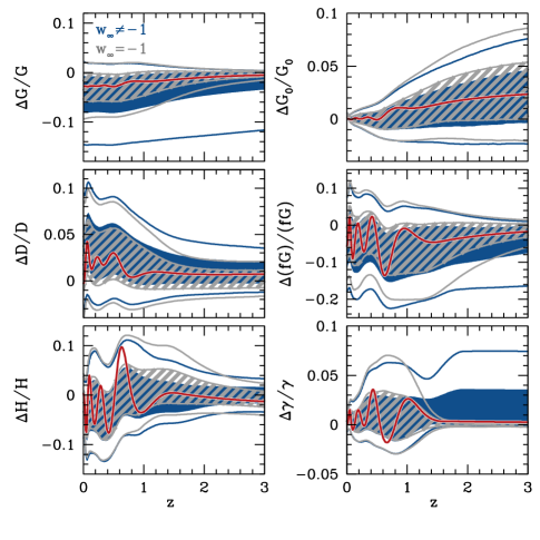
Adding early dark energy to flat quintessence (Fig. 5) has very little impact on the 68% CL predictions of most observables due to the restriction that $w\geq-1$ for a canonical scalar field. To satisfy CMB distance constraints, any increase in the expansion rate due to early dark energy must be compensated by a lower expansion rate at intermediate redshift relative to $z=0$, i.e. a dark energy density that decreases with increasing redshift requiring $w<-1$. While adding early dark energy does allow a larger suppression of growth at high redshift (which is also a possible sign of massive neutrinos given current upper limits), a measurement of a $\gtrsim 10-15\%$ decrement or $\gtrsim 2\%$ increment in the growth relative to high redshift would still suggest that a broader class of models is necessary. This freedom in growth leaves the amplitude relative to $z=0$ practically unchanged as the $G_{0}(z)$ predictions show. The only qualitative change with early dark energy is to open up the allowed range in $\gamma(z)$ so that the high redshift end has as much freedom as the low redshift end. All of these trends for early dark energy without curvature reflect those of the forecasts in MHH.

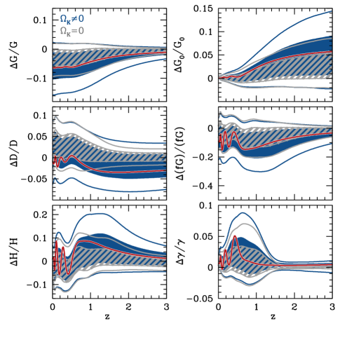
Including curvature in the quintessence class, but not early dark energy, opens up more freedom as shown in Fig. 6. Now $z>2$ deviations in $D(z)$ are allowed at the $\sim 5\%$ level relative to $\Lambda$CDM. Thus a BAO distance measurement at $z>2$ could falsify flat quintessence in favor of quintessence with curvature. As discussed in MHH, because of the $w\geq-1$ quintessence bound, this additional freedom skews to smaller distances and lower growth relative to high redshift.

Figure 6: Non-flat (dark blue) and flat (light gray) quintessence models without early dark energy.

Predictions from the most general quintessence class which includes both curvature and early dark energy, shown in Fig. 7, combine features of the previous quintessence classes in ways that are similar to the Stage IV predictions in MHH. The ML model in this class improves the fit to the combined data by $-2\Delta\ln\mathcal{L}\sim 4$, mostly due to changing the SN likelihood by $-2\Delta\ln\mathcal{L}\sim 5$; however, removing the large low-$z$ oscillations by smoothing $w(z)$ reduces the improvement in the SN fit to $-2\Delta\ln\mathcal{L}\sim 2-3$.

Figure 7: Non-flat quintessence models with (dark blue) and without (light gray) early dark energy.

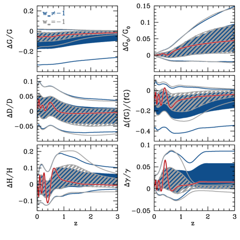
The predictions for $G_{0}(z)$, $D(z)$, and $H(z)$, which were affected little by early dark energy alone, are nearly the same as those for non-flat quintessence without early dark energy. The other observables show a mixture of the effects of curvature at low $z$ and early dark energy at high $z$. Large suppression ($\gtrsim 20\%$) of $G(z)$ (and similarly $fG$) relative to $\Lambda$CDM is allowed, but enhancement of the growth function over the $\Lambda$CDM best fit is still limited at the $\sim 2\%$ level. Note that this upper limit on $G(z)$ is robust to neutrino mass uncertainties. Likewise, low-redshift distances (including $z_{h}H_{0}^{-1}$) cannot be smaller than in $\Lambda$CDM by substantially more than $\sim 2\%$. As in Fig. 5, the high redshift predictions for $\gamma(z)$ in Fig. 7 weaken substantially but only in the positive direction. Indeed, all of the observables display similar asymmetric weakening of the predictions with the addition of curvature and early dark energy, which can be understood in terms of the $w\geq-1$ quintessence bound.

The existence of an upper or lower bound on each observable that is robust to freedom in curvature and early dark energy provides the possibility of falsifying the entire quintessence model class. In fact, in this most general class, the statistical predictions from current SN and CMB bounds are already comparable to those that can be achieved by a Stage IV version of these probes, which can be understood from the fact that the forecasts from MHH used current BAO and $H_{0}$ measurements.

The comparable predictions in large part reflect the fact that curvature is already well constrained through the BAO and $H_{0}$ measurements. The constraint in this most general class of quintessence models is $-0.006<\Omega_{K}<0.033$ (95% CL), a factor of $\sim 2$ weaker than for non-flat $\Lambda$CDM and skewed toward open models due to the quintessence prior on $w(z)$.

Finally, as an example of the use of the asymmetric quintessence predictions, we consider the application of these results to observables which measure some combination of $\sigma_{8}$ and $\Omega_{\rm m}$. To compute predictions for $\sigma_{8}$ given our predictions for the raw acceleration observables, we use the fitting formula Hu_Jain

$$\sigma_{8} = \frac{G(z=0)}{0.76}\left[\frac{A_{s}(k=0.05~{}{\rm Mpc}^{-1})}{3.12\times 10^{-9}}\right]^{1/2}\left(\frac{\Omega_{\rm b}h^{2}}{0.024}\right)^{-1/3}$$ (11)

$$\times\left(\frac{\Omega_{\rm m}h^{2}}{0.14}\right)^{0.563}\left(\frac{h}{0.72}\right)^{0.693}(3.123h)^{(n_{s}-1)/2}$$

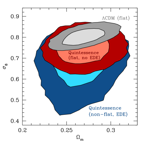
for each model sampled in the MCMC likelihood analysis. Note that on top of allowed variations in $G(z=0)$, $\sigma_{8}$ predictions include uncertainties in the reionization optical depth $\tau$ through its covariance with $A_{s}$. While this analysis assumes instantaneous reionization, the uncertainty introduced by more general ionization histories is small MorHu08 . We have checked that the $\sigma_{8}$ distributions obtained using Eq. (11) closely match those from the more accurate computation of $\sigma_{8}$ using CAMB. The joint predictions for $\sigma_{8}$ and $\Omega_{\rm m}$ from the current SN, CMB, BAO, and $H_{0}$ constraints are shown in Fig. 8 for flat $\Lambda$CDM and two quintessence model classes.

In particular, in the context of flat $\Lambda$CDM the current SN, CMB, BAO, and $H_{0}$ data predict the combination best measured by the local abundance of massive galaxy clusters to be $0.394<\sigma_{8}\Omega_{\rm m}^{0.5}<0.441$ (68% CL). Flat quintessence without early dark energy weakens the lower end somewhat but leaves the upper limit nearly unchanged: $0.358<\sigma_{8}\Omega_{\rm m}^{0.5}<0.419$. Quintessence with both early dark energy and curvature yields $0.306<\sigma_{8}\Omega_{\rm m}^{0.5}<0.396$. Therefore a measurement of a local cluster abundance in significant excess of the flat $\Lambda$CDM predictions rules out the whole quintessence class, whereas a measurement that is substantially lower would remain consistent with quintessence but would rule out a cosmological constant (see also Kunz_sigma8 ). A measurement below the flat $\Lambda$CDM prediction by $\lesssim 10\%$ could also indicate large neutrino masses, but an excess cluster abundance could not be alternately explained by massive neutrinos. Current cluster surveys, with $\sim 5\%$ measurements of similar combinations of $\sigma_{8}$ and $\Omega_{\rm m}$ Vikhlinin ; Rozo ; Mantz , are beginning to reach the precision necessary to test these predictions. In fact, the lack of an observed excess already places strong constraints on modified gravity explanations of cosmic acceleration Schmidt:2009am .

Figure 8: Predictions for $\sigma_{8}$ and $\Omega_{\rm m}$ for flat $\Lambda$CDM (gray contours, top), flat quintessence without early dark energy (red contours, middle), and non-flat quintessence with early dark energy (blue contours, bottom), showing 68% CL (light) and 95% CL (dark) regions.

III.3 Smooth $w_{0}-w_{a}$ Dark Energy

As a final case we consider the class of models defined by an equation of state $w(z)=w_{0}+(1-a)w_{a}$ Chevallier_Polarski ; Linder_wa under the assumption that dark energy is smooth relative to matter. Unlike our previous cases, this class does not define a physical candidate for dark energy such as the cosmological constant or a scalar field but rather represents a simple but illustrative phenomenological parametrization. Note that early dark energy is included in this parametrization since $\lim_{z\to\infty}w(z)=w_{0}+w_{a}$.

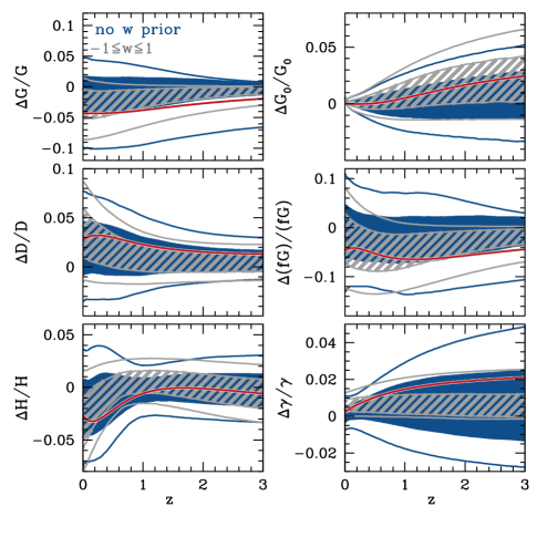
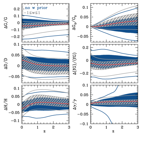
The predictions for the $w_{0}-w_{a}$ model class serve two purposes. First, the comparison of predictions for smooth, monotonic $w_{0}-w_{a}$ models with those for PC quintessence models test the dependence of the predictions on rapid transitions and non-monotonic evolution of the equation of state. The second use of the $w_{0}-w_{a}$ predictions is to illustrate how predictions are affected by the $-1\leq w(z)\leq 1$ quintessence bound. Unlike the model classes where $w(z)$ is parametrized by principal components, it is simple to impose a strict quintessence prior on $w_{0}-w_{a}$ models by requiring $-1\leq w_{0}\leq 1$ and $-1\leq w_{0}+w_{a}\leq 1$. We compare predictions using this prior with the more general case, where the priors are weak enough that constraints on $w_{0}$ and $w_{a}$ are determined solely by the data (“no $w$ prior”).

A fair comparison can be made between the predictions for flat and non-flat $w_{0}-w_{a}$ models with the $-1\leq w\leq 1$ prior (light gray contours in Figs. 9 and 10) and PC quintessence models with early dark energy (dark blue contours in Figs. 5 and 7). In particular, observables relatively insensitive to both the amount of early dark energy and large changes in the PC equation of state at low redshift, such as $G_{0}(z)$ and $D(z)$, are generally in good agreement. The expansion rate and growth rate are more sensitive to sudden changes in $w(z)$ than the distances and the integrated growth function. Therefore, the impact of large, low-$z$ oscillations in the PCs is greatest for $H(z)$, $f(z)G(z)$, and $\gamma(z)$ at $z\lesssim 1$, increasing the width of those predictions relative to the corresponding predictions for the smooth $w_{0}-w_{a}$ models. The PC quintessence models also have more freedom in early dark energy than $w_{0}-w_{a}$ models since $w_{\infty}$, unlike $w_{0}+w_{a}$, is completely free from the low-redshift SN, BAO, and $H_{0}$ constraints. As a result, $w_{0}-w_{a}$ predictions for $G(z)$ and the high-redshift values of $\gamma(z)$ and $f(z)G(z)$ are stronger than, but still qualitatively similar to, those for PC quintessence with early dark energy.

Like the PC quintessence predictions, the predictions for $w_{0}-w_{a}$ models bounded by $-1\leq w\leq 1$ are shifted relative to flat $\Lambda$CDM due to marginal improvements in the fit to SN data ($-2\Delta\ln\mathcal{L}\sim 0.5$ for the ML model) enabled by an evolving equation of state. This is a somewhat smaller change in the likelihood than for PC quintessence models, but the magnitude of the ML model shift in the observables is similar for $w_{0}-w_{a}$ and PC quintessence, at least for those observables that depend little on early dark energy.

Comparing the two sets of predictions in Figs. 9 and 10 (no $w$ prior vs. the $-1\leq w\leq 1$ prior) shows the effect on the $w_{0}-w_{a}$ predictions of allowing freedom in $w(z)$ beyond that allowed by the quintessence bounds. As discussed in MHH, eliminating these bounds makes the range in predictions for observables such as growth more symmetric around the best fit for flat $\Lambda$CDM since $w(z)$ is allowed to cross below $w=-1$. In particular, growth in excess of flat $\Lambda$CDM is now allowed. Based on the analysis of MHH, we expect the amount of the remaining skewness in the predictions around flat $\Lambda$CDM to be affected by the available volume of parameter space as determined by how priors on dark energy parameters weight models with $w<-1$ relative to those with $w>-1$.

Removing the quintessence bounds also allows models with greater amounts of early dark energy, and (for non-flat $w_{0}-w_{a}$) more closed models, to fit the data. A notable consequence for models with nonzero curvature is that the predictions for $\gamma(z)$ at 95% CL diverge at $z>1$. This is the same effect noted in MHH for $\gamma(z)$ forecasts in the non-flat smooth dark energy model class. The divergence in the tails of the high-redshift $\gamma(z)$ distribution is caused by the appearance of a singularity in $\gamma(z)$ for closed models where $\Omega_{\rm K}$ is sufficiently negative so that $\Omega_{\rm m}(z)$ crosses unity at some redshift; when $\Omega_{\rm m}(z)=1$, $\gamma(z)$ is no longer well defined by Eq. (6). Such caveats must be kept in mind when using $\gamma$ as a test of not only quintessence but of all smooth dark energy models.

Figure 9: Flat $w_{0}-w_{a}$ without priors on $w(z)$ (dark blue) and with quintessence priors ($-1\leq w_{0}\leq 1$, $-1\leq w_{0}+w_{a}\leq 1$; light gray).

Figure 10: Non-flat $w_{0}-w_{a}$ without priors on $w(z)$ (dark blue) and with quintessence priors ($-1\leq w_{0}\leq 1$, $-1\leq w_{0}+w_{a}\leq 1$; light gray).

IV Discussion

Any given class of dark energy models makes concrete predictions for the relationship between the expansion history, geometry, and growth of structure as a function of redshift. Therefore, current distance-based measurements, though limited in redshift, make predictions for other dark energy observables that can be used to test and potentially rule out whole classes of dark energy models.

In this paper we present the allowed ranges for the expansion rate $H(z)$, distances $D(z)$, the linear growth rate $G(z)$, and several auxiliary growth observables from the current combination of cosmological measurements of supernovae, the cosmic microwave background, baryon acoustic oscillations, and the Hubble constant. In particular, growth at any redshift or a Hubble constant in significant excess of $2\%$ ($68\%$ CL range) of the current best fit $\Lambda$CDM model would falsify both a cosmological constant and more general quintessence models with or without curvature and early dark energy. On the other hand, comparable measurements of a decrement in these quantities would rule out a cosmological constant but would be fully consistent with quintessence. Alternately, a substantial reduction in growth relative to the expectation for $\Lambda$CDM could indicate neutrinos with large masses ($\sum m_{\nu}>0.05$ eV).

Remarkably, predictions for the main acceleration observables, $H(z)$, $D(z)$, and $G(z)$, are only weaker than Stage IV SN and CMB predictions (MHH) by a factor of $\sim 2-3$. However, this improvement applies across a wide range of redshifts, indicating that multiple phenomenological parameters may each be improved by this factor. For example, parameter-based figures of merit effectively involve products of individual parameters (e.g. area in the $w_{0}-w_{a}$ plane Huterer_Turner ; DETF or volume of the principal component parameter error ellipsoid Albrecht_Bernstein ; FoMSWG ), and in such figures of merit the total improvement with future data can be significant. If novel dark energy physics affects small pockets of these high-dimensional parameter spaces — that is, if only specific dark energy parameter combinations are sensitive to new physics — then these multiparameter figures of merit will justly indicate a much more significant improvement with future cosmological data.

In this work we have considered only known and quantifiable sources of error in the current data. Recent analyses of supernova data (e.g. Constitution ; SDSS_SN ; Kelly09 ) indicate that unknown systematic errors remain and can significantly affect cosmological constraints. Furthermore, the systematic error estimates used here for the SN data were optimized for models with a cosmological constant and therefore may be underestimated for dynamical dark energy SCP_Union . We intend to explore the implications of SN systematics for dark energy predictions in future work. Our predictive methodology can alternately be viewed as a means of ferreting out unknown systematics by looking for inconsistencies between the predictions from one set of observations and data from another.

Over the course of this study, new data have become available that could improve the predictions for acceleration observables or begin to test predictions within the various classes. In particular, BAO measurements from SDSS DR7 and 2dFGRS provide a 2.7% constraint on $D_{V}(z=0.275)$ and a 3.7% constraint on $D_{V}(z=0.35)/D_{V}(z=0.2)$ Percival09 . We have estimated the impact of these new measurements on our predictions by using the updated BAO likelihood to modify the weighting of MCMC samples for each model class. For all quintessence model classes, the effect of updating the BAO data is negligible for most observables except for $D(z\lesssim 1)$ and (to a lesser extent) $H(z\lesssim 0.5)$, reflecting the improved BAO constraint on low-redshift $D$ and $H$.

The impact of the newer BAO measurements on $\Lambda$CDM models is greater than for quintessence since the reduced freedom in dark energy evolution ties low-redshift measurements to high-redshift predictions. The updated BAO constraints exclude models on one side of the predicted observable distributions in Fig. 2, reducing their width by $10-30\%$ and shifting the distributions by an equal amount. However, these changes appear to be mainly due to a slight tension between the new BAO constraints and the other data sets used for $\Lambda$CDM predictions. Note that the BAO constraints of Ref. Percival09 are still less precise than the flat $\Lambda$CDM predictions in Fig. 2 and comparable to the non-flat $\Lambda$CDM predictions, so they do not yet represent a significant additional test of the cosmological constant.

Falsifiable predictions from current data reveal many opportunities for sharp observational tests of paradigms for cosmic acceleration by requiring consistency within a given theoretical framework between observables that depend on the expansion history, geometry, and growth of structure in the universe. These predictions can be used to inform future surveys as to the optimal choice of observables, redshifts, and required measurement accuracies for testing whole classes of dark energy models. Falsification of even the simplest model, flat $\Lambda$CDM, would have revolutionary consequences for cosmology and fundamental physics.

Acknowledgments: We thank David Weinberg for useful conversations about this work. MM and WH were supported by the KICP under NSF contract PHY-0114422. MM was additionally supported by the NSF GRFP and CCAPP at Ohio State; WH by DOE contract DE-FG02-90ER-40560 and the Packard Foundation; DH by the DOE OJI grant under contract DE-FG02-95ER40899, NSF under contract AST-0807564, and NASA under contract NNX09AC89G.

References

- (1) D. N. Spergel et al., Astrophys. J. Suppl. 148, 175 (2003), [arXiv:astro-ph/0302209].
- (2) W. Hu, ASP Conf. Ser. 339, 215 (2005), [arXiv:astro-ph/0407158].
- (3) M. J. Mortonson, W. Hu and D. Huterer, Phys. Rev. D79, 023004 (2009), [arXiv:0810.1744], (MHH).
- (4) A. Albrecht et al., arXiv:astro-ph/0609591.
- (5) D. Huterer and A. Cooray, Phys. Rev. D71, 023506 (2005), [arXiv:astro-ph/0404062].
- (6) Y. Wang and M. Tegmark, Phys. Rev. D71, 103513 (2005), [arXiv:astro-ph/0501351].
- (7) A. G. Riess et al., Astrophys. J. 659, 98 (2007), [arXiv:astro-ph/0611572].
- (8) C. Zunckel and R. Trotta, Mon. Not. Roy. Astron. Soc. 380, 865 (2007), [arXiv:astro-ph/0702695].
- (9) S. Sullivan, A. Cooray and D. E. Holz, JCAP 0709, 004 (2007), [arXiv:0706.3730].
- (10) G.-B. Zhao, D. Huterer and X. Zhang, Phys. Rev. D77, 121302 (2008), [arXiv:0712.2277].
- (11) G.-B. Zhao and X. Zhang, arXiv:0908.1568.
- (12) P. Serra et al., arXiv:0908.3186.
- (13) J. Kujat, A. M. Linn, R. J. Scherrer and D. H. Weinberg, Astrophys. J. 572, 1 (2002), [arXiv:astro-ph/0112221].
- (14) S. Chongchitnan and G. Efstathiou, Phys. Rev. D76, 043508 (2007), [arXiv:0705.1955].
- (15) M. Sahlen, A. R. Liddle and D. Parkinson, Phys. Rev. D72, 083511 (2005), [arXiv:astro-ph/0506696].
- (16) D. Huterer and H. V. Peiris, Phys. Rev. D75, 083503 (2007), [arXiv:astro-ph/0610427].
- (17) H. Zhan, L. Knox and J. A. Tyson, Astrophys. J. 690, 923 (2009), [arXiv:0806.0937].
- (18) U. Dore and D. Orestano, Reports on Progress in Physics 71, 106201 (2008), [arXiv:0811.1194].
- (19) B. A. Reid et al., arXiv:0907.1659.
- (20) W. J. Percival and M. White, Mon. Not. R. Astron. Soc. 393, 297 (2009), [arXiv:0808.0003].
- (21) L. Wang and P. J. Steinhardt, Astrophys. J. 508, 483 (1998), [arXiv:astro-ph/9804015].
- (22) E. V. Linder, Phys. Rev. D72, 043529 (2005), [arXiv:astro-ph/0507263].
- (23) M. Kowalski et al., Astrophys. J. 686, 749 (2008), [arXiv:0804.4142].
- (24) http://supernova.lbl.gov/Union/.
- (25) E. Komatsu et al., Astrophys. J. Suppl. 180, 330 (2009), [arXiv:0803.0547].
- (26) M. R. Nolta et al., Astrophys. J. Suppl. 180, 296 (2009), [arXiv:0803.0593].
- (27) J. Dunkley et al., Astrophys. J. Suppl. 180, 306 (2009), [arXiv:0803.0586].
- (28) http://lambda.gsfc.nasa.gov/.
- (29) A. Lewis, A. Challinor and A. Lasenby, Astrophys. J. 538, 473 (2000), [arXiv:astro-ph/9911177].
- (30) http://camb.info/.
- (31) W. Fang, W. Hu and A. Lewis, Phys. Rev. D78, 087303 (2008), [arXiv:0808.3125].
- (32) http://camb.info/ppf/.
- (33) D. J. Eisenstein et al., Astrophys. J. 633, 560 (2005), [arXiv:astro-ph/0501171].
- (34) W. J. Percival et al., Mon. Not. R. Astron. Soc. (2009), [arXiv:0907.1660].
- (35) A. G. Riess et al., Astrophys. J. 699, 539 (2009), [arXiv:0905.0695].
- (36) M. Mortonson, W. Hu and D. Huterer, Phys. Rev. D80, 067301 (2009), [arXiv:0908.1408].
- (37) D. Huterer and G. Starkman, Phys. Rev. Lett. 90, 031301 (2003), [arXiv:astro-ph/0207517].
- (38) W. Hu, Phys. Rev. D66, 083515 (2002), [arXiv:astro-ph/0208093].
- (39) G. Aldering et al., arXiv:astro-ph/0405232.
- (40) J. Samsing and E. V. Linder, arXiv:0908.2637.
- (41) N. Christensen, R. Meyer, L. Knox and B. Luey, Class. Quant. Grav. 18, 2677 (2001), [arXiv:astro-ph/0103134].
- (42) A. Kosowsky, M. Milosavljevic and R. Jimenez, Phys. Rev. D66, 063007 (2002), [arXiv:astro-ph/0206014].
- (43) J. Dunkley, M. Bucher, P. G. Ferreira, K. Moodley and C. Skordis, Mon. Not. R. Astron. Soc. 356, 925 (2005), [arXiv:astro-ph/0405462].
- (44) A. Lewis and S. Bridle, Phys. Rev. D66, 103511 (2002), [arXiv:astro-ph/0205436].
- (45) http://cosmologist.info/cosmomc/.
- (46) A. Gelman and D. Rubin, Statistical Science 7, 452 (1992).
- (47) W. Hu and B. Jain, Phys. Rev. D70, 043009 (2004), [arXiv:astro-ph/0312395].
- (48) M. J. Mortonson and W. Hu, Astrophys. J. 672, 737 (2008), [arXiv:0705.1132].
- (49) M. Kunz, P. S. Corasaniti, D. Parkinson and E. J. Copeland, Phys. Rev. D70, 041301 (2004), [arXiv:astro-ph/0307346].
- (50) A. Vikhlinin et al., Astrophys. J. 692, 1060 (2009), [arXiv:0812.2720].
- (51) E. Rozo et al., arXiv:0902.3702.
- (52) A. Mantz, S. W. Allen, D. Rapetti and H. Ebeling, arXiv:0909.3098.
- (53) F. Schmidt, A. Vikhlinin and W. Hu, Phys. Rev. D80, 083505 (2009), [arXiv:0908.2457].
- (54) M. Chevallier and D. Polarski, Int. J. Mod. Phys. D10, 213 (2001), [arXiv:gr-qc/0009008].
- (55) E. V. Linder, Phys. Rev. Lett. 90, 091301 (2003), [arXiv:astro-ph/0208512].
- (56) D. Huterer and M. S. Turner, Phys. Rev. D64, 123527 (2001), [arXiv:astro-ph/0012510].
- (57) A. J. Albrecht and G. Bernstein, Phys. Rev. D75, 103003 (2007), [arXiv:astro-ph/0608269].
- (58) A. J. Albrecht et al., arXiv:0901.0721.
- (59) R. Kessler et al., Astrophys. J. Suppl. 185, 32 (2009), [arXiv:0908.4274].
- (60) P. L. Kelly, M. Hicken, D. L. Burke, K. S. Mandel and R. P. Kirshner, arXiv:0912.0929.
- (61) M. Hicken et al., Astrophys. J. 700, 1097 (2009), [arXiv:0901.4804].