The effects of LIGO detector noise on a 15-dimensional Markov-chain Monte-Carlo analysis of gravitational-wave signals

Abstract

Gravitational-wave signals from inspirals of binary compact objects (black holes and neutron stars) are primary targets of the ongoing searches by ground-based gravitational-wave (GW) interferometers (LIGO, Virgo, and GEO-600). We present parameter-estimation results from our Markov-chain Monte-Carlo code SPINspiral on signals from binaries with precessing spins. Two data sets are created by injecting simulated GW signals into either synthetic Gaussian noise or into LIGO detector data. We compute the 15-dimensional probability-density functions (PDFs) for both data sets, as well as for a data set containing LIGO data with a known, loud artefact (“glitch”). We show that the analysis of the signal in detector noise yields accuracies similar to those obtained using simulated Gaussian noise. We also find that while the Markov chains from the glitch do not converge, the PDFs would look consistent with a GW signal present in the data. While our parameter-estimation results are encouraging, further investigations into how to differentiate an actual GW signal from noise are necessary.

1 Introduction

Among the sources of gravitational waves (GWs), inspiralling binary systems of compact objects, neutron stars (NSs) and/or black holes (BHs) in the mass range $\sim 1\,M_{\odot}-100\,M_{\odot}$ stand out as likely to be detected and relatively easy to model. For ground-based laser interferometers currently in operation [2002gr.qc.....4090C], LIGO [2009NJPh...11g3032A], Virgo [2008CQGra..25r4001A] and GEO-600 [2004CQGra..21S.417W], the current detection-rate estimates for BH-NS binaries range from $2\times 10^{-4}$ to $0.2$ yr^-1 for first-generation instruments 2008ApJ…672..479O,2010arXiv1003.2480Le.g.. Although the estimates are quite uncertain, detection rates are expected to increase with the upgrade to Enhanced LIGO/Virgo, up to $\sim 40$ yr^-1 with Advanced LIGO/Virgo.

The detection of a gravitational-wave event is challenging and will be a rewarding achievement by itself. After such a detection, measurement of source properties holds major promise for improving our astrophysical understanding and requires reliable methods for parameter estimation. This is a complicated problem, because of the large number of parameters ($15$ for spinning compact objects in a quasi-circular orbit) and the degeneracies between them [2009CQGra..26k4007R], the significant amount of structure in the parameter space, and the particularities of the detector noise.

In this paper we use an example to illustrate the capabilities of our Markov-chain Monte-Carlo (MCMC) algorithm SPINspiral [2008CQGra..25r4011V] for parameter estimation of binary inspirals with two spinning components, using ground-based GW interferometers. In these proceedings we focus on the effects of using LIGO detector data versus synthetic Gaussian noise. Earlier studies 1994PhRvD..49.1723J,1994PhRvD..49.2658C,1995PhRvD..52..848P,2007CQGra..24.1089Ve.g. computed the potential accuracy of parameter estimation (e.g. by using the Fisher matrix), but without performing a parameter estimation in practice. Also, 2006CQGra..23.4895R 2006CQGra..23.4895R,2007PhRvD..75f2004R, 2009arXiv0911.3820V 2008PhRvD..78b2001V,2008CQGra..25r4010V,2009arXiv0911.3820V explored parameter estimation for binaries without spins, described by nine parameters.

We present the gravitational-wave template used for this study in section  2, and the Bayesian framework we employ here in section  3. In section 4.1 we describe the three data sets that we analyse in this study; a simulated GW signal injected into synthetic Gaussian noise, a GW signal injected into LIGO detector data and a raw LIGO data set containing a known artefact of terrestrial origin (“glitch”). We describe the details of the MCMC simulations in section 4.2. The analyses of the first two data sets are compared in section 4.3, and we present our results on the glitch in section  4.4.

2 Gravitational-wave signal and observables

We analyse the signal produced during the inspiral phase of two compact objects of masses $M_{1,2}$ in quasi-circular orbit. We focus on a black-hole binary system with $M_{1}=10\,M_{\odot}$ and $M_{2}=1.4\,M_{\odot}$, where unlike in some of our previous studies 2008ApJ…688L..61Ve.g., we do not ignore the second spin to explore the single spin approximation. During the orbital inspiral, the general-relativistic spin-orbit and spin-spin coupling (dragging of inertial frames) cause the binary’s orbital plane to precess and introduce amplitude and phase modulations of the observed gravitational-wave signal [1994PhRvD..49.6274A].

A circular binary inspiral with both compact objects spinning is described by a 15-dimensional parameter vector $\vec{\lambda}\in\Lambda$. Our choice of independent parameters with respect to a fixed geocentric coordinate system is:

$$\vec{\lambda}= \{{\cal M},\eta,\log{d_{\mathrm{L}}},t_{\mathrm{c}},\phi_{\mathrm{c}},\alpha,\cos\delta,\sin{\iota},\psi,$$ (1)

$$a_{\mathrm{spin1}},\cos\theta_{\mathrm{spin1}},\phi_{\mathrm{spin1}},a_{\mathrm{spin2}},\cos\theta_{\mathrm{spin2}},\phi_{\mathrm{spin2}}\},$$

where ${\cal M}=\frac{(M_{1}M_{2})^{3/5}}{(M_{1}+M_{2})^{1/5}}$ and $\eta=\frac{M_{1}M_{2}}{(M_{1}+M_{2})^{2}}$ are the chirp mass and symmetric mass ratio, respectively; $d_{\mathrm{L}}$ is the luminosity distance to the source; $\phi_{\mathrm{c}}$ is an integration constant that specifies the GW phase at the time of coalescence $t_{\mathrm{c}}$, defined with respect to the centre of the Earth; $\alpha$ (right ascension) and $\delta$ (declination) identify the source position in the sky; $\iota$ defines the inclination of the binary with respect to the line of sight; and $\psi$ is the polarisation angle of the waveform. The spins are specified by $0\leq a_{\mathrm{spin_{1,2}}}\equiv S_{1,2}/M_{1,2}^{2}\leq 1$ as the dimensionless spin magnitude, and the angles $\theta_{\mathrm{spin1,2}}$,$\phi_{\mathrm{spin1,2}}$ for their orientations.

Given a network comprising $n_{\mathrm{det}}$ detectors, the data collected at the $a-$th instrument ($a=1,\dots,n_{\mathrm{det}}$) is given by $x_{a}(t)=n_{a}(t)+h_{a}(t;\vec{\lambda})$, where $h_{a}(t;\vec{\lambda})=F_{a,+}(t,\alpha,\delta,\psi)\,h_{a,+}(t;\vec{\lambda})+F_{a,\times}(t,\alpha,\delta,\psi)\,h_{a,\times}(t;\vec{\lambda})$ is the GW strain at the detector 1994PhRvD..49.6274Asee Eqs. 2–5 in and $n_{a}(t)$ is the detector noise. The astrophysical signal is given by the linear combination of the two independent polarisations $h_{a,+}(t;\vec{\lambda})$ and $h_{a,\times}(t;\vec{\lambda})$ weighted by the antenna beam patterns $F_{a,+}(t,\alpha,\delta,\psi)$ and $F_{a,\times}(t,\alpha,\delta,\psi)$.

The waveform we use includes terms up to ${3.5}$-post-Newtonian (pN) order in phase and uses Newtonian amplitudes, with spin effects up to ${2.5}$-pN in phase. We generate the waveform templates using the routine LALGenerateInspiral() with the approximant SpinTaylor from the injection package in the LSC Algorithm Library (LAL) [LAL], which closely follows the first section of 2003PhRvD..67j4025B 2003PhRvD..67j4025B.

3 Parameter estimation: Methods

In our Bayesian analysis we use MCMC methods to determine the multi-dimensional posterior probability-density function (PDF) of the unknown parameter vector $\vec{\lambda}$ in equation 1, given the data sets $x_{a}$ collected by a network of $n_{\mathrm{det}}$ detectors, a model $M$ of the waveform and the prior $p(\vec{\lambda})$ on the parameters. Our priors are uniform in the parameters of Eq. 1 (see 2008CQGra..25r4011V for details). One can compute the probability density via Bayes’ theorem

$$p(\vec{\lambda}|x_{a},M)=\frac{p(\vec{\lambda}|M)\,p(x_{a}|\vec{\lambda},M)}{p(x_{a}|M)}\,,$$ (2)

where

$$\mathcal{L}\equiv p(x_{a}|\vec{\lambda},M)\propto\exp\left(<x_{a}|h_{a}(\vec{\lambda})>-\frac{1}{2}<h_{a}(\vec{\lambda})|h_{a}(\vec{\lambda})>\right)$$ (3)

is the likelihood function, which measures how well the data fits the model $M$ for the parameter vector $\vec{\lambda}$. The term $p(x_{a}|M)$ is the marginal likelihood or evidence. In the previous equation

$$<x|y>=4Re\left(\int_{f_{\rm low}}^{f_{\rm high}}\frac{\tilde{x}(f)\tilde{y}^{*}(f)}{S_{a}(f)}\,\mathrm{d}f\right)$$ (4)

is the overlap of signals $x$ and $y$, $\tilde{x}(f)$ is the Fourier transform of $x(t)$, and $S_{a}(f)$ is the noise power-spectral density in detector $a$. The likelihood computed for the injection parameters $\mathcal{L}_{\mathrm{inj}}=p(x_{a}|\vec{\lambda}_{\mathrm{inj}},M)$ is then a random variable that depends on the particular noise realisation $n_{a}$ in the data $x_{a}=h(\vec{\lambda}_{\mathrm{inj}})+n_{a}$. The injection parameters are the parameters of the waveform template added to the noise. We define the signal-to-noise ratio (SNR) of the injection to be:

$$\mathrm{SNR}=\frac{<x|h(\vec{\lambda}_{\rm inj})>}{\sqrt{<h(\vec{\lambda}_{\rm inj})|h(\vec{\lambda}_{\rm inj})>}}.$$ (5)

From here on, we use the expected value of the SNR, which is equal to the square root of twice the expectation value of $\log{\cal L_{\mathrm{inj}}}$:

$$\mathrm{SNR}=\sqrt{<h(\vec{\lambda}_{\mathrm{inj}})|h(\vec{\lambda}_{\mathrm{inj}})>}.$$ (6)

To combine observations from a network of detectors with uncorrelated noise realisations (this is the case in this paper as we use two non-co-located detectors) we have the likelihood $p(\vec{x}|\vec{\lambda},M)=\prod_{a=1}^{n_{\mathrm{det}}}\,p(x_{a}|\vec{\lambda},M)\,$, for $\vec{x}\equiv\{x_{a}:a=1,\dots,n_{\mathrm{det}}\}$ and

$$p(\vec{\lambda}|\vec{x},M)=\frac{p(\vec{\lambda}|M)\,p(\vec{x}|\vec{\lambda},M)}{p(\vec{x}|M)}.$$ (7)

The numerical computation of the PDF involves the evaluation of a large multi-modal, multi-dimensional integral. Markov-chain Monte-Carlo (MCMC) methods [and references therein]gilks_etal_1996,gelman_etal_1997e.g. have proved to be especially effective in tackling this numerical problem. We developed an adaptive figueiredo_jain_2002,atchade_rosenthal_2005see MCMC algorithm to explore the parameter space $\Lambda$ efficiently while requiring the least amount of tuning for the specific signal analysed; the code is an extension of the one developed by some of the authors to explore MCMC methods for binaries without spin [2006CQGra..23.4895R, 2007PhRvD..75f2004R]. We implemented parallel tempering [1996JPSJ...65.1604H, 1997CPL...281..140H, 2007PhD..Auck] to improve the sampling. It consists of running several MCMC chains in parallel, each with a different “temperature”, which can swap parameters under certain conditions. Only the $T=1$ chain is currently used for post-processing.

In Eq. 7 we applied Bayes’ theorem to obtain the probability of a specific parameter vector value ($\vec{\lambda}$) given the observed data $\vec{x}$ and the model $M$. The theorem can also be applied to compute the probability of a specific model $M_{i}$ given the observed data:

$$p(M_{i}|\vec{x})=\frac{p(M_{i})\,p(\vec{x}|M_{i})}{p(\vec{x})}.$$ (8)

We compare the two models $M_{i}$ and $M_{j}$ by computing the odds ratio:

$$O_{i,j}=\frac{p(M_{i}|\vec{x})}{p(M_{j}|\vec{x})}=\frac{p(M_{i})\,p(\vec{x}|M_{i})}{p(M_{j})\,p(\vec{x}|M_{j})}=\frac{p(M_{i})}{p(M_{j})}B_{i,j},$$ (9)

where

$$B_{i,j}=\frac{p(\vec{x}|M_{i})}{p(\vec{x}|M_{j})}$$ (10)

is the Bayes factor of the two models, and we recognise the evidence $p(\vec{x}|M_{i})$ from Eq. 7. The evidence must be marginalised over the parameters of the model in order to compute the Bayes factor:

$$p(\vec{x}|M_{i})=\int_{\Lambda}p(\vec{\lambda}|M_{i})\,p(\vec{x}|\vec{\lambda},M_{i})\,\mathrm{d}\vec{\lambda}.$$ (11)

There are existing algorithms dedicated to the computation of this integral, and of the Bayes factor. For instance, nested sampling [MR2282208] has been shown to be very efficient in the case of non-spinning gravitational-wave sources [2009arXiv0911.3820V], and can in addition be used to produce PDFs of the parameters. As a by-product of the exploration of the parameter space with MCMC, it is possible to compute the evidences of the models used. We have implemented the harmonic-mean method [1994JSTOR..N], in which the evidence is approximated by:

$$p(\vec{x}|M_{i})\,\approx\,\sum_{k=1}^{N}p(\vec{\lambda}_{k}|M_{i})\,p(\vec{x}|\vec{\lambda}_{k},M_{i})\,V_{\vec{\lambda}_{k}},$$ (12)

where $\{\vec{\lambda}_{k}:k=1,\dots,N\}$ is the set of $N$ points sampled by the MCMC, and $V_{\vec{\lambda}_{k}}$ is the volume of parameter space associated with the point $\vec{\lambda}_{k}$. Since the MCMC algorithm samples according to the posterior (and, up to a proportionality constant, converges towards posterior PDF), the density of points in the chain at a certain location $\vec{\lambda}_{k}$ in the parameter space $\Lambda$ will become proportional to the posterior for large $N$. It follows that

$$\lim_{N\to\infty}\,V_{\vec{\lambda}_{k}}=\frac{\alpha_{i}}{p(\vec{\lambda}_{k}|M_{i})\,p(\vec{x}|\vec{\lambda}_{k},M_{i})},$$ (13)

with $\alpha_{i}$ a proportionality constant. We then have $p(\vec{x}|M_{i})\,\approx\,\sum_{k=1}^{N}\alpha_{i}=N\,\alpha_{i}$, and obtain the estimate for $\alpha_{i}$ by considering the whole parameter space volume $V_{t}$:

$$V_{t}\,\approx\,\sum_{k=1}^{N}V_{\vec{\lambda}_{k}}=\sum_{k=1}^{N}\frac{\alpha_{i}}{p(\vec{\lambda}_{k}|M_{i})\,p(\vec{x}|\vec{\lambda}_{k},M_{i})}.$$ (14)

Finally,

$$p(\vec{x}|M_{i})\,\approx\,N\,V_{t}\,\left[\sum_{k=1}^{N}\frac{1}{p(\vec{\lambda}_{k}|M_{i})\,p(\vec{x}|\vec{\lambda}_{k},M_{i})}\right]^{-1},$$ (15)

which is the harmonic mean of the posterior values sampled by the MCMC. The issue with this method is that it gives too much weight to low-posterior points, which lie in a part of the parameter space that is badly sampled, by design, by the MCMC. The estimate of the evidence is then very sensitive to the quality of the sampling of a particular run. We are looking into other algorithms in order to remedy this problem, e.g. by using the higher-temperature chains produced by parallel tempering [earl-2005] (we currently use the $T=1$ chain only), or by using a well sampled subset of points [vanhaasteren-2009] to estimate the probability constant $\alpha_{i}$. A summary of the methods used in our MCMC code was published in 2008CQGra..25r4011V; a more complete technical description of the SPINspiral code will be available in [vandersluysprep].

4 Parameter estimation: Results

4.1 Data sets

For these proceedings, we analyse three different data sets, each containing the data for the 4-km LIGO detectors at Hanford (H1) and Livingston (L1):

DS1:

a coherent software injection with a total SNR of 11.3 into synthetic Gaussian, stationary noise, simulated for the H1 and L1 detectors;

DS2:

a coherent software injection of the same signal, with a total SNR of 11.3, into “quiet” LIGO detector data from H1 and L1;

DS3:

raw LIGO data from H1 and L1, containing a known, coincident glitch of seismic origin, with a total SNR of 11.3.

For the data sets DS1 and DS2, the injected signal is that of a $10\,M_{\odot}$ spinning BH and a $1.4\,M_{\odot}$ spinning NS in an inspiralling binary system. A low-mass Compact Binary Coalescence Group search [2009PhRvD..79l2001A] does not produce a GW trigger for the data segment DS2; hence we designate it “quiet”. The distance of each of the injections is scaled to obtain an SNR of 11.3, equal to that of the glitch in DS3, but computed with different waveforms: a SpinTaylor waveform (see section 2) for DS1 and DS2, and a non-spinning, ${2}$-pN waveform (see section 4.4) for DS3. The other parameters of the injection are:

$$\vec{\lambda}= \{{\cal M}=2.99\,M_{\odot},\eta=0.107,d_{\mathrm{L}},t_{\mathrm{c}},\phi_{\mathrm{c}}=85.9^{\circ},\alpha=17.4\,h,\delta=61.6^{\circ},$$ (16)

$$i=52.8^{\circ},\psi=11.6^{\circ},a_{\mathrm{spin1}}=0.6,\theta_{\mathrm{spin1}}=78.5^{\circ},\phi_{\mathrm{spin1}}=63.0^{\circ},$$

$$a_{\mathrm{spin2}}=0.4,\theta_{\mathrm{spin2}}=120.0^{\circ},\phi_{\mathrm{spin2}}=315.1^{\circ}\},$$

where we assigned a spin of 0.4 to the neutron star, which is higher than astrophysically plausible, for testing purposes only. In DS3, no signal is injected. For our analyses, we use the data of both 4-km LIGO detectors H1 and L1.

4.2 MCMC simulations

The MCMC analysis that we carry out on each data set consists of 10 independent Markov chains, each with a length of about a million iterations and composed of 5 chains at different temperatures for parallel tempering. From now on, we will refer to the $T=1$ chain as the chain, since the hotter chains were not used in the post-processing. The part of the chains that is analysed is that after the burn-in period gilks_etal_1996see e.g., the length of which is determined automatically as follows: we determine the absolute maximum likelihood $\log({\cal L}_{\mathrm{max}})$, defined as the highest value for $\log[p(\vec{x}|\vec{\lambda},M)]$ obtained over the ensemble of parameter sets $\vec{\lambda}$ in any of our individual Markov chains. Then for each chain we include all the iterations after the chain reaches a likelihood value of $\log({\cal L}_{\mathrm{max}})-2$ for the first time. This results in a convergence test as well, since some of the independent chains may not reach this threshold value. Typically, we demand that more than 50% of our chains meet this condition before we consider the MCMC run as converged, although we consider results as robust if they have a convergence rate of 80% or more. This convergence test is a measure of the quality of our sampling in a given number of iterations. All our Markov chains start at values that are randomly offset from the injection values. The starting values for ${\cal M}$ and $t_{\mathrm{c}}$ are drawn from a Gaussian distribution centred on the injection value, with a standard deviation of $0.025\,M_{\odot}$ and 10 ms respectively. In real analysis, the two Gaussian distributions are centred on the values from the template bank based search of the Compact Binary Coalescence group [2009PhRvD..79l2001A] which will have triggered the MCMC followup. The other thirteen parameters are drawn uniformly from their allowed ranges. SPINspiral needs to run for typically a few days in order to show the first results and a week or two to accumulate a sufficient number of iterations for good statistics, each chain using a single 2.8 GHz CPU.

4.3 Analysis of data sets DS1 and DS2

We analysed the data sets DS1 and DS2 as described in section 4.1 and the results of both analyses passed the convergence test described in section 4.2 with convergence rates of 70% and 80%, respectively. The resulting one-dimensional marginalised PDFs from both analyses are shown in figure  1.

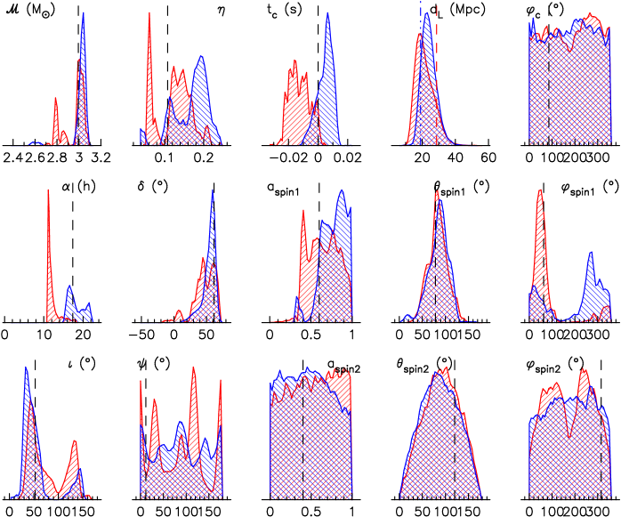
Figure 1: One-dimensional marginalised PDFs for all 15 parameters from our analysis of data sets DS1 (hatched upward; red in the online colour version) and DS2 (hatched downward; blue in the online colour version). The vertical dashed lines mark the injection values.

Table  1 shows the median and the width of the 95%-probability ranges for each parameter. The differences we find between the results for DS1 and DS2 may be attributed to the particular noise realisations in this example, and most parameters yield similar PDFs and accuracies.

Table 1: Median and width of the 95%-probability ranges for each parameter of the analyses of data sets DS1 and DS2. The column recovered indicates whether or not the 95% range includes the injection value.

• 		DS1 (synthetic noise)			DS2 (detector noise)
  	injection	median	95% width	recovered	median	95% width	recovered
  ${\cal M}\,(M_{\odot})$	2.99	3.006	0.294	yes	3.041	0.122	yes
  $\eta$	0.107	0.133	0.145	yes	0.183	0.144	yes
  $d_{\mathrm{L}}$ (Mpc)	28.615	21.240	20.764	yes	24.144	17.238	yes
  $t_{\mathrm{c}}$ (s)	0.000	-0.013	0.024	yes	0.006	0.019	yes
  $\phi_{\mathrm{c}}\,(^{\circ})$	85.944	189.745	342.398	yes	185.482	343.175	yes
  $\alpha$ (h)	17.380	11.684	5.349	no	17.786	6.320	yes
  $\delta\,(^{\circ})$	61.642	49.326	64.346	yes	58.390	39.796	yes
  $i\,(^{\circ})$	52.753	67.056	110.735	yes	46.850	122.787	yes
  $\psi\,(^{\circ})$	11.459	93.162	176.358	yes	88.706	173.869	yes
  $a_{\mathrm{spin1}}$	0.600	0.658	0.594	yes	0.804	0.478	yes
  $\theta_{\mathrm{spin1}}\,(^{\circ})$	78.463	85.490	83.110	yes	89.225	85.787	yes
  $\phi_{\mathrm{spin1}}\,(^{\circ})$	63.025	57.171	335.592	yes	263.014	345.700	yes
  $a_{\mathrm{spin2}}$	0.400	0.532	0.945	yes	0.475	0.940	yes
  $\theta_{\mathrm{spin2}}\,(^{\circ})$	120.000	94.687	150.544	yes	89.406	146.101	yes
  $\phi_{\mathrm{spin2}}\,(^{\circ})$	315.127	181.959	327.603	yes	184.681	339.071	yes
  $M_{1}\,(M_{\odot})$	10.002	8.533	8.849	yes	6.421	6.536	yes
  $M_{2}\,(M_{\odot})$	1.400	1.598	1.277	yes	2.036	1.564	yes

The PDFs of the parameters that describe the spin of the NS follow the prior distributions in both runs. This justifies ignoring the NS spin (by fixing $a_{\mathrm{spin2}}$ to 0.0 in the recovery template) for this mass ratio [2008ApJ...688L..61V]. For each of the two data sets, DS1 and DS2, we computed the Bayes factor to compare the evidence for the following two models: $M_{1}$: a ${3.5}$-pN inspiral waveform embedded in Gaussian noise, and $M_{2}$: Gaussian noise only. The values are listed in table  2. In both cases, the Bayes factor is large, providing strong evidence for a GW signal in the data. The difference in Bayes factor between DS1 and DS2 is attributed to an inherent spread due to different noise realisations, and the uncertainties of our method to estimate the Bayes factor (section 3). The results in this section show an illustrative example, but cannot be used to draw firm conclusions. However, it is clear that they warrant a larger, systematic study of these phenomena with the methods described here.

Table 2: Bayes factors $B_{1,2}$ between the models $M_{1}$: a ${3.5}$-pN inspiral waveform embedded in Gaussian noise, and $M_{2}$: Gaussian noise only (section 4.3) for data sets DS1 and DS2 (see section 4.1).

• 	DS1 (Gaussian noise)	DS2 (detector data)	DS3 (glitch)
  $\log_{e}B_{1,2}$	52.9	43.5	68.5

4.4 Analysis of data sets DS2 and DS3

On November 2nd 2006, seismic activity at Hanford and Livingston resulted in a coincident “glitch” in the data from the H1 and L1 LIGO detectors. These glitches were recovered by the Compact Binary Coalescence detection pipeline at an SNR of 11.3, using non-spinning, stationary-phase-approximation templates, Newtonian in amplitude and 2.0-pN in phase [2009PhRvD..79l2001A]. We defined the corresponding data set as DS3 in section 4.1 and analysed the data as if it had yielded a GW trigger. The convergence test from section 4.2 yields a 20% convergence rate, which results in our rejection of the results as not converged. However, when we nevertheless construct the marginalised one-dimensional PDFs from the data of the two converged chains (because of the small number of data points, the resulting PDFs may not be very accurate), they are similar in appearance to those from DS2 (see figure  2). The Bayes factors in table  2 even suggest that the data set DS3 is more consistent with containing a GW signal than DS2 (with the caveat that the SNRs of DS2 and DS3 were not computed the same way). On the other hand, the low value for the median of $\eta$ (0.05) corresponds to a mass ratio of 18, which is near the limit of the regime where post-Newtonian expansions are valid. In particular, a small value for eta suggests a slow frequency evolution which may indicate a spike in the frequency spectrum that dominates the signal. In addition, we find that the sky map for DS3 does not display the (parts of a) sky ring that is expected for an analysis using two non-co-located detectors 2009CQGra..26k4007Rsee e.g.. These results indicate that we should thoroughly verify our tests, such as the convergence criterion described here, using a large number of different glitches.

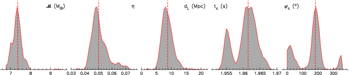
Figure 2: One-dimensional marginalised PDFs of a few selected parameters from our analysis of data set DS3. The vertical dashed lines indicate the median of each PDF.

5 Conclusions

We have developed the code SPINspiral which can do a complete parameter analysis of the gravitational-wave signals from quasi-circular compact-binary inspirals. We presented an example of the analysis of software injections into both simulated Gaussian noise (DS1) and LIGO-detector data (DS2). We also presented an analysis of a data set containing no injection, but a “glitch” coincident in two LIGO interferometers (DS3). These examples demonstrate a remarkable similarity between the results obtained from a GW signal injected in Gaussian noise and a similar signal in detector data. The Bayes factors are also similar, where we note that our present technique for computing the Bayes factor yields estimates with significant variance, and more precise estimates should be possible in the future. In addition, we find that although the Markov chains in the analysis of a coincident glitch in LIGO data do not converge, the resulting PDFs could look remarkably consistent with a simulated GW signal. We plan to run our code on a very large number of coincident triggers from the LIGO Compact Binary Coalescence search pipeline (noise events that are somehow being registered as resembling a binary inspiral) in order to get a good sense of how to distinguish them from actual inspirals. We conclude that further, detailed investigations are necessary to ensure we can rely on the robustness of our tests.

References

References

- [1] \harvarditemAbadie et al.20102010arXiv1003.2480L Abadie J, Abbott B P \harvardand al. 2010 ArXiv e-prints 1003.2480.
- [2] \harvarditemAbbott et al.2009a2009NJPh…11g3032A Abbott B, Abbott R \harvardand al. 2009a New Journal of Physics 11(7), 073032–+.
- [3] \harvarditemAbbott et al.2009b2009PhRvD..79l2001A Abbott B P, Abbott R \harvardand al. 2009b Phys. Rev. D 79(12), 122001.
- [4] \harvarditemAcernese et al.20082008CQGra..25r4001A Acernese F, Alshourbagy M \harvardand al. 2008 Class. Quant. Grav. 25(18), 184001–+.
- [5] \harvarditemApostolatos et al.19941994PhRvD..49.6274A Apostolatos T A, Cutler C, Sussman G J \harvardand Thorne K S 1994 Phys. Rev. D 49, 6274–6297.
- [6] \harvarditemAtchadé \harvardand Rosenthal2005atchade_rosenthal_2005 Atchadé Y F \harvardand Rosenthal J S 2005 Bernoulli 11(5), 815–828.
- [7] \harvarditemBuonanno et al.20032003PhRvD..67j4025B Buonanno A, Chen Y \harvardand Vallisneri M 2003 Phys. Rev. D 67(10), 104025.
- [8] \harvarditemCutler \harvardand Flanagan19941994PhRvD..49.2658C Cutler C \harvardand Flanagan É E 1994 Phys. Rev. D 49, 2658–2697.
- [9] \harvarditemCutler \harvardand Thorne20022002gr.qc…..4090C Cutler C \harvardand Thorne K S 2002 Proceedings of GR16, World Scientific, Singapore .
- [10] \harvarditemEarl \harvardand Deem2005earl-2005 Earl D J \harvardand Deem M W 2005 ArXiv e-prints physics/0508111.
- [11] \harvarditemFigueiredo \harvardand Jain2002figueiredo_jain_2002 Figueiredo M A T \harvardand Jain A K 2002 IEEE Transactions on pattern analysis and machine intelligence 24(3), 381–396.
- [12] \harvarditemGelman et al.1997gelman_etal_1997 Gelman A, Carlin J B, Stern H \harvardand Rubin D B 1997 Bayesian data analysis Chapman & Hall, Boca Raton.
- [13] \harvarditemGilks et al.1996gilks_etal_1996 Gilks W R, Richardson S \harvardand Spiegelhalter D J 1996 Markov chain Monte Carlo in practice Chapman & Hall/CRC.
- [14] \harvarditemHansmann19971997CPL…281..140H Hansmann U 1997 Chemical Physics Letters 281, 140–150.
- [15] \harvarditemHukushima \harvardand Nemoto19961996JPSJ…65.1604H Hukushima K \harvardand Nemoto K 1996 Journal of the Physical Society of Japan 65, 1604.
- [16] \harvarditemJaranowski \harvardand Krolak19941994PhRvD..49.1723J Jaranowski P \harvardand Krolak A 1994 Phys. Rev. D 49, 1723–1739.
- [17] \harvarditemLIGO Scientific Collaboration2007LAL LIGO Scientific Collaboration 2007 The LSC Algorithm Library. https://www.lsc-group.phys.uwm.edu/daswg/projects/lal.html.
- [18] \harvarditemNewton \harvardand Raftery19941994JSTOR..N Newton M A \harvardand Raftery A E 1994 JRSS B 56(1), 3–48. http://www.jstor.org/stable/2346025.
- [19] \harvarditemO’Shaughnessy et al.20082008ApJ…672..479O O’Shaughnessy R, Kim C, Kalogera V \harvardand Belczynski K 2008 ApJ 672, 479–488.
- [20] \harvarditemPoisson \harvardand Will19951995PhRvD..52..848P Poisson E \harvardand Will C M 1995 Phys. Rev. D 52, 848–855.
- [21] \harvarditemRaymond et al.20092009CQGra..26k4007R Raymond V, Van der Sluys M V, Mandel I, Kalogera V, Röver C \harvardand Christensen N 2009 Classical and Quantum Gravity 26(11), 114007.
- [22] \harvarditemRöver20072007PhD..Auck Röver C 2007 Bayesian inference on astrophysical binary inspirals based on gravitational-wave measurements PhD thesis The University of Auckland. http://hdl.handle.net/2292/2356.
- [23] \harvarditemRöver et al.20062006CQGra..23.4895R Röver C, Meyer R \harvardand Christensen N 2006 Class. Quant. Grav. 23, 4895–4906.
- [24] \harvarditemRöver et al.20072007PhRvD..75f2004R Röver C, Meyer R \harvardand Christensen N 2007 Phys. Rev. D 75(6), 062004.
- [25] \harvarditemSkilling2006MR2282208 Skilling J 2006 Bayesian Anal. 1(4), 833–859 (electronic).
- [26] \harvarditemVan den Broeck \harvardand Sengupta20072007CQGra..24.1089V Van den Broeck C \harvardand Sengupta A S 2007 Class. Quant. Grav. 24, 1089–1113.
- [27] \harvarditemVan der Sluys et al.20082008CQGra..25r4011V Van der Sluys M, Raymond V, Mandel I, Röver C, Christensen N, Kalogera V, Meyer R \harvardand Vecchio A 2008 Class. Quant. Grav. 25(18), 184011.
- [28] \harvarditemVan der Sluys \harvardand al.in preparationvandersluysprep Van der Sluys M V \harvardand al. in preparation.
- [29] \harvarditemVan der Sluys et al.20082008ApJ…688L..61V Van der Sluys M V, Röver C, Stroeer A, Raymond V, Mandel I, Christensen N, Kalogera V, Meyer R \harvardand Vecchio A 2008 ApJ 688, L61–L64.
- [30] \harvarditemVan Haasteren2009vanhaasteren-2009 Van Haasteren R 2009 ArXiv e-prints 0911.2150.
- [31] \harvarditemVeitch \harvardand Vecchio2008a2008CQGra..25r4010V Veitch J \harvardand Vecchio A 2008a Classical and Quantum Gravity 25(18), 184010.
- [32] \harvarditemVeitch \harvardand Vecchio2008b2008PhRvD..78b2001V Veitch J \harvardand Vecchio A 2008b Phys. Rev. D 78(2), 022001.
- [33] \harvarditemVeitch \harvardand Vecchio20092009arXiv0911.3820V Veitch J \harvardand Vecchio A 2009 ArXiv e-prints 0911.3820.
- [34] \harvarditemWillke et al.20042004CQGra..21S.417W Willke B, Aufmuth P \harvardand al. 2004 Class. Quant. Grav. 21, 417.
- [35]