A reduction method for noisy Boolean networks
Abstract
This paper is concerned with the reduction of a noisy synchronous Boolean network to a coarse-grained Markov chain model. Consider an -node Boolean network having at least two basins of attraction and where each node may be perturbed with probability during one time step. This process is a discrete-time homogeneous Markov chain with possible states. Now under certain conditions, the transitions between the basins of the network may be approximated by a homogeneous Markov chain where each state of the chain represents a basin of the network, i.e. the size of the reduced chain is the number of attractors of the original network.
1Affiliation: Montefiore Institute, Department of Applied Mathematics, University of Liège, B28, B-4000 Liège, Belgium
2Affiliation: Algology, Mycology and Experimental Systematics, Department
of Life Sciences, University of Liège, B22, B-4000 Liège, Belgium
1 Noisy Boolean networks (NBNs)
1.1 Definition
Boolean networks (BNs) have been used for several decades as models of biochemical networks, mainly to predict their qualitative properties and, in the case of genetic regulatory networks, to infer the inputs and interaction rules of their nodes from microarray data (Kauffman,, 1969; Glass and Kauffman,, 1973; Kauffman,, 1993; Li et al.,, 2004; Martin et al.,, 2007; Samal and Jain,, 2008).
An -node BN model consists of interacting nodes which, in the context of biochemical networks, generally represent genes or molecular species such as proteins, RNAs or metabolites. Let denote the Boolean variable describing the state of node at discrete time If node represents a protein, then we say that if the value of the node is , then the protein is present, in its active form and its target (or substrate) present. Using De Morgan’s law, the negation of this conjunction gives the interpretation for value : the protein is absent or inactive or its target (or substrate) absent.
Remark 1
A more concise interpretation instead of “present” (resp. “absent”) is “present and not being degraded” (resp. “absent or being degraded”) or even “present and production rate greater than degradation rate” (resp. “absent or degradation rate greater than production rate”).
For an -node synchronous BN, the interactions between the nodes are modeled by a set of Boolean interaction functions such that:
| (1) |
with interaction function of node . If the state of node at time depends on the state of node at previous time , then node is said to be an input for node . The number of inputs of a node is called the connectivity of that node. The network is said to be synchronous because as expressed in (1) the nodes are updated synchronously. Also from (1) the dynamics of the network deterministic.
Let us take an example to illustrate some essential properties of BNs. Consider the following BN:
| (2) |
where symbols , and represent logical operators NOT, OR and AND respectively. The size of the state space of this network, i.e. the number of possible states, is since here. From (1.1), the next state for each possible state can be computed to obtain the state table of the network. Using this state table then, the state diagram can be built. This is shown in Fig 1 where it can be seen that the state space has been partioned into two disjoint sets. These sets are called basins of attraction and are denoted by B1 and B2 in the figure. Each basin consists of an attractor and some transient states. The attractor of B1 is the fixed point : whatever the initial state in B1, the network will converge to and stay there forever. Attractors may also be periodic as is the case for basin B2. The size of a basin or of an attractor is the number of states that constitute it.
Now suppose that, due to random perturbations, each node of a BN has probability to switch its state ( to or vice versa) between any two times and . Then we get a noisy BN (NBN)111Here, for the sake of simplicity, perturbation probability is supposed to be independent of time and of the states of the nodes. If, for instance, for a particular node, to random switching probability is set greater than to one, then it means that random perturbations tend to turn the node ON rather than OFF.. The introduction of disorder is supported by the stochastic nature of intracellular processes coupled to the fact that, thermodynamically speaking, biochemical networks are open systems.
One important difference between a BN and a NBN is that in the latter, transitions between the basins of the network are allowed. For example, in the state diagram of Fig. 1, if we perturb simultaneously nodes and of attractor state which is in B1, then we go to transient state which belongs to B2.
Remark 2
Flipping the value of single nodes has been envisaged by Kauffman, (1993) in genetic Boolean networks to study their stability to what he called minimal perturbations. Shmulevich et al., (2002) proposed a model for random gene perturbations based on probabilistic Boolean networks (a class of Boolean networks that enclosed the class of synchronous Boolean networks by assigning more than one interaction function to each node) in which any gene of the network may flip with probability independently of other genes and interpreted the perturbation events as the influence of external stimuli on the activity of the genes.
Let be the probability that exactly nodes will be perturbed during one time step. Then letting :
| (3) |
This is the binomial probability distribution with parameters and . On average, nodes are perturbed at each time step. The probability that at least one node will be perturbed during one time step is therefore:
| (4) |
Since we are mainly interested in the behaviour of the network as varies, in the following and will be considered as parameters while will be considered as a variable. Thus we should write instead of 222 is a function of with parameters and . It is not a probability density function. For fixed , is a probability..
For , has a maximum at and .
The Maclaurin series of up to order is:
Thus one has:
| (5) |
This means that, being fixed, for sufficiently small the probability that nodes be perturbed during one time step is negligible compared to the probability that just one node be perturbed. Table 1 gives some values of rounded to four decimal places. We see that at , and .
| 0.002 | 0.02 | 0.2 | 0.5 | |
|---|---|---|---|---|
| 0.0080 | 0.0753 | 0.4096 | 0.2500 | |
| 0.0000 | 0.0023 | 0.1536 | 0.3750 | |
| 0.0000 | 0.0000 | 0.0256 | 0.2500 | |
| 0.0000 | 0.0000 | 0.0016 | 0.0625 | |
| 0.0158 | 0.1389 | 0.3355 | 0.0312 | |
| 0.0001 | 0.0099 | 0.2936 | 0.1094 | |
| 0.0000 | 0.0004 | 0.1468 | 0.2188 | |
| 0.0000 | 0.0000 | 0.0459 | 0.2734 | |
1.2 The mean specific path
Consider a series of Bernoulli trials where each time step defines one trial and where a success means that at least one node has been perturbed. From (4), the probability that the first success will occur on trial is:
| (6) |
which is a geometric distribution with parameter . The first moment of this distribution (the mean time between two successes) is:
| (7) |
We see that is a decreasing function of and , that tends to as and to as . Since time step is unity, equals the mean number of state transitions between two successes. By analogy with the mean free path of a particle in physics333In kinetic theory of gases, the mean free path of a gas molecule is the mean distance traveled by the molecule between two successive collisions., will be called mean specific path. The term “specific” is used to recall that between two successes, the trajectory in the state space is specific to node interactions, i.e., it is entirely determined by node interactions.
For sufficiently small one has , where the last approximation comes from (5). Hence, for sufficiently small we may write:
Depending on the value of , different dynamical regimes are possible. For , the network is trapped by an attractor where it stays forever. For , transitions between the basins of the network occur. The more is close to one, the shorter the times spent on the attractors, the more the network suffers from functional instability. In the low regime, the network may both maintain a specific activity for a long time period and change its activity: functional stability and flexibility (or diversity) coexist.
1.3 Time evolution equation
A NBN is in fact a discrete-time Markov chain , where is the random variable representing the state of the network at time . The state space of an -node BN will be denoted by , with and with state corresponding to binary representation of .
Let be the conditional probability that the network will be in state at while in state at . The matrix of size whose elements are the ’s will be denoted by and is called the transition probability matrix in Markov theory. The sum of elements in each row of is unity. Let be the probability that the network will be in state at time and denote by the vector whose elements are the state probabilities . Given an initial state probability vector , the vectors are found from (Kleinrock,, 1975):
| (8) |
Matrix is the sum of two matrices:
-
1.
The perturbation matrix , whose th element is equal to
where refers to th element of Hamming distance matrix , a symmetric matrix that depends only on . Element is equal to the number of bits that differ in the Boolean representations of states and . Diagonal elements of are therefore . For example, if , takes the form:
-
2.
The interaction matrix . If the node interactions are such that starting in state the network is forced to transition to state in one time step, then th element of equals , otherwise it is . Notice that if th diagonal element of equals then state is a fixed point (attractor of size ).
Therefore, for fixed , any probability will be either or a function of .
1.4 Stationary probability distribution
Since does not depend on , the ’s are independent of time. The chain is thus homogeneous. As shown by Shmulevich et al., (2002) for genetic probabilistic Boolean networks, for , the chain is irreducible and aperiodic. Consequently, for given there is a unique stationary distribution which is independent of (Kleinrock,, 1975). The stationary distribution satisfies the two equations:
| (10) |
In addition, we have:
| (11) |
where each row of is equal to vector .
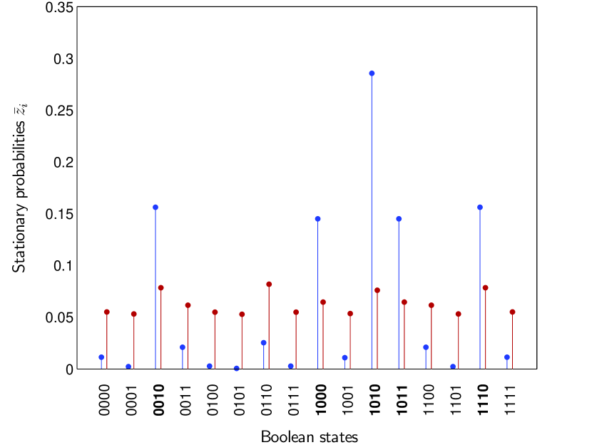
Fig. 2 shows the stationary state probabilities for the network of Fig. 1 and two values. Blue points correspond to and red ones to . As can be seen in the figure, when , the stationary probabilities of the transient states are small compared to those of the attractor states (attractor states are represented in bold type in the figure). Therefore in the low regime, the activity of the network in the long term is governed mostly by its attractors444Equivalently, in the low regime, it is mostly attractors that determine the fate of the cells.. In fact, the stationary probabilities of the transient states tend to as tends to . Also notice for the stationary probabilities of the second attractor almost equal.
As tends to unity, the stationary probabilities tend to be uniform, i.e. as one has (see the case ). Thus for sufficiently close to unity, the stationary probabilities of the transient states are not negligible compared to those of the attractor states.
Remark 3
For sufficiently small , the stationary probability of an attractor state may be approximated by where is the limit as of the stationary occupation probability of the basin containing the attractor and the size of the attractor (see further 4.3). Thus in the case of the network of Fig. 1, we get for attractor state (fixed point) that , and for the states of the second attractor, that each stationary state probability .
2 Method for the calculation of the sojourn time distribution in a basin of a NBN
Consider a BN having at least two basins. Consider a basin B of size of this network and a fixed perturbation probability . Let
| (12) |
The square sub-matrix contains the one-step transition probabilities between the states of B. For example, in the case of basin B1 of Fig. 1, element of is equal to the one-step transition probability between state () and state (). Element of vector represents the one-step transition probability between state and an absorbing state555A state such that once reached, it is not possible to escape from it. regrouping states , i.e.
is a row vector of length with all elements zero and is a scalar.
From matrix , we can calculate the probability that the network will be in basin B at time given an initial probability vector of length with sum of elements :
| (13) |
and by definition:
with .
Now we want the sojourn time distribution in B. We shall denote by the discrete random variable representing the sojourn time in B, with sample space , and by the probability distribution of , i.e. . For a given basin, depends on and initial vector . It is given by:
| (14) |
while the cumulative distribution function of is:
| (15) |
Matrix in (12) represents an absorbing Markov chain (Snell,, 1959), i.e. it has at least one absorbing state and from every non-absorbing state (every state ) one can reach an absorbing state (any state ). If the chain is initially in state , then the mean time spent in state before absorption is the th element of fundamental matrix (Snell,, 1959). Thus if denotes the mean of then:
| (16) |
Here is a column vector of length with each element .
Also notice from the definitions of the mean of and of that can be expressed as follows:
3 The problem of geometric approximation
Let be a geometric distribution with parameter , i.e. and have same mean. Consider the maximum deviation between the cumulative distribution functions (cdfs) of these two distributions, namely:
| (17) |
with and the cdf of , i.e. , In probability theory, is called the Kolmogorov metric. As , is not defined for and, for a given basin, depends on and . It comes from (15) that:
| (18) |
Thus represents the absolute error between and its geometric approximation . For basins of size (one fixed point and no transient states), is given by (6) which is geometric. Hence for such basins and thus . This is a particular case and in the following we shall study the behaviour of as tends to without any assumptions on .
The probability to exit B during is:
| (19) |
This probability depends on , and . In particular, for , is constant and equal to . When , any state communicates with any state , thus and therefore probability is strictly decreasing.
Inversely, since , we have:
| (20) |
and thus
| (21) |
We see that if then . Also note the following:
-
1.
(22) Whatever the initial conditions, as becomes smaller, it takes on average more and more time to leave the basin. Also this means that : as .
-
2.
(23) Whatever and the initial conditions, the probability to leave the basin during goes to as . Indeed, from equations (13) and (19), it comes that
(24) with the number of ways of leaving B by perturbing bits of state 666This number is equal to the number of elements in row of the Hamming distance matrix that are equal to and whose column index is such that . and
i.e.
In order to show that any tends to as tends to , we introduce two propositions.
Proposition 1
For any basin of a noisy Boolean network with fixed , the fundamental matrix has a real simple eigenvalue which is greater in modulus than any other eigenvalue modulus, that is for any other eigenvalue of . We have:
For a given basin, the rate of convergence depends on and while the limit depends only on .
From that proposition, we see that if is geometric then . For example, if then .
Demonstration.
We have to show that:
with a real simple eigenvalue of greater in modulus than any other eigenvalue modulus and .
Matrix is nonnegative. It is irreducible and aperiodic thus primitive. From the Perron-Frobenius theorem, we have that: (1) has a real eigenvalue which is greater in modulus than any other eigenvalue modulus. Since is substochastic, we have . (2) is a simple root of the characteristic equation of . Moreover (Douglas and Brian,, 1999):
with and right and left eigenvectors associated with chosen in such a way that , and . The greater , the better the approximation . Thus:
Therefore:
Proposition 2
is asymptotically equivalent to :
Since does not depend on , the last statement is equivalent to say that as tends to , is less and less dependent on . In other words, from (16), the elements of vector tends to be equal as .
Demonstration.
If is geometric then does not depend on . Thus from (16) it comes that:
or equivalently
| (25) |
This means that is an eigenvalue of with associated eigenvector . Since is nonnegative primitive, by the Perron-Frobenius theorem, must equal , which implies . Now . Thus . From (25) we see that the sum of elements in any row of is a constant. This is because when is geometric, the probability to leave the basin from any state is constant.
When is not geometric, the Perron-Frobenius theorem gives:
Now as tends to , tends to a stochastic matrix (because vector tends to vector null). Therefore as tends to , must tend to and must tend to . Thus for sufficiently small we may write:
| (26) |
or equivalently
Therefore
Thus as , will be less and less dependent on initial conditions and the error in the above approximation will tend to . Note that since as we must have as which is result (22).
Remark 4
As will be discussed later, approximation may be good in some neighborhood of some (typically in the neighborhood of , see Fig. 13 in 4.3).
From Proposition 2 now, will tend to as . On the other hand, from (26), we get
and thus:
Hence from (18) any will tend to as tends to , whatever . Thus the maximum will do so:
Since the maximum deviation between the two cdfs of and vanishes as , these two cdfs tend to coincide as p tends to . Also this means that is a good approximation to within of at any and every and that the error can be made arbitrarily small by taking sufficiently close to (but not equal to ).
In addition, from (22) we may write for sufficiently small :
Yet the cdf of an exponential distribution with parameter is:
For and , the two probabilities are equal. Therefore, as and , the cdf of tends to coincide with the cdf of an exponential distribution. Since is less and less dependent on as (see Proposition 2), one has for sufficiently small that an exponential distribution can be used to approximate the time spent in a basin of a NBN.
Remark 5
Depending on , may be very close to a geometric distribution while is not small. See Examples 1 and 2 below.
Suppose that for each basin of a NBN the sojourn time is sufficiently memoryless. Then, under some additional assumptions that will be discussed in section 5, one may define another discrete-time homogeneous Markov chain whose states are the basins of the network. (1) This new stochastic process is coarser than since only transitions between the basins of the network are described. (2) The size of its state space is in general much smaller than , the size of the state space of the original process. (3) It has to be viewed as an approximation. The tilde symbol in is used to recall that in general, a basin does not retain the Markov property (i.e., is not geometric).
Example 1
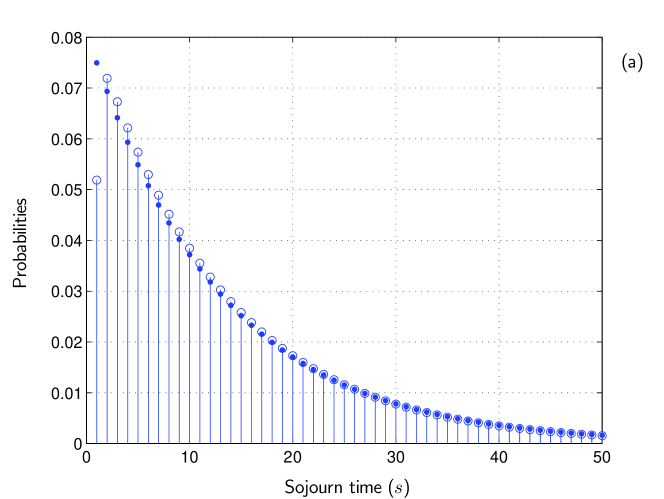
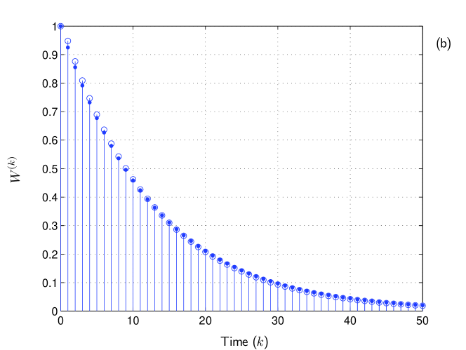
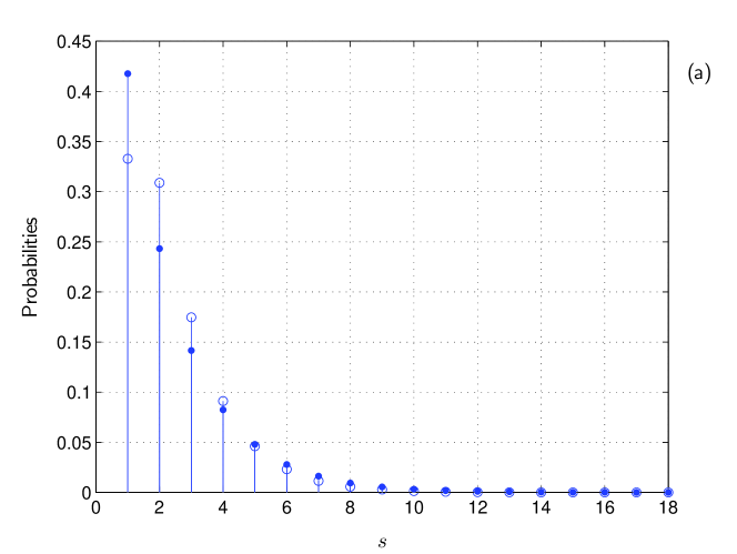
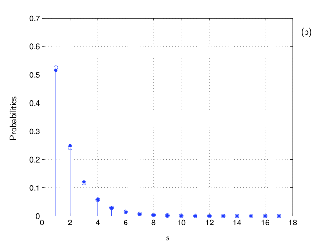
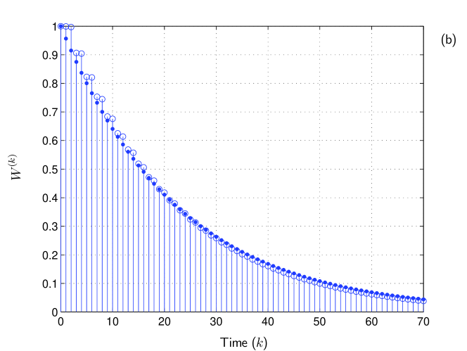
Calculation of sojourn time distributions and illustration of the geometric approximation problem. Let us take basin B1 of Fig. 1 with and , and let us compute and . The two distributions are plotted in Fig. 3a. The circles stand for the probabilities (), the points for the probabilities (). Fig. 3b shows and its geometric approximation versus time . Maximum deviation between the two is .
Table 2 gives and for different values and different initial conditions for the two basins of Fig. 1. Each of the four columns below and corresponds to one value, from left to right: , , and . The mean values of the columns are also given (see the rows with “Mean”). For the calculation of , we considered two types of initial conditions: (1) the network starts in one state of the basin (successively each state of the basin was taken as initial state) and (2) (see “Unif.” in the Table). We see that for the first three values of the mean sojour times in B1 are smaller than those in B2 (see the first three columns below ). Thus B1 is less stable than B2. Also calculated for each basin and the four values the variation coefficient of the sojourn times obtained with the first type of initial conditions. The results are (columns , , and ): , , and for B1; , , and for B2. Therefore is less and less sensitive to the initial state as decreases, which is in accordance with Proposition 2.
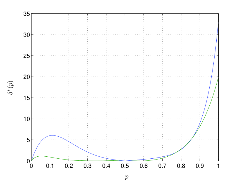
Another important observation in this table is that, depending on the initial conditions, may be close to a geometric distribution while is not small (see in the table the values of when ). Fig. 4 shows the functions for the two basins of Fig. 1 and the uniform initial condition. We see that in both cases when , ( is geometric at )777Whatever the initial conditions, at , for B1 and for B2. See 5.1.2 for analytical expression of when . and tends to a global maximum as . For basin B1 (blue curve), there is one local maximum at , while for basin B2 (green curve) there are two local maxima, one at and the other at , and one local minimum at (). As mentioned above, function depends on initial conditions. For example, if the network starts in state , then B2 has still one local minimum but this now occurs at ().
| Ini. cond. | |||||||||
|---|---|---|---|---|---|---|---|---|---|
| B1 | 126.00 | 13.52 | 2.37 | 1.54 | 0.39 | 3.44 | 7.47 | 10.39 | |
| 126.00 | 13.52 | 2.39 | 2.07 | 0.39 | 3.47 | 8.49 | 4.09 | ||
| 125.50 | 13.02 | 1.94 | 2.28 | 0.00 | 0.00 | 0.92 | 10.66 | ||
| 126.00 | 13.52 | 2.39 | 2.07 | 0.39 | 3.47 | 8.49 | 4.09 | ||
| 125.50 | 13.02 | 1.94 | 2.28 | 0.00 | 0.00 | 0.92 | 10.66 | ||
| 126.00 | 13.52 | 2.37 | 1.54 | 0.39 | 3.44 | 7.47 | 10.39 | ||
| Mean | 125.83 | 13.35 | 2.23 | 1.96 | 0.26 | 2.30 | 5.63 | 8.38 | |
| Unif. | 125.83 | 13.35 | 2.23 | 1.96 | 0.26 | 2.30 | 4.59 | 2.72 | |
| B2 | 252.85 | 27.68 | 4.27 | 3.77 | 0.39 | 2.96 | 2.31 | 5.40 | |
| 251.86 | 26.81 | 4.08 | 2.25 | 0.00 | 0.11 | 0.50 | 20.87 | ||
| 252.36 | 27.26 | 4.22 | 3.77 | 0.20 | 1.63 | 2.59 | 5.42 | ||
| 251.86 | 26.80 | 4.02 | 3.60 | 0.00 | 0.12 | 1.99 | 0.93 | ||
| 251.86 | 26.80 | 4.02 | 3.60 | 0.00 | 0.12 | 1.99 | 0.93 | ||
| 251.86 | 26.80 | 4.02 | 3.60 | 0.00 | 0.12 | 1.99 | 0.93 | ||
| 251.86 | 26.80 | 4.02 | 3.60 | 0.00 | 0.12 | 1.99 | 0.93 | ||
| 252.36 | 27.26 | 4.22 | 3.77 | 0.20 | 1.63 | 2.59 | 5.42 | ||
| 251.86 | 26.81 | 4.08 | 2.25 | 0.00 | 0.11 | 0.50 | 20.87 | ||
| 252.85 | 27.68 | 4.27 | 3.77 | 0.39 | 2.96 | 2.31 | 5.40 | ||
| Mean | 252.16 | 27.07 | 4.12 | 3.40 | 0.12 | 0.99 | 1.88 | 6.71 | |
| Unif. | 252.16 | 27.07 | 4.12 | 3.40 | 0.12 | 0.81 | 0.24 | 2.81 | |
Example 2
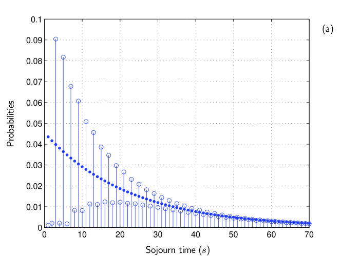
In this example, we illustrate the fact that while is not small, may be close to a geometric distribution, depending on . We take basin B1 of Fig. 1 and calculate when initially the network is (a) in state and (b) in state . Fig. 5 shows the results. As can be seen in the figure, when the network starts in , is close to a geometric distribution which is not the case when the initial state is .
To compare the two approximations, we computed the variances and of and respectively and the total variation distance between and (another probability metric) which is given by:
The values of these parameters are given in Table 3. We see that the total variation distance is about times greater when the initial state is than when it is . The more geometric , the smaller , the better the approximations and .
| (%) | 8.49 | 0.92 |
|---|---|---|
| (%) | 10.75 | 1.18 |
| 2.38 | 1.91 | |
| 3.34 | 1.82 | |
| 2.00 | 2.00 | |
| 2.39 | 1.94 |
Till now, we have assumed each node of the network has the same probability of being perturbed. In Example below, we look at how the network of Fig. 1 behaves when one of its nodes is perturbed with a probability which is high compared to the other nodes. Suppose nodes represent proteins. Within the cell interior, some proteins may be more subject to competing reactions than others. These reactions may be assumed to act randomly888Due to the fluctuating nature of intracellular processes., either negatively or positively, on the state of the target proteins. For example, some reactions may lead to protein unfolding while others, like those involving molecular chaperones, may rescue unfolded proteins (Dobson,, 2003). On the other hand, some proteins may be more sensitive to physico-chemical factors, like temperature or pH, increasing their probability to be perturbed.
Example 3
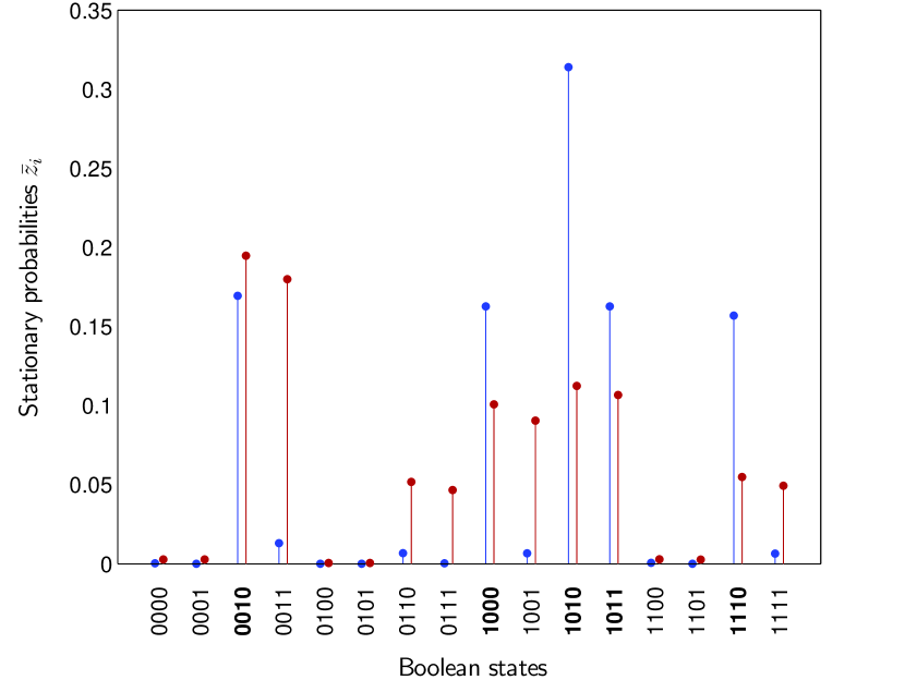
In this example, it is assumed that one node is perturbed with a probability which is high compared to the other nodes. The behaviour of the network when is complex and will not be discussed here so we take (the first three nodes are rarely perturbed) and . Fig. 6 shows for two values of . For (the blue points) the network behaves as if all the nodes had the same probability of being perturbed (see Fig. 2, the blue points). Simulations have shown this to be true whatever the three rarely perturbed nodes. When increases in , the stationary state probabilities do not tend to be equal (see Fig. 6, the case ), rather, some transient states, typically state of B2, tend to be more populated at the expense of attractor states (see attractor states , , and in Fig. 6)999At the cell population level, this means that a cell population would exhibit phenotypes that could not have been observed (or not easily observed) in the low regime. Note that these phenotypes are not necessarily survivable for the cells..
4 The geometric approximation in networks
In Example 1, we illustrated, using the network of Fig. 1, the fact that as tends to , the cdf of the time spent in a basin of attraction approaches the cdf of a geometric (resp. exponential) distribution and that the expected sojourn time tends to be independent of initial conditions (see the decreases of and variation coefficient as becomes smaller, respectively in Table 2 and in the text). As will be seen later, for this network, a two-state discrete-time (resp. continuous-time) homogeneous Markov chain may be used for approximating basin transitions in the low regime, i.e., a coarse-grained description of this network exists in the low regime.
Now we address the problem of geometric approximation in randomly constructed networks. A random network is built by randomly choosing for each node inputs and one interaction function (Kauffman,, 1993).
4.1 networks and confidence intervals
Six ensembles were examined taking , or (, or ) and or . Each basin of a randomly constructed network was perturbed with , , , , , and .
According to the classification of Kauffman, (1993), networks are complex while ones are chaotic. One difference between these two ensembles of networks, which is of particular interest here, is that in the former “If the stability of each state cycle attractor is probed by transient reversing of the activity of each element in each state of the state cycle, then for about to percent of all such perturbations, the system flows back to the same state cycle. Thus state cycles are inherently stable to most minimal transient perturbations.” (Kauffman,, 1993, p. 201). In chaotic networks, the stability of attractors to minimal perturbations is at best modest (Kauffman,, 1993, p. 198).
For each ensemble, we generated about basins (which corresponds to about to networks depending on the ensemble). We established confidence intervals for three statistical variables of which two are probabilities:
-
1.
Consider an -node network. For each of its basins, one can define two conditional probabilities: (1) the conditional probability of leaving the basin given that one attractor bit out of has been flipped, with the size of the attractor, and (2) the conditional probability of leaving the basin given that one basin bit out of has been flipped.
In each basin sample, a small proportion of basins having were found. The th percentile of the relative size of basins was more than for networks and for ones. Thus basins are most often big basins. We calculated ratios: ratio between the median mean sojourn times of and basins and ratio between the maximum mean sojourn times of the two types of basins. These ratios are given in Table 4 for networks and four values. In the case of basins, the computation of for and stopping criterion varies between a few minutes to several days using a PowerEdge 2950 server with Quad-Core Intel Xeon processors running at 3.0 GHz. As can be seen from this table, with decreasing, the maximum mean sojourn time of basins increases drastically compared to that of basins101010For basins, the conditional probability of leaving the basin given that bits of an attractor state have been perturbed may be non null. However for . On the other hand, for transient states and sufficiently large one has as .. The proportion of basins varies in our samples from to depending on the ensemble. For fixed , it is a decreasing function of and for fixed , it is smaller in the chaotic regime than in the complex one. Although we do believe that basins have not to be rejected from a biological interpretation perspective, networks with at least one basin were omitted during the sampling procedure (essentially because of the high computational time that is needed to compute when and is small).
0.03 0.05 0.1 0.5 30.1612 19.9012 12.1390 6.8534 44.3541 26.0081 15.1438 11.9929 35.5351 21.6376 14.5090 10.3930 122.3414 19.3446 3.6270 1.0000 300.3482 32.4353 3.1643 1.0000 542.8109 67.3100 4.9887 1.0000 Table 4: Comparison between median mean sojourn times of and basins (ratio ) and between maximum mean sojourn times of both types of basins (ratio ) for networks and four values. Calculation of : at time , the states of the basin are equiprobable. The proportions of basins for samples , and were found to be , and respectively. 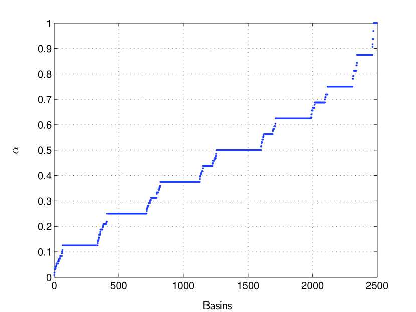
Figure 8: Conditional probabilities sorted in ascending order, sample . About of the data points are in main probability levels. These correspond to probabilities . Fig. 8 shows the conditional probabilities for sample . For an -node network, one can define main probability levels corresponding to probabilities . The percentage of data points located in main probability levels are given in Table 5 for the six samples and the two conditional probabilities and . It can be seen from this table that whatever the connectivity and the conditional probability, this percentage decreases when increases. For a given conditional probability and any , it is greater in the complex regime than in the chaotic one.
The statistical analysis of the six data samples has shown the following. For , there is a clear quantization of and a weak one of . Also the histograms of and are symmetric (skewness equal to ). For , the quantization of is weak and there is no obvious quantization of . The histograms of and are negatively skewed (skewness equal to ) and the last two main probability levels and are strongly populated compared to the other ones.
78.6 52.0 73.9 45.9 70.2 35.3 56.6 31.5 50.8 23.5 43.6 15.4 Table 5: Percentages of data points located in main probability levels for the six ensembles and the two conditional probabilities and . Table 6 gives the mean and median of probabilities and for the six ensembles . For fixed , the mean and median of both conditional probabilities are higher for chaotic basins than for complex ones. Additionally, for basins, the mean and median decrease with while for , both increase with (except for the median of ).
Mean Median Mean Median 0.5057 0.5000 0.4817 0.5000 0.4523 0.4375 0.4294 0.4144 0.4149 0.4000 0.3907 0.4000 0.6869 0.7917 0.6852 0.7778 0.7032 0.8125 0.7038 0.8219 0.7050 0.8125 0.7106 0.8375 Table 6: Mean and median of conditional probabilities and for the six ensembles . -
2.
The third statistical variable is the mean time spent in a basin, . For and any , there is a clear quantization at which rapidly disappears as increases. For and any , there are only two levels of quantization at and these rapidly vanish as increases. Also notice that the minimum of is equal to the mean specific path which, according to (7), does not depend on .
Most of the limits of the confidence intervals ranged between and (for and : confidence interval for the mean if , for the median and for the trimmed mean if ; for : confidence interval for the trimmed mean)111111Two methods were used: a nonparametric method based on the binomial distribution (for the median only) and the bootstrap method (used for the median and the trimmed mean). For the trimmed mean, we averaged the sample data that were (1) between the th and th percentiles, (2) less than the th percentile and (3) less than the th percentile..
4.2 Simulation results and discussion
Most of the basin variables (such as or ) were positively skewed. Therefore for each of these variables we calculated quartiles , (the median) and .
For the calculation of , two types of initial conditions were considered:
-
1.
Each element of is equal to . We call this condition the uniform initial condition.
-
2.
We pick one state of the basin at random and place initially the network in that state (the elements of are all except one which is equal to ). We call this condition the random initial condition.
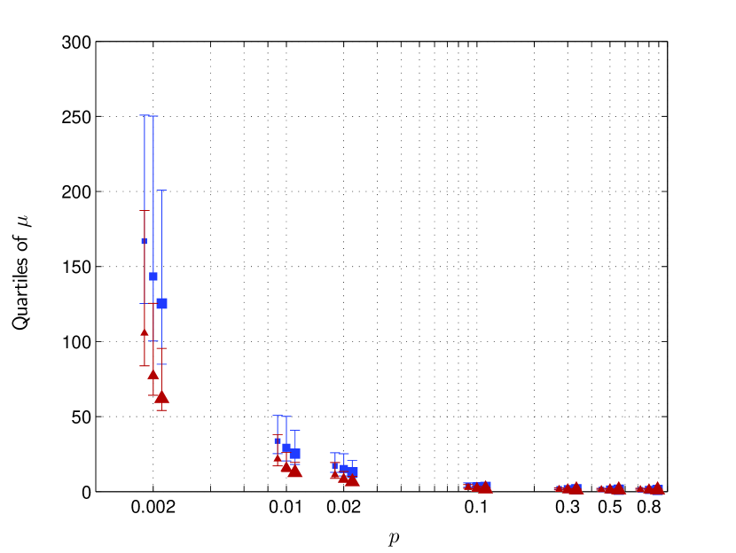
Let’s start with the basin variable . First the uniform initial condition. Coefficients of skewness for distributions mostly ranged from to with mean of (strong skewness). For example, for sample with , we obtained a coefficient of skewness of , a mean of , a median of , a th percentile of , a th percentile of and a maximum of . A small proportion of the mean sojourn times are therefore very far from the median (taken here as the central tendency). The three quartiles of versus are shown in Fig. 9 for the six ensembles . The blue squares correspond to and the red triangles to . The size of a symbol is proportional to . For the sake of clarity, the abscissæ of the points corresponding to ensembles and have been translated (respectively to the left and to the right of the values).
It can be seen from Fig. 9 that: (1) for fixed and any , the median of is a decreasing function of the size of the network (not true at and ), although decreases with (see Table 6). (2) For fixed and any , the median of is a decreasing function of . (3) For fixed and any , median of chaotic basins () is less than that of complex ones (). At , the medians of for ensembles are respectively , and times smaller than those for ones. Similar but smaller values were found for and . We therefore confirm the results of Kauffman, (1993, p. 198, 201 and 488-491) that chaotic basins are less stable to node perturbations than complex ones.
We looked for the relationship between the median of and . We found that for sufficiently small :
| (27) |
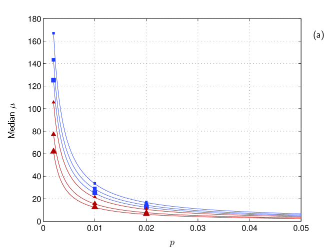
i.e. the median of the mean sojourn time is inversely proportional to . The proportionality constant has been estimated by the least squares method for the six ensembles and was found to decrease when increases (only the first three data points were fitted, i.e. the points with abscissa , and ). For , we obtained , and ; for , , and . Thus for fixed , chaotic basins are less sensitive to a variation in than complex ones. The result of the least squares fit is presented in Fig. 10. Graph (a) shows the hyperbolic relationship between the median of and for the six ensembles . For the sake of clarity, the functions were drawn up to . When a logarithmic scale for each axis is used, one obtains the graph (b) which shows for the three ensembles a linear relationship between and at low (up to on the graph)121212The three straight lines in Fig. 10b were obtained by the least squares method applied to the linearized problem: where , and . Only the first three data points were fitted.. The same rule applies to the three ensembles . We will see further how to express in function of and median probability.
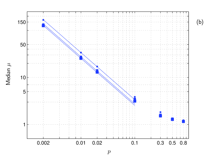
With the random initial condition, the quartiles of are very close to those obtained with the uniform initial condition.
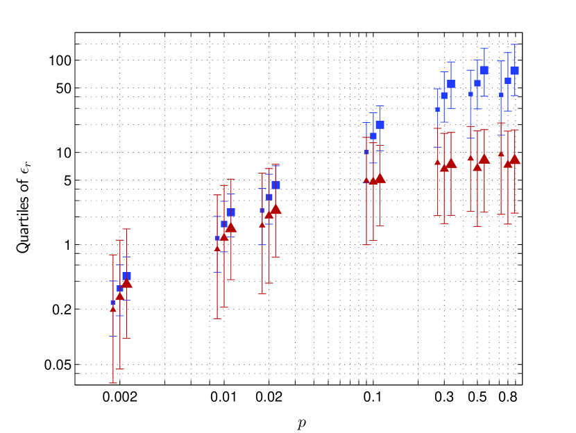
We then calculated for each basin the relative error between the mean sojourn time obtained from the uniform initial condition and that obtained from the random initial condition. This error is null at (as for the network of Fig. 1, this is because is geometric at ). The quartiles of the error tend to as and they reach a maximum at whatever the network ensemble. Thus the smaller , the more is independent of initial conditions.
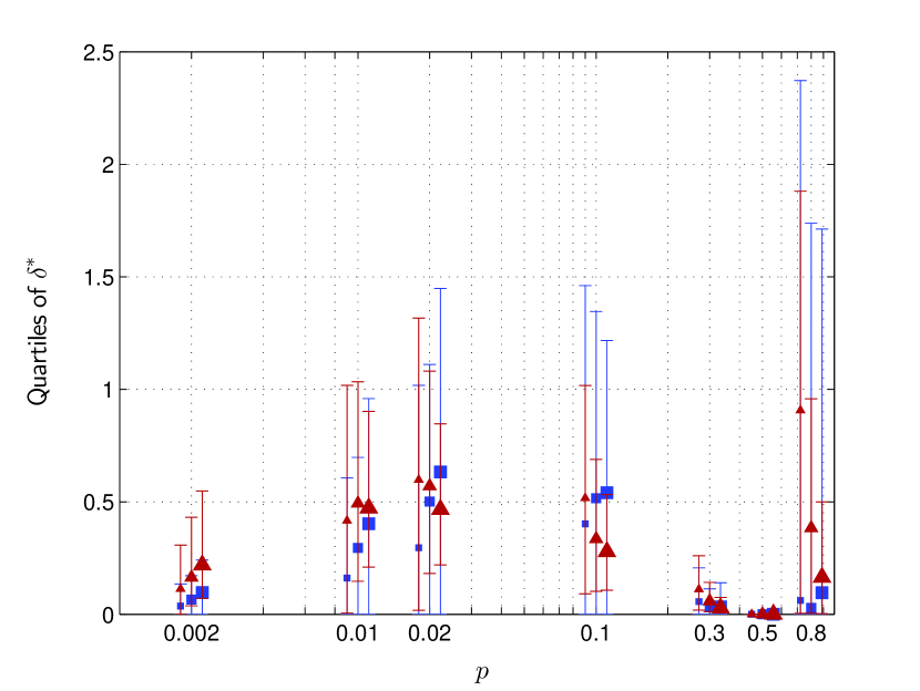
To end, we turn to the maximum deviation . First the uniform initial condition. The results for the six ensembles are presented in Fig. 11. At and for fixed , the quartiles increase linearly with , except the first quartile of basins which is constant and approximately equal to (whatever , of basins have a sojourn time that is geometric or closely follows a geometric distribution).
For both connectivities, the functions and have similarities with the functions of Fig. 4: they tend to when , they have at least one local maximum in and are null at .
With the random initial condition, the second and third quartiles of increase for most of the six ensembles compared to the uniform case. Qualitatively, the behaviour of the quartiles with respect to is similar to the one found with the uniform initial condition.
To summarize sections 3 and 4, we have the following proposition:
Proposition 3
Consider a basin of a noisy Boolean network. As tends to then:
-
1.
whatever the initial conditions, .
-
2.
tends to be independent of the initial conditions: with the Perron-Frobenius eigenvalue of fundamental matrix .
-
3.
whatever the initial conditions, , where is the Kolmogorov distance between the cumulative distribution function of the sojourn time in the basin and that of a geometric distribution having the same mean as .
-
4.
converges to an exponential distribution.
Proposition 3 does not guarantee the existence of a coarser representation of a NBN in the low regime. What can be said from this proposition is that if such a representation exists, then it is in general an approximation of the original process and it can always be expressed in a discrete or continuous time framework. Thus we are lead to the proposition below that will be discussed in more details in the next section:
Proposition 4
Consider a noisy Boolean network and suppose there exists a coarser time-homogeneous representation of this network in the low regime. Then the dynamics between the basins of the network may be approximated by a system of linear ordinary differential equations with size being equal to the number of attractors of the network.
Recall that Proposition 3 does not mean that can never be geometric nor be approximated by a geometric distribution when is not sufficiently close to . For example we know is geometric when or when whatever . One difference between a strongly and a weakly perturbed network is that in the latter, since the mean specific path is large compared to , the network spends long periods on the attractors without being perturbed. Under normal conditions, biochemical networks are supposed to work in the low regime because as explained in 1.2, this regime is associated with functional stability.
4.3 Approximation formula for the mean time spent in a basin of a NBN
For sufficiently small , th element of can be approximated by ():
From (24) then we may write:
| (28) |
We see that in the low regime, the probability depends on time and initial conditions.
Now for sufficiently small , we have the following:
| (29) |
which, from Proposition 2, is equivalent to:
To show approximation formula (29), we consider two cases:
-
1.
Suppose for any given , the elements of vector are equal. Then from (24) is constant which means geometric. Thus taking sufficiently small, must be the same for all state and therefore from (28):
(30) with and the size of the attractor.
Note that: (1) if , it comes that and therefore . (2) If , then is geometric since in this case is a symmetric matrix of size . If one starts with probability in one of the two states, then each probability will be periodic with period . (3) If is geometric then the parameter of the distribution may be written:
with and conditional probabilities defined as except that rather than perturbing one bit we perturb bits simultaneously. Taking sufficiently small in this formula, we retrieve approximation (30).
-
2.
If is not geometric, then for sufficiently small it comes from (28) that must tend to as since must tend to a value which is close to and to a value which is close to . From Propositions 1 and 2 then, we get (29) with:
Remark 6
| (31) |
Therefore, in the low regime, the mean time spent in a basin of a NBN is approximately proportional to the mean specific path . As shown in Fig. 12 for the six ensembles (ln-ln plot), the relative error done in approximation (31) decreases as becomes smaller. It can also be seen in the figure that in the low regime, being fixed, median increases with , and that while at fixed the median error for chaotic basins is smaller than for complex ones, the interquartile range for the former is greater than for the latter.
The statistical basin variables in equation (29) are and . Since the hyperbolic function is strictly monotone decreasing, the median of is equal to the inverse of the median of . Thus the constant in equation (27) must be approximately equal to , where stands for the median of . For , the values of were found to be (, and ) , and ; for , we found , and respectively. These values of are indeed very close to the values of that have been obtained by the least squares method in subsection 4.2 (the relative error between and ranges from to ).
The first and third quartiles of satisfy a relation of the same type as (27):
where and . The first (resp. third) quartile of is thus linked to the third (resp. first) quartile of . For each ensemble , we can define as many constants as there are percentiles.
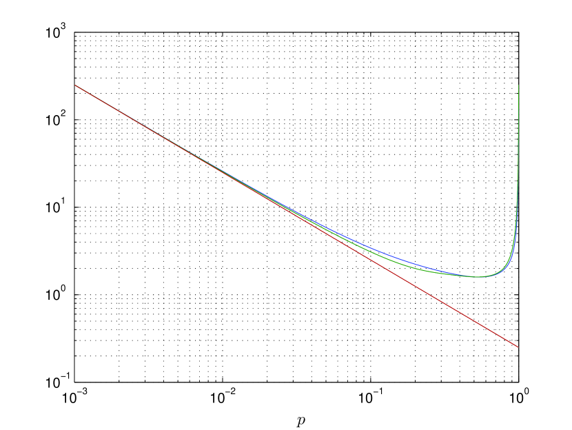
Fig. 13 shows (in blue), (in green) and (in red) versus (ln-ln plot) for basin B1 of Fig. 1 and the uniform initial condition. For small ( on the figure), these three functions behave identically. For , we see that . For basin B2 of Fig. 1 and the uniform initial condition, is very close to whatever (figure not shown). Thus formula may be accurate even if is not small, which is not the case for approximation .
Since , from (7) and (29) we can express through some approximation formulas valid in the low regime:
| (32) |
Since for sufficiently small , , we may write:
| (33) |
If is in the th main probability level (see 4.1), then:
| (34) |
If is geometric, then its parameter is equal to . Only in this case is the probability of leaving the basin during one time step equal to the inverse of the mean sojourn time . If is close to a geometric distribution (for some or all ), then is approximately constant, i.e. .
Let us mention another property. Let . Then
Equivalently, at fixed , the mean probability of leaving a basin calculated over a period of the attractor tends to be constant as time increases. The convergence is much more rapid than the one of (see Proposition 1).
Finally, we shall establish the general expression of the mean sojourn time when . The number of ways any state of an -node NBN can be perturbed is:
| (35) |
where the last equality follows from the Binomial Theorem. This means that whatever the perturbed state, any of the other states is reachable from that state by applying the appropriate perturbation combination out of the possible perturbation combinations (the chain is irreducible). Hence:
with, as before, the size of basin B. For , we know that is geometric, i.e. the probability does not depend on nor on the initial conditions. Thus:
| (36) | |||||
and thus
| (37) |
The bigger the basin, the smaller , the higher . The Perron-Frobenius eigenvalue of is and that of is . When we get . Notice that, since formula (37) depends only on and , it is also valid when .
Another way to get (36) is to notice that when , each element of (and ) is equal to . This means that
Since does not depend on time nor on initial state , must be geometric.
5 Method for the reduction of a NBN
5.1 Discrete-time reduction
5.1.1 The low regime
Consider an -basin NBN with state space size and Markov representation and suppose that the network has no basin. We want to find a discrete-time homogeneous Markov chain with state of the chain representing basin of the network, i.e. the state space of is . In the theory of Markov processes, would be called a reduced chain or aggregated chain because . The problem of reducing a Markov chain to a chain with a smaller state space, the so-called “state space explosion problem”, is not new (Kemeny and Snell,, 1960; Fredkin and Rice,, 1986) and is still an active field of research in the theory of Markov processes (Guédon et al.,, 2006; Grone et al.,, 2008; Weinan et al.,, 2008; Zhao et al.,, 2009). Here, we do not need to aggregate . The aggregation is fixed by the interactions that occur between the components of the network.
The expressions for the transition probabilities between the basins of the network are found as follows. For convenience, the validity of these formulas are discussed further below. From (32), we write:
where denotes the probability of basin (, ). Thus we have:
| (38) |
Probability can be expressed as a sum of probabilites:
| (39) |
with the conditional probability for a transition between basins and to occur given that one bit of attractor has been perturbed (). If (), then transition probability is taken to be:
| (40) |
Therefore in the low regime, is the product of two probabilities: the probability that one node be perturbed during one time step, which is approximately equal to for small , and the conditional probability .
Now if , one may transition to basin by perturbing at least two bits of an attractor state or at least one bit of a transient state. Since in the low regime the network is rarely found in transient states and for , when , transitions are rare events compared to transitions for which . Therefore we take .
By supposing that the time spent in any basin B of a NBN is geometric with mean , we neglect transitions of order from transient states as well as transitions of order or more (transitions from transient or attractor states due to perturbations affecting two or more nodes simultaneously). This means that while the original chain is irreducible, the reduced chain may not be irreducible anymore. If this is the case, the reduction method may give inaccurate results. Suppose that reduction of a NBN gives two sets of basins, each containing two basins that communicate with each other (each basin is accessible from the other), and that those sets are closed (by perturbing any node of any attractor state of any set, the other set cannot be reached). In Markov theory, such sets are called closed communicating classes. If we start in one set with probability one, then the state probability in the other set calculated from the reduced matrix will be at any time. Now if we solve the original chain, this will not be the case. If the stationary probability for the initially empty set is not negligible, then it will take a long time to approach this probability with good accuracy but it will. Another difference between these two chains is that the reduced one has an infinity of stationary distributions while the original one a unique stationary distribution.
If, starting in any basin, one can reach any other basin by applying single node perturbations to attractor states, then the reduced chain is irreducible. In this case, the smaller , the more accurate the reduction method. If the reduced chain is not irreducible, the reduction method is not guaranteed to work properly.
Remark 7
We investigated the case of reducible chains. Let be the probability distribution of the time spent in basin given and arrival basin . When , the first moment of may strongly depend on . We found some cases (some basins with some ) in the low regime for which was significantly smaller than .
To illustrate the chain reduction method, we chose a randomly generated network having basins of size , , and . The size of the corresponding attractors were , , and . We considered two values, namely and . The reduced matrix when was found to be:
| (41) |
This matrix is irreducible, i.e. any basin is accessible from any other basin by applying single-node perturbations to attractor states131313Notice that there is no basin ( ). If was null for some , we would have everywhere in row of except at position where we would have . Thus the reduced chain would be absorbing.. Also note that the second basin, which is the biggest one ( states), is the only state of which is reachable from any other state.
The four basin occupation probabilities versus time are shown in Fig. 14. The probabilities calculated from the matrix of the original chain , which we denote by , are represented in blue. At time , the network was put in state (state ) which is in B1, so that . The state probabilities of the reduced chain , calculated from the matrix , are shown in green. It is seen in Fig. 14a that for approximation is not good, in particular for basin B4. Results for are presented in Fig. 14b where it can be seen that the blue and green stairstep plots are almost identical, i.e. for , is a faithful coarse-grained representation of the NBN.
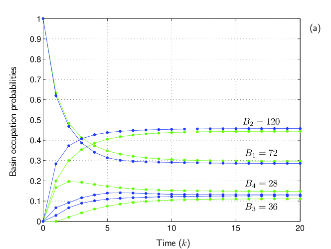
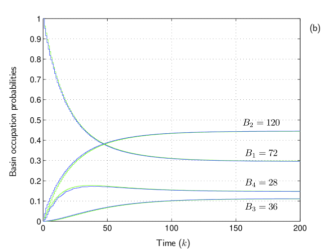
Also compared the stationary probabilities calculated from and (see 1.4). For , we found (basins , , and ) , , and when ;, , and when . For , the stationary probabilites are independent of (see below) and equal to , and . The maximum of the relative error is when and when . Thus in the long run, the most populated basin is the one with the greatest size () and the smaller probability ().
More generally, if chain is irreducible and aperiodic then its stationary state probability vector satisfies:
| (42) |
Rearranging the first equation in (42) we find:
where
| (43) |
From (39), matrix is singular. The stationary state probability vector of is thus an eigenvector of and the corresponding eigenvalue is .
In addition, the stationary state probability vector can be obtained by calculating the limit
| (44) |
where each row of the limit matrix is equal to the transposed stationary state probability vector.
5.1.2 Case
When , the reduction is “exact”. From (36), the probability to leave a basin of size is . The probability to remain in such a basin is thus . Since is geometric, one has:
| (45) |
with
and otherwise. Hence:
| (46) |
The rows of are thus equal. In fact, when , the stationary state is reached in one step whatever the initial conditions so that each row of gives the stationary state probabilities for the basins of the network. Note that since as , these stationary state probabilities can be used to approximate the stationary state probabilities in a neighborhood of .
From , the mean sojourn time in basin is expressed as:
5.2 Continuous-time reduction
The preceding sections deal with discrete-time homogeneous Markov chains. For such chains, the sojourn time spent in any state is geometric and thus memoryless. The continuous analog of the geometric distribution is the exponential distribution, which is also memoryless. Making the passage from geometric to exponential distribution leads to continuous-time homogeneous Markov chains. As we shall discuss, in the continuous-time representation of Markov processes, the state probabilities satisfy a system of linear ordinary differential equations.
A continuous-time Markov chain is homogeneous if the transition probability from state to state in time interval depends only on the length of the interval: . In this case (Kleinrock,, 1975):
| (47) |
with the rate of transition from state to state and
| (48) |
The time spent in state is exponentially distributed with parameter .
Now if is viewed as the continuous-time coarse-grained representation of an -basin NBN, then the state probabilities of satisfy the following Master equation (Kleinrock,, 1975):
| (49) |
As stated in Proposition 3, to allow the passage from discrete to continuous representation, only one needs to be sufficiently small. In other words, for sufficiently small , one may use instead of . A small implies that the mean specific path is large compared to . Since , a small also implies that is large compared to . As an example, compare Figs. 14a and 14b. In the first case, and whatever the basin, while in the second case, and is between and depending on the basin.
Example 4
Let us illustrate the passage from discrete-time chain to continuous-time reduced chain with the state diagram of Fig. 1. The reduced chain in this example has only two states so that from (48) we get: and . The equations for the reduced chain are thus:
Figs. 15a and 15b show B1 occupation probability versus time when and respectively. The blue points represent the solutions of equation (8) when initially the states of B1 are equiprobable and B2 is empty (for the sake of clarity, the points were interpolated linearly) while the green continuous curves are the solutions of system (4) when and . For (), the probability calculated from decreases by small amounts and seems to vary continuously with time (see the enlarged portion in Fig. 15b) so that continuous-time chain may be used instead of . Thus for sufficiently small , system of differential equations (4) may be used as a coarse-grained representation of the NBN.
To end this example, let us estimate the relative error between the inverse of the mean sojourn time and its approximation . The mean sojourn time for both basins and both values are given in Table 2. For one finds and , to be compared to and , which gives relative errors of and . For one gets and , to be compared to and , which gives relative errors of and .
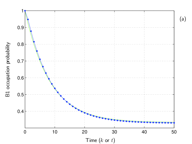
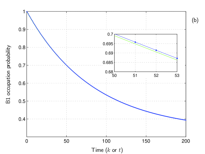
6 Statistical fluctuations in NBNs
Consider replicas of a given BN, i.e. cells expressing the same biochemical network, and suppose that each node of each replica may be perturbed with probability independently of time, of the other nodes and of the other replicas141414Statistical independence between the replicas means that whether at time a replica has been perturbed or not does not depend on whether between and other replicas have been perturbed or not..
The Markov chain model is a probabilistic model. Knowing the current state of a replica, this model allows to compute the probability of finding the replica in any given state of the network at any subsequent time. Therefore, even if the initial state of the replica is known with certainty, its trajectory in the state space of the network cannot be predicted with certainty. The same applies to the prediction of the number of replicas in each state of the network at any time.
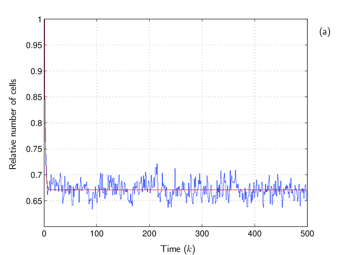
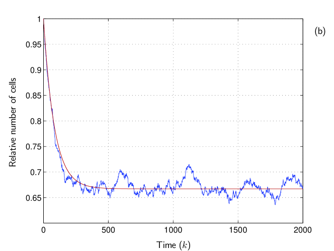
In order to illustrate the random behaviour of an ensemble of replicas, random trajectories were simulated in the state space of the network of Fig. 1 by the Monte Carlo method. At time , replicas were put in state then the number of replicas in each basin of the network at discrete times computed. The relative number of replicas in B2 versus time is shown in Fig. 16 for and two values of . Graph (a) corresponds to while graph (b) to . Each blue stairstep plot results from Monte Carlo simulations (one simulation is one trajectory of one replica), while each red one represents the mean solution calculated from (8). As can be seen from the two graphs, the uncertainty on the long-term behaviour of the ensemble is quite low in both cases (coefficient of variation: when and when ).
Remark 8
It is assumed that the total number of cells is conserved (cells do not proliferate and they are not lost):
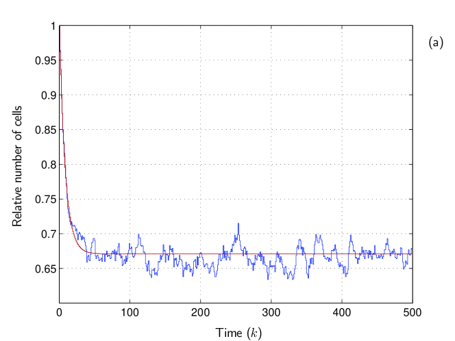
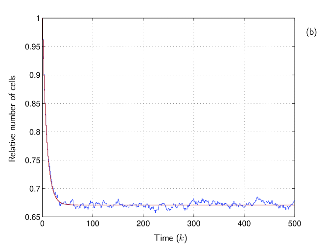
Also calculated was the probability distribution of the time spent in basin B2. The relative frequencies obtained from the Monte Carlo method are shown in blue in Fig. 17 for and cases. The red points represent the exact frequencies calculated from matrix as explained in section 2 (Markov method). For the sake of clarity, frequencies were interpolated linearly. Suppose that each Monte Carlo distribution in Fig. 17 results from the measurement of individual sojourn times. What would be the uncertainty on the mean time spent in B2 for each ensemble of cells ? The confidence interval would be with the case and with the one. The exact mean sojourn time is (Markov method, see Table 2).
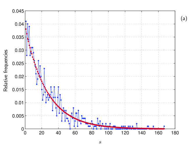
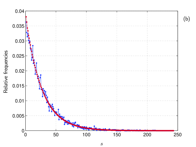
When is fixed and increases, the amplitude of the fluctuations in decreases as more and more replicas have a short sojourn time. By comparison of the graph of Fig. 16a and the two graphs of Fig. 18, the amplitude of the fluctuations in the relative number of replicas is not very sensitive to 151515Neither is the long-term B2 occupation probability: , and when , and respectively.. There is, however, a striking difference between Fig. 18a and Fig. 18b. When is small, the relative number of replicas in B2 remains above or below its stationary value for long periods, i.e. the width of the fluctuations increases when decreases. This means that in the low regime, the long-term behaviour of the network is characterized by slow transitions between two states: one that corresponds to an “overpopulated” attractor and the other to an “underpopulated” one. The probability of crossing the stationary value during one time step was found to be when and when ( when ). The maximum number of time steps the attractor remains overpopulated was when and when ( when ). Similar values were found for the underpopulated case.
Remark 9
(1) Since the number of replicas is conserved, when an attractor is overpopulated, the other is underpopulated and vice versa. (2) These slow transitions occuring in the low regime cannot be deduced from the Markov chain model.
7 Reduction of a NBN to a two-state Markov chain
We addressed the problem of reducing a chain to a two-state homogeneous chain by aggregating basins of attraction.
Only networks with were studied. The aggregation process consisted in the following. When was pair, basins were picked at random and aggregated, while when was odd basins were aggregated randomly. In both cases the remaining basins were aggregated, constituting the second state of the two-state chain. For each aggregated state then, we calculated the mean sojourn time with both types of initial conditions (the uniform and the random type) as well as the maximum deviation . Results indicate that as , does not tend to be independent of initial conditions neither does tend to . Notice, however, that the reduction of worked well in some cases (some networks with some basin aggregations).
8 Conclusion
The reduction method for NBNs presented in this paper raises the important question whether biochemical networks can be reduced to (approximating) coarse-grained networks functionally equivalent to the original ones. Reducing the complexity of biochemical networks could help in the analysis of cell responses to inputs (or cell fates) by neglecting molecular interactions while focusing on the higher-level processes that emerge from those interactions. A formally equivalent and very useful reduction theorem exists in electrical circuit theory which is Thevenin’s theorem.
9 Note
This work is part of a manuscript entitled “Mathematical modeling of cellular processes: from molecular networks to epithelial structures” written by F. Fourré. The complete manuscript contains five chapters. The first chapter is devoted to NBNs. The aim of the project is to propose a physical framework for describing cellular processes. Since 1st December 2008, F. Fourré has been working on a PhD thesis that is funded by the University of Luxembourg and supervised by Prof. Thomas Sauter. The thesis deals with qualitative modeling of signaling networks.
D. Baurain is a Postdoctoral Researcher of the FNRS.
10 Acknowledgment
F. Fourré gratefully thanks Prof. T. Sauter for having encourage him to write this paper and for the position of Assistant/PhD student at the Systems Biology Group of the University of Luxembourg.
References
- Dobson, (2003) Dobson, C. M. (2003). Protein folding and misfolding. Nature, 426:884–890.
- Douglas and Brian, (1999) Douglas, L. and Brian, M. (1999). An introduction to symbolic dynamics and coding. Cambridge University Press, New York.
- Fredkin and Rice, (1986) Fredkin, D. R. and Rice, J. A. (1986). On aggregated Markov processes. Journal of Applied Probability, 23:208–214.
- Glass and Kauffman, (1973) Glass, L. and Kauffman, S. A. (1973). The logical analysis of continuous non-linear biochemical control networks. J Theor Biol., 39:103–129.
- Grone et al., (2008) Grone, R., Hoffmann, K. H., and Salamon, P. (2008). An interlacing theorem for reversible Markov chains. J. Phys. A: Math. Theor., 41:212002.
- Guédon et al., (2006) Guédon, Y., d’Aubenton Carafa, Y., and Thermes, C. (2006). Analysing grouping of nucleotides in DNA sequences using lumped processes constructed from Markov chains. J Math Biol., 52:343–372.
- Kauffman, (1969) Kauffman, S. A. (1969). Metabolic stability and epigenesis in randomly connected nets. J Theor Biol., 22:437–467.
- Kauffman, (1993) Kauffman, S. A. (1993). The Origins of Order: Self-Organization and Selection in Evolution. Oxford University Press, New York.
- Kemeny and Snell, (1960) Kemeny, J. G. and Snell, J. L. (1960). Finite Markov Chains. D. Van Nostrand, London.
- Kleinrock, (1975) Kleinrock, L. (1975). Queueing Systems. Volume 1: Theory. John Wiley & Sons, New York.
- Li et al., (2004) Li, F., Long, T., Lu, Y., Ouyang, Q., and Tang, C. (2004). The yeast cell-cycle network is robustly designed. Proc Natl Acad Sci U S A, 101:4781–4786.
- Martin et al., (2007) Martin, S., Zhang, Z., Martino, A., and Faulon, J. L. (2007). Boolean dynamics of genetic regulatory networks inferred from microarray time series data. Bioinformatics, 23:866–874.
- Samal and Jain, (2008) Samal, A. and Jain, S. (2008). The regulatory network of E. coli metabolism as a Boolean dynamical system exhibits both homeostasis and flexibility of response. BMC Syst Biol., 2: 21.
- Shmulevich et al., (2002) Shmulevich, I., Dougherty, E. R., and Zhang, W. (2002). Gene perturbation and intervention in probabilistic Boolean networks. Bioinformatics, 18:1319–1331.
- Snell, (1959) Snell, J. L. (1959). Finite Markov chains and their applications. American Mathematical Monthly, 66:99–104.
- Weinan et al., (2008) Weinan, E., Li, T., and Vanden-Eijnden, E. (2008). Optimal partition and effective dynamics of complex networks. Proc Natl Acad Sci U S A, 105:7907–7912.
- Zhao et al., (2009) Zhao, Z., Weber, S., and de Oliveira, J. C. (2009). Preemption rates for a parallel link loss network. Performance Evaluation, 66:21–46.