TUW-09-21
UWThPh-2009-15 Loop Calculations for the Non-Commutative $U_{\star}(1)$ Gauge Field Model with Oscillator Term

Abstract

Motivated by the success of the non-commutative scalar Grosse-Wulkenhaar model, a non-commutative $U_{\star}(1)$ gauge field theory including an oscillator-like term in the action has been put forward in Blaschke:2007b . The aim of the current work is to analyze whether that action can lead to a fully renormalizable gauge model on non-commutative Euclidean space. In a first step, explicit one-loop graph computations are hence presented, and their results as well as necessary modifications of the action are successively discussed.

1 Introduction

One of the big challenges of the past decade has been the construction of renormalizable quantum field theories (QFTs) on non-commutative space-time, usually plagued by the infamous UV/IR mixing problem Minwalla:1999 , Douglas:2001 , Rivasseau:2007a . Only in very special cases has this task been successful so far, namely in the case of scalar field theories formulated in even dimensional $\theta$-deformed Euclidean space: In fact, three such renormalizable models are known today, the first of which being the so-called Grosse-Wulkenhaar model Grosse:2003 , Grosse:2004b , Rivasseau:2005a . In that model, the action is supplemented by an oscillator-like term which modifies the propagator in such a way that it becomes Langmann-Szabo invariant Szabo:2002 (just like the modified action, in fact).

Motivated by the success of the Grosse-Wulkenhaar model, some non-commutative gauge field models including similar oscillator-like terms in the action were put forward in Refs. Blaschke:2007b , Grosse:2007 , Wulkenhaar:2007 . The current work mainly deals with loop calculations based on the previous letter Blaschke:2007b , aiming to clarify whether the action we proposed there can lead to a renormalizable non-commutative gauge theory. In doing so, we find effective one-loop contributions to the action showing great similarities to the so-called “induced gauge theories” with oscillator terms which were put forward in Grosse:2007 , Wulkenhaar:2007 . These findings lead us to the conclusion, that (even though we do not claim to have solved the many problems concerning non-commutative gauge field theories in general, as was discussed in Blaschke:2009c ) the implementation of a Grosse-Wulkenhaar oscillator term into gauge theories seems to be a promising ansatz for a renormalizable non-commutative gauge theory. However, it also seems to be necessary to do this in a gauge invariant manner, i.e. to consider an action derived by (or motivated from) the “induced gauge theories”.

Our paper is organized as follows: Section 2 briefly reviews the action and its symmetries followed by Section 3 where some one-loop results are presented. We finally compare the effective action with the induced gauge theory of Grosse:2007 , Wulkenhaar:2007 in Section 4 and discuss the consequences.

2 The non-commutative gauge field model with oscillator term

In the simplest case of $\theta$-deformed space-time, one considers a constant commutator $\left[x^{\mu}\stackrel{{\scriptstyle\star}}{{,}}x^{\nu}\right]\equiv x^{\mu}\star x^{\nu}-x^{\nu}\star x^{\mu}={\rm i}\theta^{\mu\nu}$, i.e. a Heisenberg algebra for the space-time coordinates, realized through the so-called Groenewold-Moyal $\star$-product Groenewold:1946 , Moyal:1949 . Considering four dimensional Euclidean space, in Ref. Blaschke:2007b we proposed the following non-commutative $U_{\star}(1)$ gauge field action at tree-level:

$$\Gamma^{(0)} =S_{\text{inv}}+S_{\text{m}}+S_{\text{gf}}\,,$$

$$S_{\text{inv}} =\frac{1}{4}\int d^{4}x\,F_{\mu\nu}\star F_{\mu\nu}\,,$$

$$S_{\text{m}} =\frac{\Omega^{2}}{4}\int d^{4}x\left(\frac{1}{2}\left\{\tilde{x}_{\mu}\stackrel{{\scriptstyle\star}}{{,}}A_{\nu}\right\}\star\left\{\tilde{x}_{\mu}\stackrel{{\scriptstyle\star}}{{,}}A_{\nu}\right\}+\left\{\tilde{x}_{\mu}\stackrel{{\scriptstyle\star}}{{,}}\bar{c}\right\}\star\left\{\tilde{x}_{\mu}\stackrel{{\scriptstyle\star}}{{,}}c\right\}\right)=$$

$$=\frac{\Omega^{2}}{8}\int d^{4}x\left(\tilde{x}_{\mu}\star\mathcal{C}_{\mu}\right)\,,$$

$$S_{\text{gf}} =\int d^{4}x\Bigg{[}B\star\partial_{\mu}A_{\mu}-\frac{1}{2}B\star B-\bar{c}\star\partial_{\mu}sA_{\mu}-\frac{\Omega^{2}}{8}\,\widetilde{c}_{\mu}\star s\,\mathcal{C}_{\mu}\Bigg{]}\,,$$ (1)

with

$$F_{\mu\nu} =\partial_{\mu}A_{\nu}-\partial_{\nu}A_{\mu}-{\rm i}g\left[A_{\mu}\stackrel{{\scriptstyle\star}}{{,}}A_{\nu}\right]\,,$$

$$\mathcal{C}_{\mu} =\Big{(}\left\{\left\{\tilde{x}_{\mu}\stackrel{{\scriptstyle\star}}{{,}}A_{\nu}\right\}\stackrel{{\scriptstyle\star}}{{,}}A_{\nu}\right\}+\left[\left\{\tilde{x}_{\mu}\stackrel{{\scriptstyle\star}}{{,}}\bar{c}\right\}\stackrel{{\scriptstyle\star}}{{,}}c\right]+\left[\bar{c}\stackrel{{\scriptstyle\star}}{{,}}\left\{\tilde{x}_{\mu}\stackrel{{\scriptstyle\star}}{{,}}c\right\}\right]\Big{)}\,,$$

$$\tilde{x}_{\mu} =\left(\theta^{-1}\right)_{\mu\nu}x_{\nu}\,.$$ (2)

The field $A_{\mu}$ denotes the non-commutative generalization of a $U(1)$ gauge field (hence the notation $U_{\star}(1)$ for the deformed algebra), and $B$ is the multiplier field implementing a non-linear gauge fixing

$$\frac{\delta\Gamma^{(0)}}{\delta B} =\partial_{\mu}A_{\mu}-B+\frac{\Omega^{2}}{8}\Big{(}\left[\left\{\tilde{x}_{\mu}\stackrel{{\scriptstyle\star}}{{,}}c\right\}\stackrel{{\scriptstyle\star}}{{,}}\widetilde{c}_{\mu}\right]-\left\{\tilde{x}_{\mu}\stackrel{{\scriptstyle\star}}{{,}}\left[\widetilde{c}_{\mu}\stackrel{{\scriptstyle\star}}{{,}}c\right]\right\}\Big{)}=0.$$ (3)

Furthermore, we have an additional multiplier field $\widetilde{c}_{\mu}$ imposing on-shell BRST invariance of the expression $\mathcal{C}_{\mu}$, $\Omega$ is a constant parameter and $c$, $\bar{c}$ are the ghost/antighost, respectively. The action (2) is invariant under the BRST transformations given by

$$sA_{\mu}=D_{\mu}c=\partial_{\mu}c-{\rm i}g\left[A_{\mu}\stackrel{{\scriptstyle\star}}{{,}}c\right], s\bar{c}=B,$$

$$sc={\rm i}g{c}\star{c}, sB=0,$$

$$s\widetilde{c}_{\mu}=\tilde{x}_{\mu}, s^{2}\varphi=0\ \forall\ \varphi\in\left\{A_{\mu},B,c,\bar{c},\widetilde{c}_{\mu}\right\}.$$ (4)

Using these transformations, the action can be written succinctly as

$$\Gamma^{(0)}=\int d^{4}x\left(\frac{1}{4}F_{\mu\nu}\star F_{\mu\nu}+s\left(\frac{\Omega^{2}}{8}\tilde{c}_{\mu}\star\mathcal{C}_{\mu}+\bar{c}\star\partial_{\mu}A_{\mu}-\frac{1}{2}\bar{c}\star B\right)\right)\,.$$ (5)

The properties of the appearing fields are summarized in Table 1, where $g_{\sharp}$ denotes the ghost number.

Table 1: Properties of the fields.

Field	$A_{\mu}$	$c$	$\bar{c}$	$\tilde{c}_{\mu}$	$B$
$g_{\sharp}$	0	1	-1	-1	0
Mass dim.	1	0	2	1	2
Statistics	b	f	f	f	b

By introducing external sources $\rho_{\mu}$ and $\sigma$ for the non-linear BRST transformations, one derives the Slavnov-Taylor identity

$$\text{S}(\Gamma_{\text{tot}})=\int d^{4}x\,\Bigg{(}\frac{\delta\Gamma_{\text{tot}}}{\delta\rho_{\mu}}\star\frac{\delta\Gamma_{\text{tot}}}{\delta A_{\mu}}+\frac{\delta\Gamma_{\text{tot}}}{\delta\sigma}\star\frac{\delta\Gamma_{\text{tot}}}{\delta c}+B\star\frac{\delta\Gamma_{\text{tot}}}{\delta\bar{c}}+\tilde{x}_{\mu}\star\frac{\delta\Gamma_{\text{tot}}}{\delta\tilde{c}_{\mu}}\Bigg{)}=0\,,$$ (6)

with

$$\Gamma_{\text{tot}} =\Gamma^{(0)}+\Gamma_{\text{ext}}\,,$$

$$\Gamma_{\text{ext}} =\int d^{4}x\left(\rho_{\mu}\star sA_{\mu}+\sigma\star sc\right)\,.$$ (7)

Equation (6) describes the symmetry content with respect to (2). When taking its functional derivative with respect to $A_{\rho}$ and $c$ and then setting all fields to zero one arrives at

$$\partial^{z}_{\mu}\frac{\delta^{2}\Gamma_{\text{tot}}}{\delta A_{\rho}(y)\delta A_{\mu}(z)}=\int d^{4}x\,\Bigg{(}\tilde{x}_{\mu}\frac{\delta^{3}\Gamma_{\text{tot}}}{\delta c(z)\delta A_{\rho}(y)\delta\tilde{c}_{\mu}(x)}\Bigg{)}\neq 0\,.$$ (8)

Usually one would expect to obtain the transversality condition for the one-particle irreducible (1PI) two-point graph. However, in this case the oscillator term breaks gauge invariance and hence transversality, as can bee seen from the equation above: Instead one has a Ward identity relating the 1PI two-point graph to a three-point graph involving the new field $\widetilde{c}_{\mu}$. Graphically we can express this relation as depicted in Figure 1.

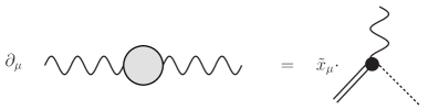
Figure 1: Ward identity replacing transversality

The bilinear parts of the action (2) lead to the following gauge field and ghost propagators in momentum space:

$$G^{A}_{\mu\nu}(p,q) =(2\pi)^{4}K_{M}(p,q)\delta_{\mu\nu},$$

$$G^{\bar{c}c}(p,q) =(2\pi)^{4}K_{M}(p,q)\,,$$ (9)

where $K_{M}(p,q)$ denotes the so-called Mehler kernel

$$K_{M}(p,q) =\frac{\omega^{3}}{8\pi^{2}}\int\limits_{0}^{\infty}d\alpha\frac{1}{\sinh^{2}(\alpha)}\exp\left(-\tfrac{\omega}{4}\coth\left(\tfrac{\alpha}{2}\right)\left(p-q\right)^{2}-\tfrac{\omega}{4}\tanh\left(\tfrac{\alpha}{2}\right)\left(p+q\right)^{2}\right),$$ (10)

which is going to be responsible for improving the IR behaviour of the model. In the limit $\omega=\frac{\theta}{\Omega}\to\infty$ these propagators reduce to the usual ones, i.e.

$$\lim\limits_{\Omega\to 0}K_{M}(p,q)=\frac{1}{p^{2}}\delta^{4}\left(p-q\right)\,.$$

This can be easily verified by integrating over one of the arguments in the Mehler kernel:

$$\lim\limits_{\Omega\to 0}\int d^{4}qK_{M}(p,q)=\lim\limits_{\Omega\to 0}\frac{1}{p^{2}}\left(1-{\rm e}^{-\frac{\omega}{2}p^{2}}\right)=\frac{1}{p^{2}}\,.$$ (11)

In the following sections we will discuss some one-loop properties of this model, but first some comments are in order: In contrast to the usual situation, the multiplier field $B$ appears in a $\widetilde{c}Bc$ vertex (in addition to the $BB$ and $BA$ propagators). However, since the new multiplier $\widetilde{c}_{\mu}$ does not propagate, it is impossible to build a graph including these additional Feynman rules, but with only external gauge field legs. In fact, these are the types of graphs we are going to concentrate on in the following, and hence the Feynman rules including the fields $B$ and $\widetilde{c}$ are ignored for now.

3 One-loop computations

3.1 Power counting

Before starting the explicit calculations, we may derive estimations for the “worst case”, i.e. the superficial degree of ultraviolet divergence, which via UV/IR mixing is directly related to the degree of non-commutative IR divergence. We take into account the powers of internal momenta $k$ each Feynman rule contributes and also that each loop integral over 4-dimensional space increases the degree by 4. For example, the gauge boson propagator usually behaves like $1/k^{2}$ for large $k$ and therefore reduces the degree of divergence by 2, whereas each ghost vertex contributes one power of $k$ to the numerator of a graph, hence increasing the degree by one. However, in the present model all propagators, being essentially Mehler kernels, depend on two momenta which additionally need to be integrated in loop calculations. Taking into account these considerations for all Feynman rules we arrive at

$$d_{\gamma}=4L-6I_{A}-6I_{c}-5I_{AB}-4I_{B}+V_{c}+V_{3A}+V_{\widetilde{c}cA}\,,$$ (12)

where the $I$ and $V$ denote the number of the various types of internal lines and vertices, respectively. The number of loop integrals $L$ is given by

$$L=2I_{A}+2I_{c}+2I_{B}+2I_{AB}-(V_{c}+V_{3A}+V_{4A}+V_{\widetilde{c}cA}+V_{\widetilde{c}c2A}+V_{\widetilde{c}Bc}+V_{\widetilde{c}\bar{c}2c}-1)\,.$$

Furthermore, we take into account the relations

$$E_{c/\bar{c}}+2I_{c} =2V_{c}+V_{\widetilde{c}cA}+V_{\widetilde{c}c2A}+V_{\widetilde{c}Bc}+3V_{\widetilde{c}\bar{c}2c}\,,$$

$$E_{A}+2I_{A}+I_{AB} =V_{c}+3V_{3A}+4V_{4A}+V_{\widetilde{c}cA}+2V_{\widetilde{c}c2A}\,,$$

$$E_{B}+2I_{B}+I_{AB} =V_{\widetilde{c}Bc}\,,$$

$$E_{\tilde{c}} =V_{\widetilde{c}cA}+V_{\widetilde{c}c2A}+V_{\widetilde{c}Bc}+V_{\widetilde{c}\bar{c}2c}\,,$$ (13)

between the various Feynman rules describing how they (and how many) can be connected to one another. The $E_{c/\bar{c}}$, $E_{A}$, $E_{\widetilde{c}}$ and $E_{B}$ denote the number of external lines of the respective fields. Using these relations one can eliminate all internal lines and vertices from the power counting formula and arrive at

$$d_{\gamma}=4-E_{A}-E_{c/\bar{c}}-E_{\tilde{c}}-2E_{B}\,.$$ (14)

For the gauge boson self-energy we therefore expect the degree of divergence (UV and non-commutative IR) to be at worst quadratically. Gauge invariance usually reduces the degree of UV divergence to be merely logarithmic. However, due to the Ward identity (8) whose right hand side is non-zero, the UV divergence will in fact be worse in our case, namely quadratic.

3.2 Tadpole graphs

The two possible one-point functions (tadpoles) of this model at one-loop level are depicted in Figure 2.

Figure 2: tadpole graphs

According to the Feynman rules given in (10) and in Appendix A, the sum of tadpole graphs is given by

$$\Pi_{\mu}(p) =2{\rm i}g\int d^{4}k\int d^{4}k^{\prime}\delta^{4}\left(p+k^{\prime}-k\right)\sin\left(\frac{k\tilde{p}}{2}\right)K_{M}(k,k^{\prime})\left[2k_{\mu}+3k^{\prime}_{\mu}\right]\,,$$ (15)

where the abbreviation $\tilde{p}_{\mu}\equiv\theta_{\mu\nu}p_{\nu}$ has been introduced. In the following, we furthermore assume that the deformation matrix $(\theta_{\mu\nu})$ has the simple block-diagonal form

$$(\theta_{\mu\nu})=\theta\left(\begin{array}[]{cccc}0&1&0&0\\ -1&0&0&0\\ 0&0&0&1\\ 0&0&-1&0\end{array}\right)\,,\qquad{\rm with}\ \;\theta\in\mathbb{R}\,.$$ (20)

Hence one has the identity $\tilde{p}^{2}=\theta^{2}p^{2}$ which will significantly simplify calculations. Making use of

$$\sin\left(\frac{k\tilde{p}}{2}\right)=\sum_{\eta=\pm 1}\frac{\eta}{2{\rm i}}\exp\left(\frac{{\rm i}\eta}{2}k\tilde{p}\right)\,,$$ (21)

and considering “short” and “long” variables defined by $u=k-k^{\prime}$ and $v=k+k^{\prime}$ one arrives at

$$\Pi^{\varepsilon}_{\mu}(p) =\frac{g\omega^{3}}{2^{8}\pi^{2}}\sum\limits_{\eta=\pm 1}\int d^{4}v\left[5v_{\mu}-p_{\mu}\right]\int\limits_{\varepsilon}^{\infty}d\alpha\frac{\eta{\rm e}^{\frac{{\rm i}\eta}{4}v\tilde{p}}}{\sinh^{2}\alpha}\exp\left(-\tfrac{\omega}{4}\left[\coth\left(\tfrac{\alpha}{2}\right)p^{2}+\tanh\left(\tfrac{\alpha}{2}\right)v^{2}\right]\right)$$

$$=\frac{5{\rm i}g\tilde{p}_{\mu}}{64}\int\limits_{\varepsilon}^{\infty}d\alpha\frac{\cosh\left(\frac{\alpha}{2}\right)}{\sinh^{5}\left(\frac{\alpha}{2}\right)}\exp\left[-\frac{1}{4}\coth\left(\frac{\alpha}{2}\right)\left(\omega+\frac{\theta^{2}}{4\omega}\right)p^{2}\right]\,,$$ (22)

regularizing the integrals by introducing a UV cutoff $\varepsilon=1/\Lambda^{2}$. Now we consider the following expansion:

$$\int\frac{d^{4}p}{(2\pi)^{4}}\,\Pi^{\varepsilon}_{\mu}(p) \left[A_{\mu}(0)+p_{\nu}\left(\partial^{p}_{\nu}A_{\mu}(p)\big{|}_{p=0}\right)+\frac{p_{\nu}p_{\rho}}{2}\left(\partial^{p}_{\nu}\partial^{p}_{\rho}A_{\mu}(p)\big{|}_{p=0}\right)+\right.$$

$$\left.\;+\frac{p_{\nu}p_{\rho}p_{\sigma}}{6}\left(\partial^{p}_{\nu}\partial^{p}_{\rho}\partial^{p}_{\sigma}A_{\mu}(p)\big{|}_{p=0}\right)+\ldots\right]\,.$$ (23)

All terms of even order (i.e. of order 0,2,4,…) are zero for symmetry reasons. Of the other terms, we now show that only the first two, namely orders 1 and 3, diverge in the limit $\varepsilon\to 0$:

• order 1:

  $$\int\frac{d^{4}p}{(2\pi)^{4}}\,p_{\nu}\Pi^{\varepsilon}_{\mu}(p) =\int\limits_{\varepsilon}^{\infty}d\alpha\frac{5{\rm i}g\theta_{\mu\nu}}{32\pi^{2}\omega^{3}\left(1+\frac{\Omega^{2}}{4}\right)^{3}\sinh^{2}(\alpha)}$$

  $$=\frac{5{\rm i}g\theta_{\mu\nu}}{32\pi^{2}\omega^{3}\left(1+\frac{\Omega^{2}}{4}\right)^{3}}\left[\frac{1}{\varepsilon}-1+\mathcal{O}(\varepsilon)\right].$$ (24)

  With the external field, we obtain a counter term of the form

  $$\left(\partial^{p}_{\nu}A_{\mu}(p)\big{|}_{p=0}\right) \int\frac{d^{4}p}{(2\pi)^{4}}\,p_{\nu}\Pi^{\varepsilon}_{\mu}(p)=$$

  $$=\frac{5g\Omega^{2}}{32\pi^{2}\omega\left(1+\frac{\Omega^{2}}{4}\right)^{3}}\left[\frac{1}{\varepsilon}-1+\mathcal{O}(\varepsilon)\right]\int d^{4}x\,\tilde{x}_{\mu}A_{\mu}(x)\,.$$ (25)

• order 3:

  $$\int\frac{d^{4}p}{(2\pi)^{4}}\,\frac{p_{\alpha}p_{\beta}p_{\gamma}}{6}\Pi^{\varepsilon}_{\mu}(p) =\frac{-5{\rm i}g\left(\delta_{\alpha\beta}\theta_{\mu\gamma}+\delta_{\beta\gamma}\theta_{\mu\alpha}+\delta_{\alpha\gamma}\theta_{\mu\beta}\right)}{24\pi^{2}\omega^{4}\left(1+\frac{\Omega^{2}}{4}\right)^{4}}\left[\ln\varepsilon+\mathcal{O}(0)\right],$$ (26)

  and with the external field we get the counter term

  $$\left(\partial^{p}_{\alpha}\partial^{p}_{\beta}\partial^{p}_{\gamma}A_{\mu}(p)\big{|}_{p=0}\right) \int\frac{d^{4}p}{(2\pi)^{4}}\,\frac{p_{\alpha}p_{\beta}p_{\gamma}}{6}\Pi^{\varepsilon}_{\mu}(p)=$$

  $$=\frac{5g}{8\pi^{2}}\frac{\Omega^{4}}{\left(1+\frac{\Omega^{2}}{4}\right)^{4}}\left[\ln\varepsilon+\mathcal{O}(0)\right]\int d^{4}x\,\tilde{x}_{\mu}{\tilde{x}}^{2}A_{\mu}(x)\,.$$ (27)

• order 5 and higher:
  These orders are finite. The contribution to order $5+2n$, $n\geq 0$ is proportional to

  $$\int\limits_{0}^{\infty}d\alpha\frac{\sinh^{n}\frac{\alpha}{2}}{\cosh^{n+4}\frac{\alpha}{2}}=\frac{4}{(n+1)(n+3)}\,.$$ (28)

Notice, that all tadpole contributions would vanish in the limit $\Omega\to 0$ as expected. When keeping $\Omega\neq 0$, the two divergent terms can be removed by renormalization, i.e. by considering the appropriate counter terms given in Eqns. (• ‣ 3.2) and (• ‣ 3.2), respectively. Remarkably, these terms are present in the induced action calculated in Refs. Grosse:2007 , Wulkenhaar:2007 . The fact that these graphs do not vanish also means that we need to find the correct vacuum for $\Omega\neq 0$ by solving the equations of motion, which at the classical level read

$$\frac{\delta\Gamma^{(0)}}{\delta A_{\nu}} =\left(-\Delta_{4}+\Omega^{2}\tilde{x}^{2}\right)A_{\nu}+{\rm i}g\left[A_{\mu}\stackrel{{\scriptstyle\star}}{{,}}F_{\mu\nu}\right]+{\rm i}g\partial_{\mu}\left[A_{\mu}\stackrel{{\scriptstyle\star}}{{,}}A_{\nu}\right]+{\rm i}g\left\{\partial_{\nu}\bar{c}\stackrel{{\scriptstyle\star}}{{,}}c\right\}+$$

$$\quad\;\,+\partial_{\nu}(\partial A)-\partial_{\nu}B+\frac{\Omega^{2}}{8}\Big{(}\left\{\left[D_{\nu}c\stackrel{{\scriptstyle\star}}{{,}}\widetilde{c}_{\mu}\right]\stackrel{{\scriptstyle\star}}{{,}}\tilde{x}_{\mu}\right\}+\left[\left\{D_{\nu}c\stackrel{{\scriptstyle\star}}{{,}}\tilde{x}_{\mu}\right\}\stackrel{{\scriptstyle\star}}{{,}}\widetilde{c}_{\mu}\right]\Big{)}-$$

$$\quad\;\,-{\rm i}g\frac{\Omega^{2}}{8}\Big{(}\left\{c\stackrel{{\scriptstyle\star}}{{,}}\left\{\tilde{x}_{\mu}\stackrel{{\scriptstyle\star}}{{,}}\left\{A_{\nu}\stackrel{{\scriptstyle\star}}{{,}}\widetilde{c}_{\mu}\right\}\right\}\right\}+\left\{c\stackrel{{\scriptstyle\star}}{{,}}\left\{\widetilde{c}_{\mu}\stackrel{{\scriptstyle\star}}{{,}}\left\{\tilde{x}_{\mu}\stackrel{{\scriptstyle\star}}{{,}}A_{\nu}\right\}\right\}\right\}\Big{)}=0,$$ (29a)

$$\frac{\delta\Gamma^{(0)}}{\delta B} =\partial_{\mu}A_{\mu}-B+\frac{\Omega^{2}}{8}\Big{(}\left[\left\{\tilde{x}_{\mu}\stackrel{{\scriptstyle\star}}{{,}}c\right\}\stackrel{{\scriptstyle\star}}{{,}}\widetilde{c}_{\mu}\right]-\left\{\tilde{x}_{\mu}\stackrel{{\scriptstyle\star}}{{,}}\left[\widetilde{c}_{\mu}\stackrel{{\scriptstyle\star}}{{,}}c\right]\right\}\Big{)}=0,$$ (29b)

$$\frac{\delta\Gamma^{(0)}}{\delta\bar{c}} =\left(-\Delta_{4}+\Omega^{2}\tilde{x}^{2}\right)c-{\rm i}g\frac{\Omega^{2}}{8}\Big{(}\left\{\left\{\tilde{x}_{\mu}\stackrel{{\scriptstyle\star}}{{,}}c\star c\right\}\stackrel{{\scriptstyle\star}}{{,}}\widetilde{c}_{\mu}\right\}+\left\{\tilde{x}_{\mu}\stackrel{{\scriptstyle\star}}{{,}}\left\{\widetilde{c}_{\mu}\stackrel{{\scriptstyle\star}}{{,}}c\star c\right\}\right\}\Big{)}$$

$$\quad+{\rm i}g\partial_{\mu}\left[A_{\mu}\stackrel{{\scriptstyle\star}}{{,}}c\right]=0,$$ (29c)

$$\frac{\delta\Gamma^{(0)}}{\delta c} =\left(\Delta_{4}-\Omega^{2}\tilde{x}^{2}\right)\bar{c}+\frac{\Omega^{2}}{8}\Big{(}\left\{\widetilde{c}_{\mu}\stackrel{{\scriptstyle\star}}{{,}}\left\{\tilde{x}_{\mu}\stackrel{{\scriptstyle\star}}{{,}}B\right\}\right\}+\left\{\tilde{x}_{\mu}\stackrel{{\scriptstyle\star}}{{,}}\left\{\widetilde{c}_{\mu}\stackrel{{\scriptstyle\star}}{{,}}B\right\}\right\}\Big{)}-$$

$$\quad\;\,-{\rm i}g\left[A_{\mu}\stackrel{{\scriptstyle\star}}{{,}}\partial_{\mu}\bar{c}\right]-\frac{\Omega^{2}}{8}D_{\nu}\Big{(}\left\{\tilde{x}_{\mu}\stackrel{{\scriptstyle\star}}{{,}}\left\{A_{\nu}\stackrel{{\scriptstyle\star}}{{,}}\widetilde{c}_{\mu}\right\}\right\}+\left\{\left\{\tilde{x}_{\mu}\stackrel{{\scriptstyle\star}}{{,}}A_{\nu}\right\}\stackrel{{\scriptstyle\star}}{{,}}\widetilde{c}_{\mu}\right\}\Big{)}+$$

$$\quad\;\,+{\rm i}g\frac{\Omega^{2}}{8}\Big{(}\left[c\stackrel{{\scriptstyle\star}}{{,}}\left[\widetilde{c}_{\mu}\stackrel{{\scriptstyle\star}}{{,}}\left\{\tilde{x}_{\mu}\stackrel{{\scriptstyle\star}}{{,}}\bar{c}\right\}\right]\right]-\left[c\stackrel{{\scriptstyle\star}}{{,}}\left\{\tilde{x}_{\mu}\stackrel{{\scriptstyle\star}}{{,}}\left[\bar{c}\stackrel{{\scriptstyle\star}}{{,}}\widetilde{c}_{\mu}\right]\right\}\right]\Big{)}=0,$$ (29d)

$$\frac{\delta\Gamma^{(0)}}{\delta\widetilde{c}_{\mu}} =-\frac{\Omega^{2}}{8}s\,\mathcal{C}_{\mu}=0.$$ (29e)

Finding solutions to these equations is the task of a work in progress.

3.3 Two point functions at one-loop level

In this section we analyze the divergence structure of the gauge boson self-energy at one-loop level. The relevant graphs are depicted in Figure 3.

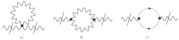
Figure 3: Gauge boson self-energy — amputated graphs

Explicitly, the sum of these graphs is computed using the same techniques as in the previous section (except for the expansion which is not necessary here). Once more we use long and short variables such as $u=k-k^{\prime}$ and $v=k+k^{\prime}$ and including their symmetry factors arrive at the following expressions for the three separate graphs:

$$\Pi^{a}_{\mu\nu} =-\frac{3g^{2}\delta_{\mu\nu}}{8}\int d^{4}v\,K_{M}(p-p^{\prime},v)\Big{[}\sin\left(\tfrac{(v+p^{\prime})\tilde{p}}{4}\right)\sin\left(\tfrac{(v+p)\tilde{p}^{\prime}}{4}\right)$$

$$\quad\hskip 150.79968pt+\sin\left(\tfrac{(v-p^{\prime})\tilde{p}}{4}\right)\sin\left(\tfrac{(v-p)\tilde{p}^{\prime}}{4}\right)\Big{]}\,,$$ (30a)

$$\Pi^{b}_{\mu\nu} =\frac{g^{2}}{8}\int d^{4}u\,d^{4}v\,K_{M}(u,v)K_{M}(u+p-p^{\prime},v+p+p^{\prime})\sin\left(\tfrac{(v+u)\tilde{p}}{4}\right)\sin\left(\tfrac{(v-u)\tilde{p}^{\prime}}{4}\right)$$

$$\quad\qquad\times\Big{[}\tfrac{5}{2}(v_{\mu}v_{\nu}-u_{\mu}u_{\nu})+\tfrac{3}{2}(u_{\mu}v_{\nu}-v_{\mu}u_{\nu})+\tfrac{1}{2}p^{\prime}_{\mu}(v+u)_{\nu}+\tfrac{1}{2}(v-u)_{\mu}p_{\nu}$$

$$\quad\qquad\qquad+2p_{\mu}(v-u)_{\mu}+2(v+u)_{\mu}p^{\prime}_{\nu}+2p_{\mu}p^{\prime}_{\nu}-4p^{\prime}_{\mu}p_{\nu}$$

$$\quad\qquad\qquad+\delta_{\mu\nu}\left(\tfrac{v^{2}-u^{2}}{2}+\tfrac{p^{\prime}(v+u)}{2}+\tfrac{(v-u)p}{2}+5pp^{\prime}\right)\Big{]}\,,$$ (30b)

$$\Pi^{c}_{\mu\nu} =\frac{-g^{2}}{16}\int d^{4}u\,d^{4}v\,K_{M}(u,v)K_{M}(u+p-p^{\prime},v+p+p^{\prime})\,(v+u)_{\mu}(v-u+2p^{\prime})_{\nu}$$

$$\quad\hskip 76.82234pt\times\sin\left(\tfrac{(v+u)\tilde{p}}{4}\right)\sin\left(\tfrac{(v-u)\tilde{p}^{\prime}}{4}\right)\,,$$ (30c)

where $p$ and $p^{\prime}$ denote the external momenta. In the limit $\Omega\to 0$ one would expect a result $\Pi_{\mu\nu}(p,p^{\prime})=\Pi_{\mu\nu}(p)\delta^{4}(p-p^{\prime})$ where the transversality property $p_{\mu}\Pi_{\mu\nu}=0$ holds. However, due to $\Omega\neq 0$ these properties are not fulfilled, i.e. transversality is broken and one cannot split off a delta function. In order to reveal the divergence structure of the general result without the “smeared out delta function”, we additionally integrate over $p^{\prime}$. Finally, noticing that the parameter integrals entering from the Mehler kernels (10), are dominated by the region of small $\alpha$, one also needs to approximate for $\alpha\ll 1$ in order to extract the UV and IR divergent terms. We hence arrive at

$$\Pi_{\mu\nu}^{\text{div}}(p) =\frac{g^{2}\delta_{\mu\nu}\left(1-\tfrac{3}{4}\Omega^{2}\right)}{4\pi^{2}\omega\,\varepsilon\left(1+\tfrac{\Omega^{2}}{4}\right)^{3}}+\frac{3g^{2}\delta_{\mu\nu}\Omega^{2}}{8\pi^{2}\tilde{p}^{2}\left(1+\tfrac{\Omega^{2}}{4}\right)^{2}}+\frac{2g^{2}\tilde{p}_{\mu}\tilde{p}_{\nu}}{\pi^{2}(\tilde{p}^{2})^{2}\left(1+\tfrac{\Omega^{2}}{4}\right)^{2}}$$

$$\quad+\text{logarithmic UV divergence}\,.$$ (31)

In the limit $\Omega\to 0$ (i.e. $\omega\to\infty$) this expression reduces to the usual transversal term

$$\lim\limits_{\Omega\to 0}\Pi_{\mu\nu}^{\text{div}}(p) =\frac{2g^{2}}{\pi^{2}}\frac{\tilde{p}_{\mu}\tilde{p}_{\nu}}{(\tilde{p}^{2})^{2}}+\text{logarithmic UV divergence}\,,$$ (32)

which is quadratically IR divergent in the external momentum $p$ and logarithmically UV divergent. Notice that the general result (3.3), on the other hand, not only breaks transversality due to the first two terms, but also has an ultraviolet divergence parameterized by $\varepsilon$, whose degree of divergence is higher compared to the (commutative) gauge model without oscillator term. Both properties are due to the term $S_{\text{m}}$ in the action which breaks gauge invariance (cf. Eqn. (8)).

3.4 Vertex corrections at one-loop level

The calculation of the vertex corrections generally proceeds along the lines of the previous section. Due to the vast amount of terms, it is however useful to use a computer: In fact we “taught” Wolfram Mathematica${}^{\text{\textregistered}}$ to perform exactly the same steps that we would have done by hand.

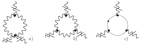
Figure 4: One loop corrections to the 3A-vertex.

Hence, computing the graphs depicted in Fig. 4 (and approximating for momentum conservation as in the previous subsections), one eventually finds a linear IR divergence of the form:

$$\Gamma^{\text{3A,IR}}_{\mu\nu\rho}(p_{1},p_{2},p_{3})=\frac{-8{\rm i}g^{3}}{\pi^{2}\left(4+\Omega^{2}\right)^{3}}\sum\limits_{i=1}^{3}\bigg{[} \frac{16\tilde{p}_{i,\mu}\tilde{p}_{i,\nu}\tilde{p}_{i,\rho}}{\tilde{p}_{i}^{4}}+\frac{3\Omega^{2}}{\tilde{p}_{i}^{2}}\left(\delta_{\mu\nu}\tilde{p}_{i,\rho}+\delta_{\mu\rho}\tilde{p}_{i,\nu}+\delta_{\nu\rho}\tilde{p}_{i,\mu}\right)\bigg{]},$$ (33)

where $p_{3}=-p_{1}-p_{2}$. Once more, this expression is not transversal due to the non-vanishing oscillator term parametrized by $\Omega$. However, in the limit $\Omega\to 0$ transverality is recovered, and (33) reduces to the well-known expression Matusis:2000jf , Armoni:2000xr , Ruiz:2000

$$\lim\limits_{\Omega\to 0}V^{\text{1loop}}_{\mu\nu\rho}(p_{1},p_{2},p_{3})=\frac{-2{\rm i}g^{3}}{\pi^{2}}\sum\limits_{i=1}^{3}\bigg{[} \frac{\tilde{p}_{i,\mu}\tilde{p}_{i,\nu}\tilde{p}_{i,\rho}}{\tilde{p}_{i}^{4}}\bigg{]}.$$ (34)

In the ultraviolet, the graphs of Fig. 4 diverge only logarithmically.

Additionally, one has of course also one-loop corrections to the 4A-vertex $\Gamma^{\text{4A,IR}}_{\mu\nu\rho\sigma}$. However, these show only a logarithmic divergence, as expected from the power counting (14).

4 Discussion

As already mentioned, the occurring UV counter terms of Section 3 are present in the induced gauge action, e.g. Grosse:2007 , Wulkenhaar:2007 . Let us compare the expressions in more detail here. The induced (Euclidean) gauge action (in the notation of Grosse:2007 ) is given by

$$\Gamma_{I}=\int d^{4}x\,\bigg{\{} \frac{3}{\theta_{I}}\left(1-\rho_{I}^{2}\right)\left(\tilde{\mu}_{I}^{2}-\rho_{I}^{2}\right)\left(\tilde{X}_{\nu}\star\tilde{X}_{\nu}-\tilde{x}^{2}\right)$$

$$+\frac{3}{2}\left(1-\rho_{I}^{2}\right)^{2}\left(\left(\tilde{X}_{\mu}\star\tilde{X}_{\mu}\right)^{\star 2}-\left(\tilde{x}^{2}\right)^{2}\right)+\frac{\rho_{I}^{4}}{4}F_{\mu\nu}\star F_{\mu\nu}\bigg{\}}\,,$$ (35)

where

$$\rho_{I}=\frac{1-\Omega_{I}^{2}}{1+\Omega_{I}^{2}},\qquad\tilde{\mu}_{I}^{2}=\frac{\mu_{I}^{2}\theta_{I}}{1+\Omega_{I}^{2}}\,.$$ (36)

The parameter $\mu_{I}$ denotes the mass of the scalar field. Through its coupling to $A_{\mu}$, the scalar field “induced” the effective one-loop action (4) above. The so-called covariant coordinates $\tilde{X}_{\mu}$ are furthermore defined as

$$\tilde{X}_{\mu} =\tilde{x}_{\mu}+A_{\mu}\,.$$ (37)

The first expression in the induced action (4) can be written as

$$\frac{3}{\theta_{I}}\left(1-\rho_{I}^{2}\right)\left(\tilde{\mu}_{I}^{2}-\rho_{I}^{2}\right)\left(\tilde{X}_{\nu}\star\tilde{X}_{\nu}-\tilde{x}^{2}\right)=\frac{3}{\theta_{I}}\left(1-\rho_{I}^{2}\right)\left(\tilde{\mu}_{I}^{2}-\rho_{I}^{2}\right)\left(2\tilde{x}_{\nu}A_{\nu}+A_{\nu}\star A_{\nu}\right)\,.$$ (38)

The first term of (38) has to be compared with the first expression in (• ‣ 3.2), whereas the second one corresponds to the first term of the self energy (3.3). However, the exact coefficients do not match. But since (• ‣ 3.2) and (3.3) only take one-loop effects into account this cannot be expected. Due to technical difficulties, we did not calculate the logarithmic UV divergences in all cases. Therefore, we can only compare the term proportional to $\tilde{x}^{2}(\tilde{x}A)$ given in Eq.(• ‣ 3.2). The respective term in the induced action — stemming from the $(\tilde{X}_{\mu}\star\tilde{X}_{\mu})^{2}$ term — reads

$$6\left(1-\rho_{I}^{2}\right)^{2}\tilde{x}^{2}\left(\tilde{x}A\right)\,.$$ (39)

In conclusion, one can state that the induced gauge theory action of Refs. Grosse:2007 , Wulkenhaar:2007 seems to be the more fundamental one when considering non-commutative gauge theories with Grosse-Wulkenhaar oscillator terms. The UV counter terms we have encountered here can be nicely accommodated. However, these models exhibit non-trivial vacuum configurations (which are discussed in e.g. Grosse:2007jy , Wallet:2008a , Wohlgenannt:2008mn ) due to non-vanishing tadpoles, and it is hence not (yet) clear, how to do higher order loop calculations. Especially, a (highly desirable) general proof of renormalizability will be very involved.

Acknowledgements

The authors are indebted to R. Sedmik for providing valuable assistance with Wolfram Mathematica${}^{\text{\textregistered}}$.
The work of D. N. Blaschke, E. Kronberger and M. Wohlgenannt was supported by the “Fonds zur Förderung der Wissenschaftlichen Forschung” (FWF) under contracts P20507-N16 and P21610-N16.

Appendix A Vertices

The vertices used for the graphs in Section 3 are given by

$$\widetilde{V}^{3A}_{\rho\sigma\tau}(k_{1},k_{2},k_{3}) =2{\rm i}g(2\pi)^{4}\delta^{4}(k_{1}+k_{2}+k_{3})\left[(k_{3}-k_{2})_{\rho}\delta_{\sigma\tau}\right.$$

$$\quad\quad\left.+(k_{1}-k_{3})_{\sigma}\delta_{\rho\tau}+(k_{2}-k_{1})_{\tau}\delta_{\rho\sigma}\right]\sin\left(\frac{k_{1}\tilde{k}_{2}}{2}\right),$$ (40a)

$$\widetilde{V}^{4A}_{\rho\sigma\tau\epsilon}(k_{1},k_{2},k_{3},k_{4}) =-4g^{2}(2\pi)^{4}\delta^{4}(k_{1}+k_{2}+k_{3}+k_{4})$$

$$\quad\times\left[(\delta_{\rho\tau}\delta_{\sigma\epsilon}-\delta_{\rho\epsilon}\delta_{\sigma\tau})\sin\left(\frac{k_{1}\tilde{k}_{2}}{2}\right)\sin\left(\frac{k_{3}\tilde{k}_{4}}{2}\right)\right.$$

$$\quad\quad\left.+(\delta_{\rho\sigma}\delta_{\tau\epsilon}-\delta_{\rho\epsilon}\delta_{\sigma\tau})\sin\left(\frac{k_{1}\tilde{k}_{3}}{2}\right)\sin\left(\frac{k_{2}\tilde{k}_{4}}{2}\right)\right.$$

$$\quad\quad\left.+(\delta_{\rho\sigma}\delta_{\tau\epsilon}-\delta_{\rho\tau}\delta_{\sigma\epsilon})\sin\left(\frac{k_{2}\tilde{k}_{3}}{2}\right)\sin\left(\frac{k_{1}\tilde{k}_{4}}{2}\right)\right],$$ (40b)

$$\widetilde{V}^{c}_{\mu}(q_{1},k_{2},q_{3}) =-2{\rm i}g(2\pi)^{4}\delta^{4}(q_{1}+k_{2}+q_{3})q_{3\mu}\sin\left(\frac{q_{1}\tilde{q}_{3}}{2}\right).$$ (40c)

References

• [1] D. N. Blaschke, H. Grosse and M. Schweda, Non-Commutative U(1) Gauge Theory on $\mathbb{R}^{4}$ with Oscillator Term and BRST Symmetry, Europhys. Lett. 79 (2007) 61002, [arXiv:0705.4205].
• [2] S. Minwalla, M. Van Raamsdonk and N. Seiberg, Noncommutative perturbative dynamics, JHEP 02 (2000) 020, [arXiv:hep-th/9912072].
• [3] M. R. Douglas and N. A. Nekrasov, Noncommutative field theory, Rev. Mod. Phys. 73 (2001) 977–1029, [arXiv:hep-th/0106048].
• [4] V. Rivasseau, Non-commutative renormalization, in Quantum Spaces — Poincaré Seminar 2007, B. Duplantier and V. Rivasseau eds., Birkhäuser Verlag, [arXiv:0705.0705].
• [5] R. Gurau, J. Magnen, V. Rivasseau and A. Tanasa, A translation-invariant renormalizable non-commutative scalar model, Commun. Math. Phys. 287 (2009) 275–290, [arXiv:0802.0791].
• [6] H. Grosse and F. Vignes-Tourneret, Quantum field theory on the degenerate Moyal space, [arXiv:0803.1035].
• [7] J. B. Geloun and A. Tanasa, One-loop $\beta$ functions of a translation-invariant renormalizable noncommutative scalar model, Lett. Math. Phys. 86 (2008) 19–32, [arXiv:0806.3886].
• [8] D. N. Blaschke, F. Gieres, E. Kronberger, T. Reis, M. Schweda and R. I. P. Sedmik, Quantum Corrections for Translation-Invariant Renormalizable Non-Commutative $\Phi^{4}$ Theory, JHEP 11 (2008) 074, [arXiv:0807.3270].
• [9] A. Tanasa, Parametric representation of a translation-invariant renormalizable noncommutative model, J. Phys. A42 (2009) 365208, [arXiv:0807.2779].
• [10] J. Magnen, V. Rivasseau and A. Tanasa, Commutative limit of a renormalizable noncommutative model, Europhys. Lett. 86 (2009) 11001, [arXiv:0807.4093].
• [11] H. Grosse and R. Wulkenhaar, Renormalisation of $\phi^{4}$ theory on noncommutative $\mathbb{R}^{2}$ in the matrix base, JHEP 12 (2003) 019, [arXiv:hep-th/0307017].
• [12] H. Grosse and R. Wulkenhaar, Renormalisation of $\phi^{4}$ theory on noncommutative $\mathbb{R}^{4}$ in the matrix base, Commun. Math. Phys. 256 (2005) 305–374, [arXiv:hep-th/0401128].
• [13] V. Rivasseau, F. Vignes-Tourneret and R. Wulkenhaar, Renormalization of noncommutative $\phi^{4}$-theory by multi-scale analysis, Commun. Math. Phys. 262 (2006) 565–594, [arXiv:hep-th/0501036].
• [14] E. Langmann and R. J. Szabo, Duality in scalar field theory on noncommutative phase spaces, Phys. Lett. B533 (2002) 168–177, [arXiv:hep-th/0202039].
• [15] H. Grosse and M. Wohlgenannt, Induced gauge theory on a noncommutative space, Eur. Phys. J. C52 (2007) 435–450, [arXiv:hep-th/0703169].
• [16] A. de Goursac, J.-C. Wallet and R. Wulkenhaar, Noncommutative induced gauge theory, Eur. Phys. J. C51 (2007) 977–987, [arXiv:hep-th/0703075].
• [17] D. N. Blaschke, E. Kronberger, A. Rofner, M. Schweda, R. I. P. Sedmik and M. Wohlgenannt, On the Problem of Renormalizability in Non-Commutative Gauge Field Models — A Critical Review, [arXiv:0908.0467].
• [18] H. J. Groenewold, On the Principles of elementary quantum mechanics, Physica 12 (1946) 405–460.
• [19] J. E. Moyal, Quantum mechanics as a statistical theory, Proc. Cambridge Phil. Soc. 45 (1949) 99–124.
• [20] D. N. Blaschke, F. Gieres, E. Kronberger, M. Schweda and M. Wohlgenannt, Translation-invariant models for non-commutative gauge fields, J. Phys. A41 (2008) 252002, [arXiv:0804.1914].
• [21] D. N. Blaschke, A. Rofner, M. Schweda and R. I. P. Sedmik, One-Loop Calculations for a Translation Invariant Non-Commutative Gauge Model, Eur. Phys. J. C62 (2009) 433, [arXiv:0901.1681].
• [22] A. A. Slavnov, Consistent noncommutative quantum gauge theories?, Phys. Lett. B565 (2003) 246–252, [arXiv:hep-th/0304141].
• [23] L. C. Q. Vilar, O. S. Ventura, D. G. Tedesco and V. E. R. Lemes, Renormalizable Noncommutative U(1) Gauge Theory Without IR/UV Mixing, [arXiv:0902.2956].
• [24] D. N. Blaschke, A. Rofner, M. Schweda and R. I. P. Sedmik, Improved Localization of a Renormalizable Non-Commutative Translation Invariant U(1) Gauge Model, EPL 86 (2009) 51002, [arXiv:0903.4811].
• [25] A. de Goursac, J.-C. Wallet and R. Wulkenhaar, On the vacuum states for noncommutative gauge theory, Eur. Phys. J. C56 (2008) 293–304, [arXiv:0803.3035].
• [26] A. de Goursac, A. Tanasa and J. C. Wallet, Vacuum configurations for renormalizable non-commutative scalar models, Eur. Phys. J. C53 (2008) 459–466, [arXiv:0709.3950].
• [27] M. Attems, D. N. Blaschke, M. Ortner, M. Schweda, S. Stricker and M. Weiretmayr, Gauge independence of IR singularities in non-commutative QFT - and interpolating gauges, JHEP 07 (2005) 071, [arXiv:hep-th/0506117].
• [28] M. Hayakawa, Perturbative analysis on infrared and ultraviolet aspects of noncommutative QED on $\mathbb{R}^{4}$, [arXiv:hep-th/9912167].
• [29] F. R. Ruiz, Gauge-fixing independence of IR divergences in non-commutative U(1), perturbative tachyonic instabilities and supersymmetry, Phys. Lett. B502 (2001) 274–278, [arXiv:hep-th/0012171].
• [30] A. Matusis, L. Susskind and N. Toumbas, The IR/UV connection in the non-commutative gauge theories, JHEP 12 (2000) 002, [arXiv:hep-th/0002075].
• [31] A. Armoni, Comments on perturbative dynamics of non-commutative Yang- Mills theory, Nucl. Phys. B593 (2001) 229–242, [arXiv:hep-th/0005208].
• [32] H. Grosse and R. Wulkenhaar, 8D-spectral triple on 4D-Moyal space and the vacuum of noncommutative gauge theory, [arXiv:0709.0095].
• [33] M. Wohlgenannt, Induced Gauge Theory on a Noncommutative Space, J. Phys. Conf. Ser. 103 (2008) 012008, [arXiv:0804.1259].