A relativistic model for the non-mesonic weak decay of the ${{}_{\Lambda}^{12}C}$ hypernucleus

Abstract

A fully relativistic finite nucleus wave-function approach to the non-mesonic weak decay of the ${{}_{\Lambda}^{12}C}$ hypernucleus is presented. The model is based on the calculation of the amplitudes of the tree-level Feynman diagrams for the $\Lambda N\to NN$ process and includes one-pion exchange and one-kaon exchange diagrams. The pseudo-scalar and pseudo-vector choices for the vertex structure are compared. Final-state interactions between each one of the outgoing nucleons and the residual nucleus are accounted for by a complex phenomenological optical potential. Initial $\Lambda N$ and final $NN$ short-range correlations are included by means of phenomenological correlation functions. Numerical results are presented and discussed for the total non-mesonic decay width $\Gamma_{nm}=\Gamma_{n}+\Gamma_{p}$, the $\Gamma_{n}/\Gamma_{p}$ ratio, the $a_{\Lambda}$ intrinsic asymmetry parameter, and the kinetic energy and angular spectra.

I Introduction

The birth of hypernuclear physics dates back to 1952 HypFirst when the first hypernuclear fragment originated from the collision of a high-energy cosmic proton and a nucleus of the photographic emulsion exposed to cosmic rays was observed through its weak decays, revealing the presence of an unstable particle: this was interpreted as due to the formation of a nucleus in which a neutron is replaced by the $\Lambda$ hyperon, i.e., the lightest strange baryon. A hypernucleus is a bound system of neutrons, protons, and one or more hyperons. Only the lightest hyperon, the $\Lambda$, is stable with respect to esoenergetic strong and electromagnetic processes in nuclear systems. Therefore, the most stable hypernuclei are those made up of nucleons and a $\Lambda$ particle. We denote with ${}^{A}_{\Lambda}X$ a hypernucleus with $Z$ protons, $(A-Z-1)$ neutrons, and a $\Lambda$ ($\Lambda$-hypernucleus).

Hypernuclei represent a unique laboratory for the study of strong and weak interactions of hyperons and nucleons through the investigation of hypernuclear structure and decay. The $\Lambda$ particle, which does not have to obey the Pauli principle, is an ideal low-energy probe of the nuclear environment which allows a deepening of classical nuclear physics subjects, such as the role of nuclear shell models and the dynamical origin of the nuclear spin-orbit interaction. Hypernuclear physics also establishes a bridge between nuclear and hadronic physics, since many related issues can in principle unravel the role played by quarks and gluons partonic degrees of freedom inside nuclei. In this direction, the study of hybrid theories combining meson-exchange mechanisms with direct quark interactions have the potentiality to teach us something on the confinement phenomenon, an issue still far from being satisfactorily understood.

In $\Lambda$-hypernuclei the $\Lambda$ can decay via either a mesonic or a non-mesonic strangeness-changing weak interaction process. In the nuclear medium the mesonic decay, $\Lambda\to N\pi$, which is the same decay of a free $\Lambda$, is strongly suppressed, but in the lightest hypernuclei, by the effect of the Pauli principle on the produced nucleon, whose momentum ($\sim$ 100 MeV/$c$) is well below the Fermi momentum. In the non-mesonic weak decay (NMWD) the pion produced in the weak $\Lambda\to N\pi$ transition is virtual and gets absorbed by neighbor nucleons. Then, two or three nucleons with high momenta ($\sim$ 400 MeV/$c$) are emitted. We can distinguish between one and two-nucleon induced decays, according to whether the $\Lambda$ interacts with a single nucleon, either a proton, $\Lambda p\to np$ (decay width $\Gamma_{p}$), or a neutron, $\Lambda n\to nn$ ($\Gamma_{n}$), or with a pair of correlated nucleons, $\Lambda NN\to nNN$ ($\Gamma_{2}$). Mesons heavier than the pion can also mediate these transitions. The NMWD process is only possible in the nuclear environment and represents the dominant decay channel in hypernuclei beyond the $s$-shell. The total weak decay rate is given by the sum of the mesonic ($\Gamma_{m}$) and non-mesonic ($\Gamma_{nm}$) contributions:

$$\Gamma_{tot}=\Gamma_{m}+\Gamma_{nm},$$ (1)

with

$$\Gamma_{nm}=\Gamma_{1}+\Gamma_{2},\qquad\Gamma_{1}=\Gamma_{p}+\Gamma_{n}.$$ (2)

The fundamental interest in the NMWD mode is that it provides a unique tool to study the weak strangeness changing ($|\Delta S=1|$) baryon-baryon interaction $\Lambda N\to nN$, in particular its parity conserving part, that is much more difficult to study with the weak $NN\to NN$ transition, that is overwhelmed by the parity-conserving strong $NN$ interaction. Since no stable hyperon beams are available, the weak process $\Lambda N\to nN$ can be investigated only with bound strange systems. The study of the inverse process $pn\to p\Lambda$ would however be useful.

Although the relevance of the NMWD channel was recognized since the early days of hypernuclear physics, only in recent years the field has experienced great advances due to the conception and realization of innovative experiments and to the development of elaborated theoretical models stab1 ; rev1 ; rev2 ; rev2a ; rev3 ; rev4 ; rev5 .

For many years the main open problem in the decay of hypernuclei has been the $\Gamma_{n}/\Gamma_{p}$ puzzle, i.e., the disagreement between theoretical predictions and experimental results of the ratio between the neutron- and proton-induced decay widths: for all the considered hypernuclei the experimental ratio, in the range $\sim 0.5\div 2$, was strongly underestimated (by about one order of magnitude) by the theoretical results. The $\Gamma_{n}/\Gamma_{p}$ ratio directly depends on the isospin structure of the weak process driving the hypernuclear decay. The analysis of the ratio is a complicated task, due to difficulties in the experimental extractions, which require the detection of the decay products, especially neutrons, and to the presence of additional competing effects, such as final-state interactions (FSI) of the outgoing nucleons and two-nucleon induced decays, which could in part mask and modify the original information.

In the first theoretical calculations the one-pion-exchange (OPE) nonrelativistic picture was adopted as a natural starting point in the description of the $\Lambda N\to nN$ process, mainly on the basis of its success in predicting the basic features of the strong $NN$ interaction. The first OPE models were able to reproduce the non-mesonic decay width $\Gamma_{nm}=\Gamma_{n}+\Gamma_{p}$ but predicted too small $\Gamma_{n}/\Gamma_{p}$ ratios L1 ; L3 ; L4 ; L4b ; L2 ; L4c . It thus seemed that the theoretical approaches tend to underestimate $\Gamma_{n}$ and overestimate $\Gamma_{p}$. A solution of the puzzle then requires devising dynamical effects able to increase the $n$-induced channel and decrease the $p$-induced one.

In the following years the theoretical framework was improved including the exchange of all the pseudo-scalar and vector mesons, in the form of a full one-meson-exchange (OME) model, or properly simulating additional effects, above all initial short-range correlations (SRC) and FSI, by means of direct quark mechanisms and many-body techniques L1 ; L3 ; L4b ; L2 ; L8 ; L5 ; L6 ; L7 ; DI3 ; DI3b ; DI3c ; hqm ; Dq1 ; Dq2 . In particular, the inclusion of $K$ exchanges seems essential to improve the agreement between theory and experiments. Only a few of these calculations have been able to predict a sizeable increase of the $\Gamma_{n}/\,\Gamma_{p}$ ratio L2 ; L4c ; L8 ; Dq2 , but no fundamental progress has been achieved concerning the deep dynamical origin of the puzzle.

The situation has been considerably clarified during the very last years, thanks to considerable progress in both experimental techniques exp1 ; exp2 ; exp3 ; exp4 ; exp5 ; exp6 ; exp7 and theoretical treatments L2 ; L4c ; L8 ; Dq2 ; th1 ; th2 ; th3 ; th4 ; jun ; Asth1 ; th5 ; last ; Bauer:2010tk . From the experimental point of view, the new generation of KEK experiments has been able to measure the fundamental observables for the ${}^{5}_{\Lambda}He$ and ${}^{12}_{\Lambda}C$ hypernuclei with much more precision as compared with the “old” data, also providing the first results of simultaneous one-proton and one-neutron energy spectra, which can be directly compared with model calculations. Very recently, it has also been possible to obtain for the first time coincidence measurements of the nucleon pairs emitted in the non-mesonic decay, with valuable information on the corresponding angular and energy correlations. These new data further refine our experimental knowledge of the hypernuclear decay rates, also allowing a cleaner and more reliable extraction of the $\Gamma_{n}/\,\Gamma_{p}$ ratio. From the theoretical point of view, crucial steps towards the solution of the puzzle have been carried out, mainly through a non-trivial reanalysis of the pure experimental results by means of a proper consideration of FSI and rescattering mechanisms, inside the nuclear medium, for the outgoing nucleons, as well as of the two-nucleon induced channel. This strict interplay between theory and experiments is at the basis of the present belief that the $\Gamma_{n}/\,\Gamma_{p}$ puzzle has been solved. In particular, this is due to the study of nucleon coincidence observables, recently measured at KEK exp5 ; exp6 , whose weak-decay-model independent analysis carried out in th1 ; th2 yields values of $\Gamma_{n}/\,\Gamma_{p}$ around $0.3\div 0.4$ for the ${}^{5}_{\Lambda}He$ and ${}^{12}_{\Lambda}C$ hypernuclei, in satisfactory agreement with the most recent theoretical evaluations L2 ; L4c ; L8 ; Dq2 . New, more precise results are expected from forthcoming experiments at DA$\Phi$NE daphne and J-PARC jparc .

Another intriguing issue is represented by the asymmetry of the angular emission of non-mesonic decay protons from polarized hypernuclei. The large momentum transfer involved in the $n(\pi^{+},K^{+})\Lambda$ reaction can be exploited to produce final hypernuclear states characterized by a relevant amount of spin-polarization, preferentially aligned along the axis normal to the reaction plane pol1 ; pol2 . The hypernuclear polarization mainly descends from a non-negligible spin-flip term in the elementary $n\pi^{+}\to\Lambda K^{+}$ scattering process, which in turn interferes with the spin-non-flip contribution asym : in free space, and for $|\mbox{\boldmath$p$}_{\pi}|=1.05$ GeV and $\theta_{K}\simeq 15^{o}$, the final hyperon polarization is about 75%.

Polarization observables represent a natural playground to test the present knowledge of the NMWD reaction mechanism, being strictly related to the spin-parity structure of the elementary $\Lambda N\to nN$ interaction. Indeed, by focusing on the $p$-induced channel, experiments with polarized hypernuclei revealed the existence of an asymmetry in the angular distributions of the emitted protons with respect to the hypernuclear polarization direction. Such an asymmetry originates from an interference effect between parity-violating and parity-conserving amplitudes for the $\overrightarrow{\Lambda}p\to np$ elementary process, and can thus complement the experimental information on the $\Gamma_{n}$ and $\Gamma_{p}$ partial decay rates, which are instead mainly determined by the parity-conserving contributions. As for the $\Gamma_{n}/\,\Gamma_{p}$ ratio, FSI could play a crucial role in determining the measured value of this observable.

The asymmetry puzzle concerns the strong disagreement between theoretical predictions and experimental extractions of the so-called intrinsic asymmetry parameter $a_{\Lambda}$. The first asymmetry measurements pol1 ; pol2 with limited statistics gave large uncertainties and even inconsistent results. The very recent and more accurate data from KEK-E508 rev2a ; Asexp2 ; Asexp3 favour small values of $a_{\Lambda}$, compatible with a vanishing value. Moreover, the observed asymmetry parameters are negative for ${}^{12}_{\Lambda}C$ and positive (and smaller, in absolute value) for ${}^{5}_{\Lambda}He$. Theoretical models generally predict negative and larger values of $a_{\Lambda}$. FSI effects do not improve the agreement with data GarbarinoAsymmetry . The inclusion, within the usual framework of nonrelativistic OME models, of the exchange of correlated and uncorrelated pion pairs GarbarinoTPE greatly improves the situation. Indeed, it only slightly modifies the non-mesonic decay rates and the $\Gamma_{n}/\,\Gamma_{p}$ ratio, but the modification in the strength and sign of some relevant decay amplitudes is crucial and yields asymmetry parameters which lie well within the experimental observations. In particular, a small and positive value is now predicted for $a_{\Lambda}$ in ${}^{5}_{\Lambda}\overrightarrow{He}$. This important achievement justifies the claim that also the asymmetry puzzle has finally found a solution.

Recent experimental and theoretical studies have led to a deeper understanding of some fundamental aspects of the NMWD of $\Lambda$-hypernuclei. From a theoretical point of view, the standard approach towards these topics has been strictly nonrelativistic, with both nuclear matter and finite nuclei calculations converging towards similar conclusions: nonrelativistic full one-meson-exchange plus two-pion-exchange models, based on the polarization-propagator method (PPM) PPM2 ; PPM3 or on the wave-function method (WFM) L4 ; L2 ; L4c , seem able to reproduce all the relevant observables for the ${}^{5}_{\Lambda}He$ and ${}^{12}_{\Lambda}C$ light-medium hypernuclei. A crucial contribution to this achievement is however due to a non-trivial theoretical analysis of KEK most recent coincidence data, based on the proper consideration and simulation of nuclear FSI and two-nucleon induced decays th2 ; GarbarinoTPE ; ICC ; ICCcorr . In those nonrelativistic models many theoretical ingredients are included with unavoidable approximations. Initial-state interactions and strong $\Lambda N$ SRC are treated in a phenomenological way, though based on microscopic models calculations. The inclusion of the full pseudo-scalar and vector mesons spectra, in particular the strange $K$ and $K^{*}$ mesons, in the context of complete OME nonrelativistic calculations, somewhat clashes with the still poor knowledge of the weak $\Lambda$-$N$-meson coupling constants for mesons heavier than the pion. Their evaluation requires model calculations which unavoidably introduce a certain degree of uncertainty in the corresponding conclusions about the $\Gamma_{n}/\Gamma_{p}$ ratio and other observables. In order to reproduce few observables, i.e., the decay rates $\Gamma_{nm}$, $\Gamma_{n}$, and $\Gamma_{p}$, and the asymmetry parameter $a_{\Lambda}$ for ${}^{5}_{\Lambda}He$ and ${}^{12}_{\Lambda}C$, these models need to include many dynamical effects, such as the exchange of all the possible mesons, plus two-pion exchange, plus phenomenological $\sigma$ mesons, plus the corresponding interferences, and, moreover, strong nuclear medium effects in the form of non-trivial FSI. Although the inclusion of many theoretical ingredients can be considered as a natural and desirable refinement of the simple OPE models, all the improvements do not seem to provide a significantly deeper insight into the decay dynamics. Despite all the theoretical efforts, the solution of the $\Gamma_{n}/\Gamma_{p}$ and $a_{\Lambda}$ parameter puzzles seems due to effects, such as distortion, scattering and absorption of the primary nucleons by the surrounding nuclear medium, rather than to the weak-strong interactions driving the elementary $\Lambda N\to nN$ or $\Lambda NN\to nNN$ process. The re-analysis of the recent KEK experimental data exp1 ; exp5 ; exp6 ; E307corr and the corresponding extraction of $\Gamma_{n}/\,\Gamma_{p}$ are indeed completely independent of the weak-decay-mechanisms th2 ; th5 , but depend strongly on the model adopted to describe FSI and on somewhat arbitrary assumptions, e.g. on the ratio $\Gamma_{2}/\Gamma_{1}$ between two-nucleon and one-nucleon induced non-mesonic decay rates.

The presently available experimental information on hypernuclear decay is still limited and affected by uncertainties of both experimental and theoretical nature. Moreover, single-nucleon spectra seem to point at a possible systematic protons underestimation th5 . The new generation of experiments planned in various laboratories worldwide is expected to produce more precise data on the already studied observables as well as new valuable information in the form of differential energy and angular decay particles spectra.

In spite of the recent important achievements, the NMWD of hypernuclei deserves further experimental and theoretical investigation. From the theoretical point of view, the role of relativity is almost unexplored. But for a few calculations in relPS ; rel1 ; rel2 ; Cmes2 no fully relativistic model has been exploited to draw definite conclusions about the role of relativity in the description of the weak decay dynamics.

In this paper we present a fully relativistic model for the NMWD of ${}^{12}_{\Lambda}C$ PHD . The adopted framework consists of a finite nucleus WFM approach based on Dirac phenomenology. As a first step the model includes only OPE and one-kaon-exchange (OKE) diagrams, and is limited to one-nucleon induced decay. We are aware that the neglected contributions could play an important role in the decays. Our aim is to explain all the at least qualitative features of the hypernuclear NMWD with a conceptually simple model, in terms of a few physical mechanisms and free parameters. We stress that, dealing with a fully relativistic treatment of the weak dynamics based on the calculation of Feynman diagrams within a covariant formalism, it is quite difficult to directly compare such an approach and its results to standard nonrelativistic OME calculations. We will thus rather focus on the internal coherence and on the theoretical motivations of the model.

The model is presented in Sec. 2. Numerical results for the total non-mesonic decay width $\Gamma_{nm}$, the $\Gamma_{n}/\Gamma_{p}$ ratio, the $a_{\Lambda}$ intrinsic asymmetry parameter, as well as for kinetic energy and angular spectra are presented and discussed in Sec. 3. The sensitivity to the choice of the main theoretical ingredients is investigated. The theoretical predictions of the model are compared with the most recent experimental results. Some conclusions are drawn in Sec. 4.

II Model

In this Section we present a fully relativistic finite nucleus wave-function approach to study the NMWD of the ${}^{12}_{\,\Lambda}C$ hypernucleus. Our model is based on a fully relativistic evaluation of the elementary amplitude for the $\Lambda N\to NN$ process, which, at least in the impulse approximation, is the fundamental interaction responsible for the NMWD. Covariant, complex amplitudes are calculated in terms of proper Feynman diagrams. The tree-level diagram involves a weak and a strong current, connected by the exchange of a single virtual meson. Integrations over the spatial positions of the two vertices as well as over the transferred 3-momentum are performed. As a first approximation, only OPE and OKE diagrams are considered. Possible two-nucleon induced contributions are neglected, even if they could play an important role in the hypernuclear decay phenomenology.

Interested readers can find further details about the present model in the PhD thesis of Ref. PHD , where an extensive analysis of the adopted formalism as well as of the involved theoretical ingredients is provided.

In the calculation of the hypernuclear decay rate the Feynman amplitude must then be properly included into a many-body treatment for nuclear structure. The amplitude is therefore only a part of the complete calculation, but it is the basic ingredient of the model and involves all the relevant information on the dynamical mechanisms driving the decay process.

Short range correlations are also included in the model, coherently with what commonly done in most nonrelativistic calculations, since the relatively high nucleon energies involved in the hypernuclear NMWD can in principle probe quite small baryon-baryon distances, where strong interactions may be active and play an important role. Following a phenomenological approach, we have chosen to include initial SRC effects by means of a multiplicative local and energy-independent function, whose general form relPS provides an excellent parametrization of a realistic $\Lambda N$ correlation function obtained from a G-matrix nonrelativistic calculation Gmatrix ; Halderson . The problem of ensuring a correct implementation of such a nonrelativistic SRC function within a relativistic, covariant formalism has been addressed in Ref. SRC and shown to be tightly connected with the choice of the interaction vertices. For full generality, we also choose to account for possible strong $NN$ short range interactions acting on the two final emitted nucleons, again adopting a simple phenomenological average correlation function L2 which provides a good description of nucleon pairs in ${}^{4}{\rm He}$ finalSRC as calculated with the Reid soft-core interaction finalSRC2 ; such final-state SRC could in principle play an important role, and they complement the final-state interactions between each of one of the two emitted nucleons and the residual nulceus, that is accounted for in our model by a relativistic complex optical potential.

II.1 Coupling ambiguities

In order to devise a relativistic treatment of the elementary $\Lambda N\to NN$ process, great care must be devoted to the choice of the Dirac-Lorentz structure for the strong and weak parity-conserving vertices. The pseudo-scalar ($PS$) prescription, that consists in a $i\gamma_{5}$ Dirac structure, and the pseudo-vector ($PV$) one, that contains a $\gamma_{5}\gamma^{\mu}\partial_{\mu}$ axial-vector structure, are in principle equivalent, at least for positive energy on-shell states, because they descend from equivalent Lagrangians. However, ambiguities arise when one tries to take into account SRC in terms of a multiplicative local and energy-independent function $f(r)$. Such ambiguities are not of dynamical origin and should not be mistaken as relativistic effects: they are simply bound to the phenomenological way of including (initial and final) short range correlations, by matching a nonrelativistic correlation function within a relativistic Feynman diagram approach. The crucial observation, in this regard, is that it is possible to give theoretical reasons SRC to prefer the $PV$ coupling in its modified version where the $4$-derivative operates on the propagator $(PV^{\prime})$, over the $PS$ coupling and also over the standard $PV$ one, where the $4$-derivative acts on the matrix element. On the one hand, the $PV^{\prime}$ choice permits to recover, in the nonrelativistic limit, the standard OPE potential, multiplied by $f(r)$, which is commonly used as the starting point in nonrelativistic calculations, whereas the $PS$ and $PV$ couplings yield a simple Yukawa function in the same limit: this allows, at least in principle, a comparison between relativistic and nonrelativistic results. On the other hand, a microscopic model of (initial) SRC effects, adopting standard $PS$ $NN\pi$ vertices and introducing an additional $\omega$-exchange mechanism simultaneous to the OPE dominant one, produces a result analogous to what can be derived in a phenomenological tree-level approach contemplating the inclusion of a SRC function, provided in this case the modified derivative $PV^{\prime}$ coupling, rather than the $PS$ one, is employed. The main feature is the development of an explicit dependence of the interaction matrix elements on the exchanged three-momentum (through the momentum involved in the corresponding loop integrals, in the microscopic model, or the derivative effect of the $PV^{\prime}$ coupling, in the tree-level phenomenological approach). When dealing with a more complex model for nuclear structure, we do not generally use positive energy on-shell states. Still the general message keeps its validity, though the details of the explicit calculations may be different. In order to correctly treat SRC, nuclear currents showing a dependence on the 3-momentum transfer $q$ are needed, which in the simple model above correspond to matrix elements between external spinors and intermediate spinors carrying the momentum of the intermediate state excited by the heavy meson. This can be achieved using the $PV^{\prime}$ coupling acting on the pion field, while the use of the $PS$ or standard $PV$ couplings, as done for instance in Ref. relPS , would generate nuclear currents independent of $q$, corresponding, within the considered simple SRC model, to matrix elements between spinors all carrying the external momenta.

II.2 Pseudo-scalar couplings

As a first example, we employ a $PS$ coupling for the strong vertex and for the parity-conserving part of the weak interaction. The $\Lambda N\to nN$ fundamental process can then be decomposed into a weak $\Lambda N\pi$ vertex, governed by the weak Hamiltonian

$${\cal H}^{(w)}_{\Lambda N\pi}=i\,G_{F}\,m_{\pi}^{2}\,\bar{\Psi}_{N}^{(s)}\left(A_{\pi}+B_{\pi}\,\gamma_{5}\right)\mbox{\boldmath$\tau$}\cdot\bm{\phi}_{\pi}\,\Psi_{\Lambda}^{(b)}\,,$$ (3)

and a strong $NN\pi$ vertex, driven by the Hamiltonian

$${\cal H}^{(s)}_{NN\pi}=i\,g_{NN\pi}\,\bar{\Psi}_{N}^{(s)}\,\gamma_{5}\,\mbox{\boldmath$\tau$}\cdot\bm{\phi}_{\pi}\,\Psi_{N}^{(b)}\,.$$ (4)

The Dirac spinors $\Psi_{\Lambda}^{(b)}$ and $\Psi_{N}^{(b)}$ are the wave functions of the bound $\Lambda$ hyperon and nucleon inside the hypernucleus, $\bar{\Psi}_{N}^{(s)}$ is the Dirac spinor representing the scattering wave function of each one of the two final nucleons, $\tau$ is the vector formed by the three Pauli matrices, and $\bm{\phi}_{\pi}$ is the isovector pion field. The Fermi weak constant $G_{F}$ and the pion mass $m_{\pi}$ give $G_{F}\,m_{\pi}^{2}\simeq 2.21\times 10^{-7}$. The empirical constants $A_{\pi}=1.05$ and $B_{\pi}=-7.15$ are adjusted to the free $\Lambda$ decay and determine the strengths of the parity-violating and parity-conserving non-mesonic weak rates, respectively. Finally, $g_{NN\pi}=13.16$ is the strong $NN\pi$ coupling. The initial $\Lambda$ and final nucleon fields, $\Psi_{\Lambda}^{(b)}$ and $\bar{\Psi}_{N}^{(s)}$, are defined in space-spin-isospin space and they are described by a space-spin part times a two component isospinor. In addition, the $\Lambda$ field is represented as a pure $m_{t_{\Lambda}}=-1/2$ state to enforce the empirical $\Delta I=1/2$ selection rule.

The relativistic Feynman amplitude for the two-body matrix element describing the $\Lambda N\to NN$ transition, driven by the exchange of a virtual pion, can be written as

$${\cal T}_{fi,\,\pi}^{(PS)} = i\,G_{F}\,m_{\pi}^{2}\,g_{NN\pi}\int{\rm d}^{4}x\int{\rm d}^{4}y\;\,f_{\Lambda N}^{ini}(|\mbox{\boldmath$x$}-\mbox{\boldmath$y$}|)$$ (5)

$$\times \Big{[}\bar{\Psi}^{(s)}_{\mbox{\boldmath$k$}_{1},m_{s_{1}},m_{t_{1}}}(x)\left(A_{\pi}+B_{\pi}\,\gamma_{5}\right)\tau_{1}^{a}\,\Psi^{(b)}_{\alpha_{\Lambda},\mu_{\Lambda},-1/2}(x)\Big{]}$$

$$\times \,\,\delta^{ab}\,\Delta_{\pi}(x-y)\,\,f_{NN}^{fin}(|\mbox{\boldmath$x$}-\mbox{\boldmath$y$}|)\,$$

$$\times \Big{[}\bar{\Psi}^{(s)}_{\mbox{\boldmath$k$}_{2},m_{s_{2}},m_{t_{2}}}(y)\,\gamma_{5}\,\tau_{2}^{b}\,\Psi^{(b)}_{\alpha_{N},\mu_{N},m_{t_{N}}}(y)\Big{]}\,,$$

where $\Psi^{(b)}_{\alpha_{\Lambda},\mu_{\Lambda},-1/2}$ and $\Psi^{(b)}_{\alpha_{N},\mu_{N},m_{t_{N}}}$ are the bound $\Lambda$ and nucleon wave functions, with $\alpha_{N,\Lambda}=\{nlj\}_{N,\Lambda}$ quantum numbers and total spin (isospin) projections $\mu_{N,\Lambda}$ ($m_{t_{N}}$, $m_{t_{\Lambda}}=-1/2$), and $\Psi^{(s)}_{\mbox{\boldmath$k$}_{i},m_{s_{i}},m_{t_{i}}}$, with $i=1,2$, are the scattering wave functions for the two final nucleons emitted in the hypernuclear NMWD, with asymptotic momenta $\mbox{\boldmath$k$}_{i}$ and spin (isospin) projections $m_{s_{i}}$ ($m_{t_{i}}$). In both the initial and the final baryon wave functions it is possible to factor out the isospin 2-spinors as well as the energy-dependent exponentials: $\Psi(x)\equiv\psi(\bm{\mbox{\boldmath$x$}})\,e^{-i\,E\,x^{0}}\,\chi_{t=1/2}^{m_{t}}$, where $E$ is the total energy of the considered baryon. The factor $f_{\Lambda N}^{ini}(|\mbox{\boldmath$x$}-\mbox{\boldmath$y$}|)$ represents a short-range two-body correlation function acting on the initial $\Lambda$ and $N$ baryons, and similarly $f_{NN}^{fin}(|\mbox{\boldmath$x$}-\mbox{\boldmath$y$}|)$ describes possible short range interactions between the two final nucleons emerging from the interaction vertex. $\Delta_{\pi}(x-y)$ is the Fourier transform of the product of the pion propagator with the vertex form factors (supposed to be equal for the strong and weak vertices), i.e.,

$$\Delta_{\pi}(x-y)=\int\frac{{\rm d}^{4}q}{(2\pi)^{4}}\,\frac{e^{iq\cdot(x-y)}}{q^{2}-m_{\pi}^{2}+i\varepsilon}\;{\cal F}_{\pi}^{\,2}(q^{2})\ .$$ (6)

After performing time integrations in Eq. (5) and taking advantage of the $q^{0}$ part of the integral in Eq. (6), we get for the relativistic amplitude the expression

$${\cal T}_{fi,\,\pi}^{(PS)} = i\,G_{F}\,m_{\pi}^{2}\,g_{NN\pi}\,\,{\cal I}\int{\rm d}^{3}\mbox{\boldmath$x$}\int{\rm d}^{3}\mbox{\boldmath$y$}\;\,f_{\Lambda N}^{ini}(|\mbox{\boldmath$x$}-\mbox{\boldmath$y$}|)$$ (7)

$$\times \Big{[}\bar{\psi}^{(s)}_{\mbox{\boldmath$k$}_{1},m_{s_{1}}}(\mbox{\boldmath$x$})\left(A_{\pi}+B_{\pi}\,\gamma_{5}\right)\psi^{(b)}_{\alpha_{\Lambda},\mu_{\Lambda}}(\mbox{\boldmath$x$})\Big{]}$$

$$\times \,\,\Delta_{\pi}(|\mbox{\boldmath$x$}-\mbox{\boldmath$y$}|)\,\,f_{NN}^{fin}(|\mbox{\boldmath$x$}-\mbox{\boldmath$y$}|)\,\Big{[}\bar{\psi}^{(s)}_{\mbox{\boldmath$k$}_{2},m_{s_{2}}}(\mbox{\boldmath$y$})\,\gamma_{5}\,\psi^{(b)}_{\alpha_{N},\mu_{N}}(\mbox{\boldmath$y$})\Big{]}$$

$$\times \,(2\pi)\,\,\delta\left(E_{1}+E_{2}-E_{\Lambda}-E_{N}\right)\ ,$$

where

$$\Delta_{\pi}(|\mbox{\boldmath$x$}-\mbox{\boldmath$y$}|)\equiv\int\frac{{\rm\,d}^{3}\mbox{\boldmath$q$}}{(2\pi)^{3}}\frac{e^{-i\mbox{\boldmath$q$}\cdot(\mbox{\boldmath$x$}-\mbox{\boldmath$y$})}}{(q^{0})^{2}-\mbox{\boldmath$q$}^{2}-m_{\pi}^{2}+i\varepsilon}\,\,{\cal F}_{\pi}^{\,2}\left((q^{0})^{2}-\mbox{\boldmath$q$}^{2}\right)\,\bigg{|}_{q^{0}=\widetilde{q}^{\,0}}\,,$$ (8)

with $\widetilde{q}^{\,0}=E_{\Lambda}-E_{1}=E_{2}-E_{N}$ and ${\cal I}$ is an isospin factor that depends on the considered decay channel (either $p$- or $n$- induced), i.e.,

$${\cal I} \equiv \left[\left(\chi_{1/2}^{m_{t_{1}}}\right)^{\dagger}\mbox{\boldmath$\tau$}_{1}\,\,\chi_{1/2}^{-1/2}\right]\cdot\left[\left(\chi_{1/2}^{m_{t_{2}}}\right)^{\dagger}\mbox{\boldmath$\tau$}_{2}\,\,\chi_{1/2}^{m_{t_{N}}}\right]\ .$$ (9)

It is easy to check that ${\cal I}$ is different from zero only for the charge-conserving processes $\Lambda p\to np$ and $\Lambda n\to nn$. For the calculation of the integral over the 3-momentum transfer $q$ in Eq. (7) we choose a monopolar form factor, i.e.,

$${\cal F}_{\pi}(q^{2})\equiv\frac{\Lambda_{\pi}^{2}-m_{\pi}^{2}}{\Lambda_{\pi}^{2}-q^{2}}\,,$$ (10)

where $m_{\pi}\simeq 140$ MeV is the pion mass and $\Lambda_{\pi}\simeq 1.3$ GeV is the cut-off parameter relPS . The initial $\Lambda N$ correlation function adopted in our calculations is relPS

$$f_{\Lambda N}^{ini}(r)=\left(1-e^{-r^{2}/a^{2}}\right)^{n}+b\,r^{2}e^{-r^{2}/c^{2}}\,,$$ (11)

with $n=2,\,a=0.5,\,b=0.25,\,c=1.28$, while the final $NN$ correlation function is chosen as L2

$$f_{NN}^{fin}(r)=1-j_{0}(q_{c}\,r)\,,$$ (12)

where $j_{0}(x)=\frac{\sin x}{x}$ is the first spherical Bessel function, and $q_{c}=3.93$ fm^-1. The two correlation functions of Eqs. (11) and (12) are plotted in Fig. 1. As a consequance of the approximations adopted in the present calculation, we could then, for practical purposes, treat initial and final SRC as a whole, in terms of an overall correlation functions defined as

$$f(|\mbox{\boldmath$x$}-\mbox{\boldmath$y$}|)=f_{\Lambda N}^{ini}(|\mbox{\boldmath$x$}-\mbox{\boldmath$y$}|)\,f_{NN}^{fin}(|\mbox{\boldmath$x$}-\mbox{\boldmath$y$}|)\,.$$ (13)

Figure 1: Initial $\Lambda N$ $f_{\Lambda N}^{ini}(r)$ (Eq. (11), solid line) and final $NN$ $f_{NN}^{fin}(r)$ (Eq. (12), dashed line) correlation functions, with $r$ representing the baryon-baryon relative distance.

II.3 Pseudo-vector couplings

When we use derivative $PV^{\prime}$ couplings, the equivalent of Eq. (5) is

$${\cal T}_{fi,\,\pi}^{(PV\,^{\prime})} = i\,G_{F}\,m_{\pi}^{2}\,g_{NN\pi}\int{\rm d}^{4}x\int{\rm d}^{4}y$$ (14)

$$\times \,\Big{[}\bar{\Psi}^{(s)}_{\mbox{\boldmath$k$}_{1},m_{s_{1}},m_{t_{1}}}(x)\left(A_{\pi}-\frac{iB_{\pi}}{2\bar{M}}\,\gamma_{5}\,\gamma^{\mu}\,\partial_{\mu}^{x}\right)\tau_{1}^{a}\,\Psi^{(b)}_{\alpha_{\Lambda},\mu_{\Lambda},-1/2}(x)\Big{]}$$

$$\times \,\quad\delta^{ab}\,\Delta_{\pi}(x-y)\,f(|\mbox{\boldmath$x$}-\mbox{\boldmath$y$}|)\,$$

$$\times \,\Big{[}\bar{\Psi}^{(s)}_{\mbox{\boldmath$k$}_{2},m_{s_{2}},m_{t_{2}}}(y)\left(-\frac{i}{2M_{N}}\,\gamma_{5}\,\gamma^{\nu}\,\partial_{\nu}^{y}\right)\tau_{2}^{b}\,\Psi^{(b)}_{\alpha_{N},\mu_{N},m_{t_{N}}}(y)\Big{]}\,,$$

where $\bar{M}=(M_{N}+M_{\Lambda})/2$, with $M_{\Lambda}=1.1156$ GeV, and now $f(|\mbox{\boldmath$x$}-\mbox{\boldmath$y$}|)$ is defined as in Eq. (13). In Eq. (14) the space-time derivatives act just on the pion propagator $\Delta_{\pi}(x-y)$ (given in Eq. (8)) and not on the SRC function $f(|\mbox{\boldmath$x$}-\mbox{\boldmath$y$}|)$, which is considered as a phenomenological ingredient entering Eq. (14) in a factorized form. Thus, the involved derivatives translate into multiplicative terms under the integral over $q$. After the time integrations in Eq. (14), we obtain the final expression of the relativistic amplitude

$${\cal T}_{fi,\,\pi}^{(PV\,^{\prime})} = i\,G_{F}\,m_{\pi}^{2}\,g_{NN\pi}\,\,{\cal I}\int{\rm d}^{3}\mbox{\boldmath$x$}\int{\rm d}^{3}\mbox{\boldmath$y$}$$ (15)

$$\times \Bigg{[}\int\frac{{\rm d}^{3}\mbox{\boldmath$q$}}{(2\pi)^{3}}\frac{e^{-i\mbox{\boldmath$q$}\cdot(\mbox{\boldmath$x$}-\mbox{\boldmath$y$})}}{q^{2}-m_{\pi}^{2}+i\varepsilon}\,{\cal F}_{\pi}^{\,2}(q^{2})\,\,f(|\mbox{\boldmath$x$}-\mbox{\boldmath$y$}|)$$

$$\quad\times\;\Big{[}\bar{\psi}^{(s)}_{\mbox{\boldmath$k$}_{1},m_{s_{1}}}(\mbox{\boldmath$x$})\left(A_{\pi}+\frac{B_{\pi}}{2\bar{M}}\,\gamma_{5}\,\mskip 1.0mu/\mskip-9.0mu{q}\right)\psi^{(b)}_{\alpha_{\Lambda},\mu_{\Lambda}}(\mbox{\boldmath$x$})\Big{]}$$

$$\quad\times\;\Big{[}\bar{\psi}^{(s)}_{\mbox{\boldmath$k$}_{2},m_{s_{2}}}(\mbox{\boldmath$y$})\left(-\frac{1}{2M_{N}}\,\gamma_{5}\,\mskip 1.0mu/\mskip-9.0mu{q}\right)\psi^{(b)}_{\alpha_{N},\mu_{N}}(\mbox{\boldmath$y$})\Big{]}$$

$$\quad\times\;\,(2\pi)\,\,\delta\left(E_{1}+E_{2}-E_{\Lambda}-E_{N}\right)\Bigg{]}\ ,$$

where ${\cal I}$, ${\cal F}(q^{2})$, and $f(|\mbox{\boldmath$x$}-\mbox{\boldmath$y$}|)$ are defined in Eqs. (9), (10), and (13), respectively. Eq. (15) must be evaluated at ${q^{0}=\widetilde{q}^{\,0}\equiv E_{\Lambda}-E_{1}=E_{2}-E_{N}}$.

The crucial difference between Eq. (7) and Eq. (15) is that in Eq. (15), obtained adopting derivative $PV^{\prime}$ couplings at the vertices, the matrix elements between the initial bound and the final scattering states explicitly depend on the 3-momentum transfer $q$, while using $PS$ couplings the matrix elements in Eq. (7) are independent of $q$.

Though representing a computational complication, the $q$-dependence of the matrix elements is a desirable feature in connection with the problem of correctly including short range correlations in a fully relativistic formalism as the one developed here. The use of $PS$ vertices, which produces baryonic matrix elements only depending on the external variables, is not coherent with a simple but significant model of the physical mechanism behind SRC, based on the simultaneous exchange of a pion plus one or more heavy mesons. The correlated Feynman amplitudes involve box (or more complex) diagrams and one expects that the interaction matrix elements explicitly depend on the momentum involved in the corresponding loop integrals. This in turn represents a strong motivation to consider $PV^{\prime}$ couplings as the most appropriate ones for a fully relativistic approach to the NMWD of $\Lambda$-hypernuclei, since they prove able to mimic such a physical effect.

II.4 Initial- and final-state wave functions

The main theoretical ingredients entering the relativistic amplitudes of Eqs. (7) and (15) are the vertices operators and the initial and final baryon wave functions. Since we adopt a covariant description for the strong and weak interaction operators, the involved wave functions are required to be 4-spinors. Their explicit expressions are obtained within the framework of Dirac phenomenology in presence of scalar and vector relativistic potentials. In the calculations presented in this work the bound nucleon states are taken as self-consistent Dirac-Hartree solutions derived within a relativistic mean field approach, employing a relativistic Lagrangian containing $\sigma$, $\omega$, and $\rho$ mesons contributions boundwf ; Serot ; adfx ; lala ; sha . Slight modifications also permit to adapt such an approach to the determination of the initial $\Lambda$ wave function and binding energy. The explicit form of the bound-state wave functions reads

$$\psi_{n\kappa}^{\,\mu}(\bm{r})=\left(\begin{array}[]{c}g_{n\kappa}(|\bm{r}|)\,\,{\cal Y}_{\kappa}^{\,\mu}(\Omega)\\[8.5359pt] i\,f_{n\kappa}(|\bm{r}|)\,\,{\cal Y}_{-\kappa}^{\,\mu}(\Omega)\\ \end{array}\right),$$ (16)

where the 2-components spin-orbital is written as

$${\cal Y}_{\kappa}^{\,\mu}(\Omega)\equiv\sum_{\mu_{l},\,\mu_{s}=\pm 1/2}\left(\,l\;\,\mu_{l}\;\,1/2\;\,\mu_{s}\,\Big{|}\,j\;\,\mu\,\right)Y_{l}^{\mu_{l}}(\Omega)\,\chi_{1/2}^{\,\mu_{s}}\,,$$ (17)

with

$$j=|\kappa|-\frac{1}{2}\qquad{\rm and}\qquad\left\{\begin{array}[]{l}\displaystyle{l=\kappa}\hskip 46.94687pt{\rm if}\quad\kappa>0\\[5.69046pt] \displaystyle{l=-\,\kappa-1}\qquad{\rm if}\quad\kappa<0\end{array}\right.\;;$$ (18)

$n$ is the radial quantum number and $\kappa$ determines both the total and the orbital angular momentum quantum numbers. The normalization of the radial wave functions is given by

$$\int{\rm d}|\bm{r}|\;|\bm{r}|^{2}\,\Big{(}{\big{|}\,f_{n\kappa}(|\bm{r}|)\big{|}}^{2}+{\big{|}\,g_{n\kappa}(|\bm{r}|)\big{|}}^{2}\Big{)}=1\,.$$ (19)

The outgoing nucleons wave functions are calculated by means of the relativistic energy-dependent complex optical potentials of Ref. chc , which fits proton elastic-scattering data on several nuclei in an energy range up to 1040 MeV. In the explicit construction of the ejectile states, the direct Pauli reduction method is followed. It is well known that a Dirac 4-spinor, commonly represented in terms of its two Pauli 2-spinor components

$$\psi_{\,\bm{k},m_{s}}(\bm{r})=\left(\begin{array}[]{c}\phi_{\,\bm{k},m_{s}}(\bm{r})\\ \chi_{\,\bm{k},m_{s}}(\bm{r})\\ \end{array}\right),$$ (20)

can be written in terms of its positive energy component $\phi(\bm{r})$ as

$$\psi_{\,\bm{k},m_{s}}(\bm{r})=\left(\begin{array}[]{c}\phi_{\,\bm{k},m_{s}}(\bm{r})\\[4.26773pt] \displaystyle{\left[\frac{\left(\bm{\sigma}\cdot\bm{k}\,\right)}{M_{N}+E+S(|\bm{r}|)-V(|\bm{r}|)}\right]\phi_{\,\bm{k},m_{s}}(\bm{r})}\\ \end{array}\right),$$ (21)

where $S(|\bm{r}|)$ and $V(|\bm{r}|)$ are the scalar and vector potentials for the final nucleon with energy $E$. The upper component $\phi(\bm{r})$ can be related to a Schrödinger-like wave function $\widetilde{\phi}(\bm{r})$ by the Darwin factor $D(|\bm{r}|)$, i.e.,

$$\phi(\bm{r})\equiv\sqrt{D(|\bm{r}|)}\,\,\widetilde{\phi}(\bm{r})\,,$$ (22)

with

$$D(|\bm{r}|)\equiv\frac{M_{N}+E+S(|\bm{r}|)-V(|\bm{r}|)}{M_{N}+E}\,.$$ (23)

The two-component wave function $\widetilde{\phi}(\bm{r})$ is solution of a Schrödinger equation containing equivalent central and spin-orbit potentials, which are functions of the energy-dependent relativistic scalar and vector potentials $S$ and $V$. Its general form is given by

$$\widetilde{\phi}_{\,\bm{k},m_{s}}(\bm{r}) = \sqrt{\frac{M_{N}+E}{2E}}\,\,\sum_{l\,m_{l}\,j\,\mu}\,4\pi\,i^{l}\,\left[u_{lj}(|\bm{r}|)\,\,{\cal Y}_{lj;\,|\bm{k}|}^{\mu}(\Omega_{\bm{r}})\right]$$ (24)

$$\times\,\,\Big{(}\,l\;m_{l}\;1/2\;m_{s}\,\Big{|}\,j\;\mu\,\Big{)}\,\,Y_{l}^{m_{l}\,*}(\Omega_{\bm{k}})\,.$$

II.5 Decay rates

In the complete calculation of the total and partial decay rates, as well as of polarization observables, the dynamical information on the elementary $\Lambda N\to NN$ process, given by the amplitudes in Eq. (7) or Eq. (15), are included in a many-body calculation for nuclear structure. The weak non-mesonic total decay rate is defined as relPS ; NR1

$$\Gamma_{nm} = \int\frac{d^{3}\mbox{\boldmath$k$}_{1}}{(2\pi)^{3}}\int\frac{d^{3}\mbox{\boldmath$k$}_{2}}{(2\pi)^{3}}\;(2\pi)\,\delta\left(M_{H}-E_{R}-E_{1}-E_{2}\right)$$ (28)

$$\times\,\,\frac{M_{N}^{2}}{E_{1}E_{2}}\,\frac{1}{2J_{H}+1}\sum_{\begin{array}[]{c}\vspace{-0.15cm}\scriptstyle{M_{J_{H}}\,\{R\}}\\ \vspace{-0.15cm}\scriptstyle{m_{s_{1}}\,m_{s_{2}}}\\ \scriptstyle{m_{t_{1}}\,m_{t_{2}}}\end{array}}{\left|{\cal M}_{fi}\right|}^{2}\,.$$

The energy-conserving delta function connects the sum of the asymptotic energies $E_{1,2}$ of the two outgoing nucleons, coming from the underlying $\Lambda N\to NN$ microscopic process, with the difference between the initial hypernucleus mass $M_{H}$ and the total energy $E_{R}$ of the residual $(A-2)$-particle system after the decay. A sum over $E_{R}$ is also usually understood. Integration over the phase spaces of the two final nucleons is needed, since the decay rate is a fully inclusive observable. Moreover, the sums in Eq. (28) encode an average over the initial hypernucleus spin projections $M_{J_{H}}$, where $J_{H}$ is the hypernucleus total spin, a sum over all the spin and isospin quantum numbers of the residual $(A-2)$-system, $\{R\}\equiv\{J_{R},M_{R},T_{R},M_{T_{R}}\}$, as well as a sum over the spin and isospin projections of the two outgoing nucleons $m_{s_{1,2}}$ and $m_{t_{1,2}}$, respectively. If we choose a reference frame in which, for instance, the $\hat{\bm{z}}$-axis is aligned along the momentum $\mbox{\boldmath$k$}_{1}$, and exploiting the energy-conservation in the delta function, the six-dimensional integral in Eq. 28 can be reduced to a two-dimensional integral, one over the energy of one of the two final nucleons and the other one over the relative angle between the momenta of the two nucleons (due to azimuthal symmetry), which can be performed numerically.

The expression for the NMWD rate $\Gamma_{nm}$ can be decomposed into a sum over $n$- and $p$-induced decay processes without any interference effects, i.e.,

$$\Gamma_{nm}=\sum_{m_{t_{N}}}\Gamma_{nm}[m_{t_{N}}]=\Gamma_{nm}^{(p)}+\Gamma_{nm}^{(n)}\,,$$ (29)

where $\Gamma_{nm}[m_{t_{N}}]$ is defined as in Eq. (28) and $|{\cal M}_{fi}|^{2}$ is evaluated with a fixed value of the initial-nucleon isospin projection, $m_{t_{N}}=1/2$ for $p$-induced and $m_{t_{N}}=-1/2$ for $n$-induced channels. Actually, in each term of $\sum_{m_{t_{1}}\,m_{t_{2}}}|{\cal M}_{fi}|^{2}$ the $m_{t_{1,2}}$ quantum numbers are fixed, so that $|{\cal M}_{fi}|^{2}$ would involve products of the kind ${\cal T}_{fi,\,\pi}^{A*}[m_{t_{1}},m_{t_{2}},m^{\prime}_{t_{N}}]\,{\cal T}_{fi,\,\pi}^{A}[m_{t_{1}},m_{t_{2}},m_{t_{N}}]$, where, in principle, also interference effects, $m^{\prime}_{t_{N}}\neq m_{t_{N}}$, are allowed. However, the non diagonal products with $m^{\prime}_{t_{N}}\neq m_{t_{N}}$ are necessarily zero, since if one of the two amplitudes is non-zero the other one must vanish as a consequence of the charge-conservation isospin factor $\cal{I}$ of Eq. (9) (same final state but different initial states, $p\Lambda$ or $n\Lambda$). Therefore, only the diagonal terms, $m^{\prime}_{t_{N}}=m_{t_{N}}$, contribute and without interferences the coherent sum over $m_{t_{N}}$ becomes an incoherent one.

The nuclear transition amplitude, from the initial hypernuclear state to the final state of an $(A-2)$ residual nucleus and the two outgoing nucleons, is defined as

$${\cal M}_{fi}=\langle\,f\,|\,\hat{{\cal M}}_{\Lambda N\to NN}\,|\,i\,\rangle\,$$ (30)

and can be represented in terms of the elementary two-body $\Lambda N\to NN$ relativistic Feynman amplitude, ${\cal T}_{fi,\,\pi}$, which contains all the relevant information about the weak-strong dynamics driving the global decay process. The final $A$-particle state $|\,f\,\rangle$ must be further specified and decomposed into products of antisymmetric two-nucleon and residual $(A-2)$-nucleon wave functions. An explicit decomposition for the initial hypernuclear wave function $|\,i\,\rangle$ can be developed following the approach introduced in Ref. relPS , which is based on a weak-coupling scheme, i.e., the isoscalar $\Lambda$ hyperon is assumed to be in the $1s_{1/2}$ ground state and it only couples to the ground-state wave function of the $(A-1)$-nucleon core. As discussed in Ref. relPS , this weak-coupling approximation has been able to yield quite good results in hypernuclear shell-model calculations weakcoupl .

The final expression for ${\cal M}_{fi}$ is

$${\left|{\cal M}_{fi}\right|}^{2}[m_{t_{N}}] = {\left(\,{T}_{R}\,{M}_{T_{R}}\,1/2\;m_{t_{N}}\,\Big{|}\,T_{H}\,M_{T_{H}}\right)}^{2}\,$$ (31)

$$\times \sum_{j_{N}}\;A\;{\left\langle\,J_{c}\,T_{H}\,\Big{\{}\Big{|}\,{J}_{R}\,{T}_{R}\,,j_{N}\,m_{t_{N}}\right\rangle}^{2}$$

$$\times \Bigg{[}\,\sum_{m_{N}}{\left({J}_{R}\,{M}_{R}\,j_{N}\,m_{N}\,\Big{|}\,J_{c}\,M_{c}\right)}^{2}$$

$$\quad\times\;{\left(J_{c}\,M_{c}\,1/2\;m_{\Lambda}\,\Big{|}\,J_{H}\,M_{J_{H}}\right)}^{2}\,\,{\left|{\cal T}_{fi,\,\pi}^{A}\right|}^{2}\Bigg{]},\qquad\quad$$

where $m_{t_{N}}=+1/2$ for $\Gamma_{nm}^{(p)}$ and $-1/2$ for $\Gamma_{nm}^{(n)}$, $\{J_{H},M_{J_{H}},T_{H},M_{T_{H}}\}$ are the spin-isospin quantum numbers for the initial hypernucleus, $\{j_{N},m_{N}\}$ are the initial-nucleon total spin and its third component, $\{J_{c},M_{c}\}$ are the same quantum numbers for the $(A-1)$-nucleon core, and, finally, $m_{\Lambda}$ is the initial $\Lambda$ total spin projection. In Eq. (31) $\langle J_{c}\,T_{H}\,\{|\,\widetilde{J}_{R}\,\widetilde{T}_{R}\,,j_{N}\rangle$ are the real coefficients of fractional parentage (c.f.p.), which allow the decomposition of the initial $(A-1)$-nucleon core wave functions in terms of states involving a single nucleon coupled to a residual $(A-2)$-nucleon state. The factor $A$ is produced by the combination of initial- and final-state antisymmetrization factors with the number of $\Lambda N$ pairs contributing to the total decay rate. Eq. (31) neglects possible quantum interference effects between different values of $j_{N}$ (and $m_{N}$), namely we are ruling out interferences between different shells ($s_{1/2}$ and $p_{3/2}$) for the initial nucleon. Thus the calculation does not require the c.f.p., but only the spectroscopic factors $S=A\,(c.f.p)^{2}$, that can be taken, e.g. from Ref. relPS .

II.6 Antisymmetrization and isospin factors

A crucial role in determining the $\Gamma_{n}/\Gamma_{p}$ ratio is played by the isospin content of the model, namely the ${\cal I}$ factors defined in Eq. (9) in terms of the SU(2) isospin operators (generally represented by the $2\times 2$ Pauli matrices) and of the corresponding isospin 2-spinors for the initial $\Lambda$ and $N$ as well as for the two final nucleons.

Taking advantage of the $\Delta I=1/2$ isospin selection rule, from the isospin point of view, the $\Lambda$ behaves like a neutron state. We can then explicitly represent the isospin spinors for the $p$, $n$ and $\Lambda$ baryons as

$$\chi_{p}\equiv\chi_{1/2}^{m_{t_{N}}=1/2}=\left(\begin{array}[]{c}1\\ 0\\ \end{array}\right),\qquad\chi_{n}\equiv\chi_{1/2}^{m_{t_{N}}=-1/2}=\left(\begin{array}[]{c}0\\ 1\\ \end{array}\right),\qquad\chi_{\Lambda}=\chi_{n}\,.$$ (32)

With these definitions, the ${\cal I}$ isospin factors can be evaluated for all the possible combinations of the $m_{t_{N}}$, $m_{t_{1}}$, and $m_{t_{2}}$ isospin projection quantum numbers. They are non-zero only for those processes in which charge is conserved, namely $\Lambda p\to np$ and $\Lambda n\to nn$. We obtain

$${\cal I}\,\left[m_{t_{N}}=1/2,\,m_{t_{1}}=-1/2,\,m_{t_{2}}=1/2\right]\,\equiv\,{\cal I}_{\Lambda p\to np}^{\,(d)}\,=\,-1\,,$$ (33)

$${\cal I}\,\left[m_{t_{N}}=1/2,\,m_{t_{1}}=1/2,\,m_{t_{2}}=-1/2\right]\,\equiv\,{\cal I}_{\Lambda p\to np}^{\,(e)}\,=\,2\,,$$ (34)

$${\cal I}\,\left[m_{t_{N}}=-1/2,\,m_{t_{1}}=-1/2,\,m_{t_{2}}=-1/2\right]\,\equiv\,{\cal I}_{\Lambda n\to nn}^{\,(d)}\,=\,{\cal I}_{\Lambda n\to nn}^{\,(e)}\,=\,1\,.\qquad\quad$$ (35)

All the others possibilities imply charge violation and give zero. The $(d)$ and $(e)$ apices refer to the direct and exchange diagrams of the relativistic Feynman amplitudes for the elementary processes.

The use of the isospin formalism means that we are treating the neutron and the proton as two indistinguishable particles; therefore the final state is composed of two identical particles and this requires the antisymmetrization of the ${\cal T}_{fi,\,\pi}^{A}$ amplitude. The antisymmetrization acts on the two final nucleons, exchanging their spin-isospin quantum numbers, $m_{s_{i}},\,m_{t_{i}}$, and their momenta $\bm{k}_{i}$ within the matrix elements defining the ${\cal T}_{fi,\,\pi}$ complex amplitude. We can thus define

$${\cal T}_{fi,\,\pi}^{A}\equiv{\cal T}_{fi,\,\pi}^{(d)}-{\cal T}_{fi,\,\pi}^{(e)}\,,$$ (36)

where ${\cal T}_{fi,\,\pi}^{(d)}$ is the Feynman amplitude for the direct diagram, given by Eqs. (5) or (12), while ${\cal T}_{fi,\,\pi}^{(e)}$ represents the Feynman amplitude for the exchange diagram, obtained from the same Eqs. (5) or (12), but with the interchanges $m_{s_{1}}\leftrightarrow\,m_{s_{2}}$, $m_{t_{1}}\leftrightarrow\,m_{t_{2}}$ and $\bm{k}_{1}\leftrightarrow\,\bm{k}_{2}$. In addition, the antisymmetrization involves different ${\cal I}$ factors for the direct and exchange diagrams: ${\cal I}_{\Lambda p\to np}^{\,(d)}\,=\,-1$ and ${\cal I}_{\Lambda p\to np}^{\,(e)}\,=\,2$ for a final $np$ pair, and ${\cal I}_{\Lambda n\to nn}^{\,(d,e)}\,=\,1$ for a final $nn$ pair. Taking advantage of the factorization ${\cal T}_{fi,\,\pi}^{(d,e)}\equiv{\cal I}^{(d,e)}\,\widetilde{{\cal T}}_{fi,\,\pi}^{(d,e)}$, the antisymmetrized Feynman amplitudes can be written as

$$\Lambda p\to np\,:\hskip 59.75095pt{\cal T}_{fi,\,\pi}^{A} = {\cal I}_{\Lambda p\to np}^{(d)}\,\widetilde{{\cal T}}_{fi,\,\pi}^{(d)}-{\cal I}_{\Lambda p\to np}^{(e)}\,\widetilde{{\cal T}}_{fi,\,\pi}^{(e)}$$ (37)

$$= (-)\left[\,\widetilde{{\cal T}}_{fi,\,\pi}^{(d)}+2\,\widetilde{{\cal T}}_{fi,\,\pi}^{(e)}\,\right]\,,$$

$$\Lambda n\to nn\,:\hskip 59.75095pt{\cal T}_{fi,\,\pi}^{A} = {\cal I}_{\Lambda n\to nn}^{(d)}\,\widetilde{{\cal T}}_{fi,\,\pi}^{(d)}-{\cal I}_{\Lambda n\to nn}^{(e)}\,\widetilde{{\cal T}}_{fi,\,\pi}^{(e)}$$ (38)

$$= \left[\,\widetilde{{\cal T}}_{fi,\,\pi}^{(d)}-\widetilde{{\cal T}}_{fi,\,\pi}^{(e)}\,\right]\,.$$

We stress that many complex amplitudes with different quantum numbers contribute to the calculation of the nuclear transition amplitude. It is therefore difficult to make simple estimates of the final result.

II.7 Asymmetries in polarized hypernuclei decay

The main effect that is obtained with polarized hypernuclei is given by the angular asymmetry in the distribution of the emitted protons with respect to the direction of the hypernuclear polarization. It can be shown relPS that the non-mesonic partial decay rate for the proton-induced $\overrightarrow{\Lambda}p\to np$ process can be written as

$$\Gamma_{nm}^{(p)}=\frac{1}{2J_{H}+1}\sum_{M_{J_{H}}}\sigma(J_{H},M_{J_{H}})\equiv I_{0}(J_{H})\,,$$ (39)

where $\sigma(J_{H},M_{J_{H}})\equiv\sum_{f}{|\langle\,f\,|\,\hat{{\cal M}}\,|\,i\,;J_{H},M_{J_{H}}\,\rangle|}^{2}$ is the intensity of protons emitted along the quantization axis $z$ for a spin projection $M_{J_{H}}$ of the hypernuclear total spin $J_{H}$. In terms of the isotropic intensity for an unpolarized hypernucleus, $I_{0}(J_{H})$, the intensity of protons emitted in the non-mesonic decay of a polarized hypernucleus (through the $\overrightarrow{\Lambda}p\to np$ elementary process) along a direction forming an angle $\Theta$ with the polarization axis is defined by

$$I(\Theta,J_{H})=I_{0}(J_{H})\,\Big{[}1+P_{y}(J_{H})\,A_{y}(J_{H})\,\cos\Theta\Big{]}\,,$$ (40)

where $P_{y}(J_{H})$ is the hypernuclear polarization and $A_{y}(J_{H})$ the hypernuclear asymmetry parameter, both depending on the specific hypernucleus under consideration. The asymmetry $A_{y}(J_{H})$ is a property of the non-mesonic decay and it only depends on the dynamical mechanism driving the weak decay. In contrast, $P_{y}(J_{H})$ also depends on the kinematical and dynamical features of the associated production reaction. The explicit expression for $A_{y}(J_{H})$ reads

$$A_{y}(J_{H})\equiv\frac{3}{J_{H}+1}\,\frac{\sum_{M_{J_{H}}}\sigma(J_{H},M_{J_{H}})\,\,M_{J_{H}}}{\sum_{M_{J_{H}}}\sigma(J_{H},M_{J_{H}})}\,,$$ (41)

in terms of the quantities $\sigma(J_{H},M_{J_{H}})$ defined in Eq. (39).

Within the framework of the shell-model weak coupling scheme, supposing that the $\Lambda$ hyperon sits in the $1s$ orbital and interacts (weakly) only with the nuclear core ground-state, angular momentum algebra can be employed to relate the polarization $p_{\Lambda}$ of the $\Lambda$ spin inside the hypernucleus to the hypernuclear polarization $P_{y}$

$$p_{\Lambda}(J_{H})=\left\{\begin{array}[]{l}\displaystyle{-\,\frac{J_{H}}{J_{H}+1}\,P_{y}(J_{H})\,,\qquad{\rm if}\quad J_{H}=J_{c}-\frac{1}{2}}\,,\\[11.38092pt] \displaystyle{P_{y}(J_{H})\,,\hskip 64.58788pt{\rm if}\quad J_{H}=J_{c}+\frac{1}{2}}\,,\end{array}\right.$$ (42)

where $J_{c}$ denotes the total spin of the $(A-1)$-nucleon core. It turns out useful to introduce an intrinsic $\Lambda$ asymmetry parameter, $a_{\Lambda}$, which should be independent of the considered hypernucleus, such that

$$P_{y}(J_{H})\,A_{y}(J_{H})=p_{\Lambda}(J_{H})\,a_{\Lambda}\,.$$ (43)

The $a_{\Lambda}$ parameter removes the dependence on the hypernuclear spin $J_{H}$ and is thus given by

$$a_{\Lambda}=\left\{\begin{array}[]{l}\displaystyle{-\,\frac{J_{H}+1}{J_{H}}\,A_{y}(J_{H})\,,\qquad{\rm if}\quad J_{H}=J_{c}-\frac{1}{2}}\,,\\[11.38092pt] \displaystyle{A_{y}(J_{H})\,,\hskip 64.58788pt{\rm if}\quad J_{H}=J_{c}+\frac{1}{2}}\,,\end{array}\right.$$ (44)

and $a_{\Lambda}=0$ for $J_{H}=0$. Therefore, in this weak-coupling picture, which is known to provide a good approximation for describing the ground state of $\Lambda$-hypernuclei and is particularly reliable for the non-mesonic decay (where nuclear structure details are not so important), $a_{\Lambda}$ can be interpreted as the intrinsic $\Lambda$ asymmetry parameter for the elementary reaction $\overrightarrow{\Lambda}p\to np$, involving the polarized hyperon inside the hypernucleus, and should no more depend on the particular hypernucleus considered.

II.8 $K$-exchange

The exchange of the pseudo-scalar $K$ iso-doublets is believed to represent the dominant dynamical mechanism beyond the simple OPE, since the $K$ meson is the lightest one ($m_{K}\simeq 495$ MeV) after the pion. It is thus useful to investigate the role of $K$-exchange in our relativistic model. Actually, such a contribution was included in all the most recent nonrelativistic calculations, and in turn proved useful to improve the theory-experiment matching concerning the $\Gamma_{n}/\,\Gamma_{p}$ decay ratio. The OKE process is driven by the two following Hamiltonians NR1 :

$${\cal H}^{(w)}_{NNK} = i\,G_{F}\,m_{\pi}^{2}\left[\bar{\Psi}_{N}^{(s)}\,\chi_{1/2}^{-1/2}\left(C_{K}^{pv}+C_{K}^{pc}\,\gamma_{5}\right)\left(\phi_{K}\right)^{\dagger}\Psi_{N}^{(b)}\right.$$ (45)

$$+\,\left.\bar{\Psi}_{N}^{(s)}\,\Psi_{N}^{(b)}\left(D_{K}^{pv}+D_{K}^{pc}\,\gamma_{5}\right)\left(\phi_{K}\right)^{\dagger}\chi_{1/2}^{-1/2}\right],$$

for the weak (strangeness-changing) $NNK$ vertex, and

$${\cal H}^{(s)}_{\Lambda NK}=i\,g_{\Lambda NK}\,\bar{\Psi}_{N}^{(s)}\,\gamma_{5}\,\,\phi_{K}\,\Psi_{\Lambda}^{(b)}\,,$$ (46)

for the strong (strangeness-conserving) $\Lambda NK$ one. In the previous expressions, $\phi_{K}$ is the $K$ meson field and

$$\chi_{1/2}^{-1/2}=\left(\begin{array}[]{c}0\\ 1\end{array}\right)$$ (49)

is introduced as usual to enforce the $\Delta I=1/2$ isospin rule. We use the Nijmegen value $g_{\Lambda NK}=12.0$ for the strong $\Lambda NK$ coupling nijmegen , and the weak parity-violating and parity-conserving coupling constants are $C_{K}^{pv}=0.76,\ C_{K}^{pc}=-18.9,\ D_{K}^{pv}=2.09,\ D_{K}^{pc}=6.63$ L6 . Using the $PS$ form for the strong and weak (parity-conserving) vertices and proceeding as in the case of OPE, we obtain the analog of Eq. (7) for the OKE relativistic Feynman amplitude

$${\cal T}_{fi,\,K}^{(PS)} = i\,G_{F}\,m_{\pi}^{2}\,g_{\Lambda NK}\,(2\pi)\,\,\delta\left(E_{1}+E_{2}-E_{\Lambda}-E_{N}\right)$$ (50)

$$\times \Bigg{\{}\,{\cal I}\int{\rm d}^{3}\mbox{\boldmath$x$}\int{\rm d}^{3}\mbox{\boldmath$y$}\;\,\Big{[}\bar{\psi}^{(s)}_{\mbox{\boldmath$k$}_{1},m_{s_{1}}}(\mbox{\boldmath$x$})\,\gamma_{5}\,\psi^{(b)}_{\alpha_{\Lambda},\mu_{\Lambda}}(\mbox{\boldmath$x$})\Big{]}$$

$$\quad\times\;\;\Delta_{K}(|\mbox{\boldmath$x$}-\mbox{\boldmath$y$}|)\,f(|\mbox{\boldmath$x$}-\mbox{\boldmath$y$}|)$$

$$\quad\times\;\Big{[}\bar{\psi}^{(s)}_{\mbox{\boldmath$k$}_{2},m_{s_{2}}}(\mbox{\boldmath$y$})\left(\frac{C_{K}^{pv}}{2}+\frac{C_{K}^{pc}}{2}\,\,\gamma_{5}\right)\psi^{(b)}_{\alpha_{N},\mu_{N}}(\mbox{\boldmath$y$})\Big{]}$$

$$\hskip 11.38092pt+\,\;{\cal K}\int{\rm d}^{3}\mbox{\boldmath$x$}\int{\rm d}^{3}\mbox{\boldmath$y$}\;\,\Big{[}\bar{\psi}^{(s)}_{\mbox{\boldmath$k$}_{1},m_{s_{1}}}(\mbox{\boldmath$x$})\,\gamma_{5}\,\psi^{(b)}_{\alpha_{\Lambda},\mu_{\Lambda}}(\mbox{\boldmath$x$})\Big{]}$$

$$\quad\;\hskip 9.95863pt\times\;\;\Delta_{K}(|\mbox{\boldmath$x$}-\mbox{\boldmath$y$}|)\,f(|\mbox{\boldmath$x$}-\mbox{\boldmath$y$}|)$$

$$\quad\;\hskip 9.95863pt\times\;\Big{[}\bar{\psi}^{(s)}_{\mbox{\boldmath$k$}_{2},m_{s_{2}}}(\mbox{\boldmath$y$})\left\{\left(\frac{C_{K}^{pv}}{2}+D_{K}^{pv}\right)\right.$$

$$\qquad\quad\;\hskip 11.38092pt+\left.\left(\frac{C_{K}^{pc}}{2}+D_{K}^{pc}\right)\gamma_{5}\right\}\psi^{(b)}_{\alpha_{N},\mu_{N}}(\mbox{\boldmath$y$})\Big{]}\,\Bigg{\}},$$

where the overall short range correlation function $f(|\mbox{\boldmath$x$}-\mbox{\boldmath$y$}|)$ is given in Eq. (13) and the $K$ propagator has the same structure as in Eq. (8), with a monopolar form factor ${\cal F}_{K}(q^{2})$ for the baryon-baryon-$K$ vertices (the same for the weak and strong vertices), with $\Lambda_{K}=1.2$ GeV NR1 . The isospin factor ${\cal I}$ is the same that already enters the OPE amplitude and it is given in Eq. (9), while the isospin factor $\cal{K}$ is defined as

$${\cal K}\,\equiv\,\left[\left(\chi_{1/2}^{m_{t_{1}}}\right)^{\dagger}\,\chi_{1/2}^{-1/2}\right]\left[\left(\chi_{1/2}^{m_{t_{2}}}\right)^{\dagger}\,\chi_{1/2}^{m_{t_{N}}}\right]\,.$$ (51)

As before the K isospin factors are non-zero only for those processes in which charge is conserved, namely $\Lambda p\to np$ and $\Lambda n\to nn$. The quantities $\cal{K}$ are:

$${\cal K}\,\left[m_{t_{N}}=1/2,\,m_{t_{1}}=-1/2,\,m_{t_{2}}=1/2\right]\,\equiv\,{\cal K}_{\Lambda p\to np}^{\,(d)}\,=\,1\,,$$ (52)

$${\cal K}\,\left[m_{t_{N}}=1/2,\,m_{t_{1}}=1/2,\,m_{t_{2}}=-1/2\right]\,\equiv\,{\cal K}_{\Lambda p\to np}^{\,(e)}\,=\,0\,,$$ (53)

$${\cal K}\,\left[m_{t_{N}}=-1/2,\,m_{t_{1}}=-1/2,\,m_{t_{2}}=-1/2\right]\,\equiv\,{\cal K}_{\Lambda n\to nn}^{\,(d)}\,=\,{\cal K}_{\Lambda n\to nn}^{\,(e)}\,=\,1\,.\qquad\quad$$ (54)

The final-state antisymmetrization requires to consider an antisymmetrized Feynman amplitude, defined as the difference of the direct and exchange diagram contributions, where the space-spin part of the exchange term is obtained from Eqs. (36) and (38) by interchanging the momenta $\bm{k}_{1,2}$ and spin quantum numbers $m_{s_{1,2}}$ of the outgoing nucleons scattering wave functions. The complete expressions can be found in Ref. (54).

When we consider derivative $PV^{\prime}$ couplings for the strong and weak parity-conserving interactions, the OKE Feynman amplitude is given by (see Eq. (15))

$${\cal T}_{fi,\,K}^{(PV\,^{\prime})} = i\,G_{F}\,m_{\pi}^{2}\,g_{\Lambda NK}\,(2\pi)\,\,\delta\left(E_{1}+E_{2}-E_{\Lambda}-E_{N}\right)$$ (55)

$$\times \Bigg{\{}\,{\cal I}\int{\rm d}^{3}\mbox{\boldmath$x$}\int{\rm d}^{3}\mbox{\boldmath$y$}\int\frac{{\rm d}^{3}\mbox{\boldmath$q$}}{(2\pi)^{3}}\;\frac{e^{-i\mbox{\boldmath$q$}\cdot(\mbox{\boldmath$x$}-\mbox{\boldmath$y$})}}{q^{2}-m_{\pi}^{2}+i\varepsilon}$$

$$\quad\times\;\;{\cal F}_{K}^{\,2}\left(q^{2}\right)f(|\mbox{\boldmath$x$}-\mbox{\boldmath$y$}|)$$

$$\quad\times\;\Big{[}\bar{\psi}^{(s)}_{\mbox{\boldmath$k$}_{1},m_{s_{1}}}(\mbox{\boldmath$x$})\left(-\frac{1}{2\bar{M}}\,\,\gamma_{5}\,\mskip 1.0mu/\mskip-9.0mu{q}\right)\psi^{(b)}_{\alpha_{\Lambda},\mu_{\Lambda}}(\mbox{\boldmath$x$})\Big{]}$$

$$\quad\times\;\Big{[}\bar{\psi}^{(s)}_{\mbox{\boldmath$k$}_{2},m_{s_{2}}}(\mbox{\boldmath$y$})\Bigg{(}\frac{C_{K}^{pv}}{2}+\frac{C_{K}^{pc}}{4M_{N}}\,\,\gamma_{5}\,\mskip 1.0mu/\mskip-9.0mu{q}\Bigg{)}\psi^{(b)}_{\alpha_{N},\mu_{N}}(\mbox{\boldmath$y$})\Big{]}$$

$$\hskip 11.38092pt+\,\;{\cal K}\int{\rm d}^{3}\mbox{\boldmath$x$}\int{\rm d}^{3}\mbox{\boldmath$y$}\int\frac{{\rm d}^{3}\mbox{\boldmath$q$}}{(2\pi)^{3}}\;\frac{e^{-i\mbox{\boldmath$q$}\cdot(\mbox{\boldmath$x$}-\mbox{\boldmath$y$})}}{q^{2}-m_{\pi}^{2}+i\varepsilon}$$

$$\quad\;\hskip 9.95863pt\times\;\;{\cal F}_{K}^{\,2}\left(q^{2}\right)f(|\mbox{\boldmath$x$}-\mbox{\boldmath$y$}|)$$

$$\quad\;\hskip 9.95863pt\times\;\Big{[}\bar{\psi}^{(s)}_{\mbox{\boldmath$k$}_{1},m_{s_{1}}}(\mbox{\boldmath$x$})\left(-\frac{1}{2\bar{M}}\,\gamma_{5}\,\mskip 1.0mu/\mskip-9.0mu{q}\right)\psi^{(b)}_{\alpha_{\Lambda},\mu_{\Lambda}}(\mbox{\boldmath$x$})\Big{]}$$

$$\quad\;\hskip 9.95863pt\times\;\Big{[}\bar{\psi}^{(s)}_{\mbox{\boldmath$k$}_{2},m_{s_{2}}}(\mbox{\boldmath$y$})\left\{\left(\frac{C_{K}^{pv}}{2}+D_{K}^{pv}\right)\right.$$

$$\left.\qquad\quad\;\hskip 9.95863pt+\left(\frac{C_{K}^{pc}}{4M_{N}}+\frac{D_{K}^{pc}}{2M_{N}}\right)\gamma_{5}\,\mskip 1.0mu/\mskip-9.0mu{q}\right\}\psi^{(b)}_{\alpha_{N},\mu_{N}}(\mbox{\boldmath$y$})\Big{]}\,\,\Bigg{\}}\,,$$

where again $q^{0}$ must be fixed at $\widetilde{q}^{0}\equiv E_{\Lambda}-E_{1}=E_{2}-E_{N}$. As in the OPE case, the use of $PV^{\prime}$ couplings, with derivative terms acting on the $K$ propagator, gives an expression for the amplitude in which the $q$-integral cannot be simply factorized, as instead happens when adopting $PS$ vertices. The isospin factors are non-zero only for those processes in which charge is conserved, i.e., $\Lambda p\to np$ and $\Lambda n\to nn$. When considering the $(\pi+K)$ combined effect, the non-mesonic decay rate becomes proportional to the squared modulus of the (antisymmetrized) sum of the OPE and OKE relativistic Feynman amplitudes, i.e.,

$$\Gamma_{nm}\propto{\left|\,\left[{\cal T}_{fi,\,\pi}^{(PS,PV\,^{\prime})}\right]^{A}+\left[{\cal T}_{fi,\,K}^{(PS,PV\,^{\prime})}\right]^{A}\,\right|}^{2}\,,$$ (56)

thus the two contributions add coherently and $\pi$-$K$ interference effects may arise.

III Results and discussion

In this Section the main results of our model for the ${}^{12}_{\Lambda}C$ non-mesonic decay are presented. We compare our relativistic finite-nucleus calculation with the results of the KEK experiments performed during the last five years.

Numerical results obtained with different choices for some important theoretical ingredients are compared to point out and investigate the role and relevance of each ingredient to the final results. Both $PS$ and $PV{{}^{\prime}}$ prescriptions for the vertex structure are analyzed, even if there are theoretical reasons to prefer the modified $PV^{\prime}$ prescription, i.e., with derivatives acting on the propagator of the exchanged meson, as already discussed in Sec. II. The decay dynamics must be considered with great care. As a first step, we have included the OPE diagram, that is the simplest contribution to the process and is supposed to represent the bulk of the weak decay, and the OKE diagram, that is the most natural refinement of the model. The role of SRC is also discussed. The standard choice for many calculations is given by Eq. (11), that is a multiplicative function that represents a parametrization of a realistic $\Lambda N$ correlation function obtained in the framework of a many-body calculation. We are aware that this choice can be suitable only for a nonrelativistic calculation and that its use in a relativistic calculation is not justified by rigorous theoretical considerations, but we adopt it as a useful starting point. A detailed analysis of the role of SRC is anyway beyond the scope of this paper. An analogous SRC function, sharing all the basic features of the $\Lambda N$ initial one (locality, energy-independence, multiplicative action) can also be introduced to model short-range correlations between the two emitted nucleons (see Eq. (12)).

III.1 Integrated observables

In this Section we present our results for the total non-mesonic decay width $\Gamma_{nm}=\Gamma_{n}+\Gamma_{p}$, the $\Gamma_{n}/\Gamma_{p}$ ratio, and the $a_{\Lambda}$ intrinsic asymmetry parameter. The numerical results for the OPE and $\pi+K$ models are displayed in Table 1 and 2, respectively. As anticipated, we explore three possible choices for the short range baryon-baryon correlation functions: we can include both initial- and final-state SRC, i.e. we set $f_{\Lambda N}^{ini}(r)$ as in Eq. (11) and $f_{NN}^{fin}(r)$ as in Eq. (12); or we take into account only initial $\Lambda N$ correlations, i.e., we set $f_{\Lambda N}^{ini}(r)$ again as in Eq. (11) and $f_{NN}^{fin}(r)=1$; or we completely switch off SRC, i.e., we set $f_{\Lambda N}^{ini}(r)=f_{NN}^{fin}(r)=1$. We notice that the configuration in which only final SRC are active, while the initial ones are switched off, is quite unnatural and not of particular interest: therefore, it will not be considered here.

In Table 3 the most recent experimental results for $\Gamma_{nm}$, $\Gamma_{n}/\,\Gamma_{p}$, and $a_{\Lambda}$ are given to provide a reference scheme.

We note that in our approach we neglect the two-nucleon induced decay channel, that can give a contribution of about 20-25% to $\Gamma_{nm}$ daphne ; jparc ; kim09 .

• $\pi$-exchange: As a first step, we have considered the OPE contribution, that is the starting point of all OME models, and we have evaluated the amplitude for both $PS$ and $PV\,^{\prime}$ couplings with the three possible SRC choices. The results are shown in Table 1. The main difference between the $PS$ and $PV{{}^{\prime}}$ cases is that the use of $PS$ vertices yields total decay rates $\Gamma_{nm}$ considerably higher than those obtained with $PV{{}^{\prime}}$ vertices: in the $PS$ case $\Gamma_{nm}$ is more than two times larger than in the $PV{{}^{\prime}}$ case and, moreover, it overestimates the experimental result. The $\Gamma_{n}/\,\Gamma_{p}$ ratio is less affected by the vertex choice: the ratio calculated with $PV{{}^{\prime}}$ couplings, and including initial and final SRC, is larger than the corresponding one with $PS$ couplings by about 25%, but remains within the experimental range. The asymmetry is negative in both cases, when SRC are accounted for: negative and small with $PS$ couplings ($-0.080$ or $-0.064$, depending on our choice to include or not final SRC besides initial ones) and larger in absolute value with $PV{{}^{\prime}}$ couplings ($-0.126$ and $-0.108$, respectively). The effects of final SRC in a calculations where initial SRC are included, is generally small, independently of the vertices choice: the total decay rate is increased by no more than 5% and even smaller effects are obtained on the neutron-to-proton ratio. More significant changes (20-30%) are found for the asymmetry that, being close to 0, is more sensitive to the various contributions. If we compare the results with and without SRC, we see that without SRC, in the $PS$ sector, $\Gamma_{nm}$ increases by about 25$\%$, $\Gamma_{n}/\,\Gamma_{p}$ increases by about 20$\%$, and $a_{\Lambda}$, which with SRC is small and negative, changes its sign, becoming positive and still remaining small in size. Similar results are obtained when the role of SRC is analyzed with $PV{{}^{\prime}}$ couplings: neglecting SRC, $\Gamma_{nm}$ and $\Gamma_{n}/\,\Gamma_{p}$ are increased, with respect to the results obtained in presence of SRC, by about 15% and 10%, respectively, and $a_{\Lambda}$ increases and approaches 0, still remaining negative.

• ($\pi$ $+$ $K$)-exchange: The inclusion of the OKE contribution has significant, in some cases even sizeable effects on the integrated results shown in Table 2. The decay rate $\Gamma_{nm}$ is somewhat reduced, more significantly for $PV{{}^{\prime}}$ couplings (about 10%) than for $PS$ ones. The $PS$ choice overestimates the experimental total non-mesonic decay rate, while the $PV{{}^{\prime}}$ choice is in fair agreement with the experiments, only slightly underestimating (when including SRC effects) the most recent results on $\Gamma_{nm}$. We note that some underestimation is anyway expected in the present model, where the two-nucleon induced decay is neglected. The OKE mechanism produces a much larger effect on the $\Gamma_{n}/\,\Gamma_{p}$ ratio, whose value is strongly enhanced, by a factor of about 2, in the $PS$ case and reduced, by about 40$\%$, in the $PV{{}^{\prime}}$ case. The difference between the values of $\Gamma_{n}/\,\Gamma_{p}$ calculated with $PS$ and $PV{{}^{\prime}}$ couplings is therefore strongly enhanced. With $PS$ couplings the ratio becomes now greater than $0.6$, independently of our choice for SRC, in strong disagreement with the most recent experimental extractions based on coincidence spectra. We have already discussed, however, why we believe that the $PS$ choice is not very reliable. Adopting $PV{{}^{\prime}}$ couplings the reduction produced by the OKE mechanism is helpful to achieve a better agreement with the most recent experimental extraction of the $\Gamma_{n}/\,\Gamma_{p}$ ratio, even though already the OPE results turned out to be satisfactory. We must notice, however, that in our calculation we get closer to the experimental range from above, while in most nonrelativistic calculations, where the OPE results are quite small and the inclusion of the OKE mechanism increases the ratio, the same values are approached from below. The $a_{\Lambda}$ parameter is somewhat reduced (in absolute value) with the $PS$ choice, while with the $PV{{}^{\prime}}$ choice it is significantly enhanced by the OKE mechanism, also turning from negative to positive in absence of SRC, slightly worsening the agreement with the experimental result (although both values are within the experimental range). Also in this case the inclusion of OKE increases the difference between the results with the $PS$ and $PV{{}^{\prime}}$ couplings. All these considerations are generally unchanged by SRC, which are accounted for in the present model by a simple phenomenological correlation function. In general, the effects of SRC are similar to those obtained in the OPE model and this is independent of the vertices. The inclusion of final $NN$ SRC, in addition to initial $\Lambda N$ ones, only slightly increases the total decay rate (by just a few percent) while practically leaving the $\Gamma_{n}/\Gamma_{p}$ ratio unchanged; a bigger effect can be seen on the asymmetry, in particular for $PV{{}^{\prime}}$ vertices, even though the very small values of this observable makes it more difficult to draw conclusions on the possible role of the various theoretical ingredients in determining its final size. When SRC are completely neglected, in the $PV{{}^{\prime}}$ case $\Gamma_{nm}$ and $\Gamma_{n}/\,\Gamma_{p}$ are enhanced and $a_{\Lambda}$ increases, up to $0.134$. In the $PS$ case $\Gamma_{nm}$ and $\Gamma_{n}/\,\Gamma_{p}$ are again enhanced and $a_{\Lambda}$ approaches $0$, still keeping the negative sign.

Table 1: Model results for $\Gamma_{nm}=\Gamma_{n}+\Gamma_{p}$, $\Gamma_{n}/\,\Gamma_{p}$, and $a_{\Lambda}$ for the ${}^{12}_{\Lambda}C$ hypernucleus when only the (OPE) ($\pi$) diagram is considered.

Model configuration	$\Gamma_{nm}/\,\Gamma_{\Lambda}^{free}$	$\hskip 2.84544pt\Gamma_{n}/\,\Gamma_{p}\hskip 2.84544pt$	$\hskip 17.07182pta_{\Lambda}\hskip 17.07182pt$
Pseudo-Scalar ($PS$) couplings
$\pi$	2.426	0.342	$-$0.080
$\pi$, no final SRC	2.351	0.344	$-$0.064
$\pi$, no SRC	2.950	0.413	0.052
Pseudo-Vector ($PV\,^{\prime}$) couplings
$\pi$	0.995	0.436	$-$0.126
$\pi$, no final SRC	0.965	0.430	$-$0.108
$\pi$, no SRC	1.119	0.469	$-$0.029

Table 2: Model results for $\Gamma_{nm}=\Gamma_{n}+\Gamma_{p}$, $\Gamma_{n}/\,\Gamma_{p}$, and $a_{\Lambda}$ for the ${}^{12}_{\Lambda}C$ hypernucleus when both OPE and OKE ($\pi+K$) diagrams are considered.

Model configuration	$\Gamma_{nm}/\,\Gamma_{\Lambda}^{free}$	$\hskip 2.84544pt\Gamma_{n}/\,\Gamma_{p}\hskip 2.84544pt$	$\hskip 17.07182pta_{\Lambda}\hskip 17.07182pt$
Pseudo-Scalar ($PS$) couplings
$\pi+K$	2.386	0.678	$-$0.060
$\pi+K$, no final SRC	2.277	0.677	$-$0.054
$\pi+K$, no SRC	2.847	0.781	0.002
Pseudo-Vector ($PV\,^{\prime}$) couplings
$\pi+K$	0.888	0.299	$-$0.038
$\pi+K$, no final SRC	0.863	0.299	$-$0.014
$\pi+K$, no SRC	1.080	0.330	0.134

Table 3: Recent experimental results for $\Gamma_{nm}=\Gamma_{n}+\Gamma_{p}$, $\Gamma_{n}/\,\Gamma_{p}$ and $a_{\Lambda}$ for the ${}^{12}_{\Lambda}C$ hypernucleus.

Exp.	$\Gamma_{nm}/\,\Gamma_{\Lambda}^{free}$	$\hskip 2.84544pt\Gamma_{n}/\,\Gamma_{p}\hskip 2.84544pt$	$\hskip 5.69046pta_{\Lambda}\hskip 5.69046pt$
KEK 2004 (E307)E307corr	$0.828\pm 0.087$	$0.87\pm 0.23$
		$(0.60\pm 0.23)$
KEK 2003 (E369) exp1		$0.51\pm 0.15$
KEK 2004 (E508) okadames ; exp2 ; Asexp3	$0.953\pm 0.032$	$0.5\div 0.6$	$-0.16^{+0.33}_{-0.28}$
(single-nucleon spectra)
KEK 2004 (E508) exp5 ; exp6		$0.51\pm 0.14$
(coincidence spectra)
KEK 2004 (E508) exp5 ; exp6		$0.38\pm 0.14$
(coincidence spectra, th2 )		$(0.29\pm 0.14)$
KEK 2004 (E508) exp2		$0.88\pm 0.16$
(single-nucleon spectra, th5 )		$(0.95\pm 0.21)$
Exp KEK 2004 (E508) exp5 ; exp6		$0.46\pm 0.09$
(coincidence spectra, th5 )		$(0.43\pm 0.10)$

Our OPE results are different from the results produced by nonrelativistic models. Usual nonrelativistic calculations with OPE give small values of the $\Gamma_{n}/\,\Gamma_{p}$ ratio, in the range $0.05\div 0.2$, and large negative values of the asymmetry parameter $a_{\Lambda}$. Our relativistic OPE calculation with $PV{{}^{\prime}}$ couplings, and including initial and final SRC, gives $\Gamma_{n}/\,\Gamma_{p}=0.436$ and $a_{\Lambda}=-0.126$. The addition of OKE pulls the value of $\Gamma_{n}/\,\Gamma_{p}$ down to 0.299 and $a_{\Lambda}$ becomes $-0.038$. Both OPE and OPE+OKE results are in satisfactory agreement with the most recent determinations of the ratio, based on the analyses of coincidence spectra in KEK experiments (see Table 3).

Our calculation gives large values for the ratio also when using $PS$ vertices ($\Gamma_{n}/\,\Gamma_{p}=0.342$ with OPE and 0.678 with $\pi+K$-exchange, in presence of initial and final SRC), in contrast with the results of the relativistic calculation with $PS$ couplings of Ref. relPS ($\Gamma_{n}/\,\Gamma_{p}=0.14$ with OPE and 0.25 with $\pi+K$-exchange). Different results are also obtained concerning the role of (initial) SRC, whose effect in the calculation of Ref. relPS is to give a strong reduction of the $\Gamma_{nm}$ decay width (about a factor of 4), while in our model a much more moderate reduction is found (and the further inclusion of final-state SRC does not change this picture). Our model is under many aspects similar to the relativistic one of relPS , and initial SRC are described in the two calculations by the same correlation function (Eq. 11). The differences between the results of the two relativistic calculations are not clear and deserve further investigation.

The general message that can be extracted from various nonrelativistic calculations is that a good agreement with experiments can be reached only by considering the full OME potential and many other effects, like final state Nucleon-Nucleon interactions, rescattering, and intranuclear cascade, while OPE results are always far from the experimental values. In contrast, our calculations seem to point out a different result and suggest the relative relevance of the OPE and OKE contributions to get closer to the experimental results. It is not easy to explain the origin of this effect within our fully relativistic model. Actually, unlike what happens with the well known nonrelativistic potentials, where the contributions from various space-spin-isospin decay channels can be clearly isolated and separately studied, with our model, where we adopt a completely different approach based on the calculation of relativistic Feynman diagrams, a similar analysis is not possible, or, at least, this cannot be done in a simple way.

It is not easy to establish a criterion to compare relativistic and nonrelativistic models and explain their different results. It would be desirable to perform a careful comparison between our relativistic description of the current densities and the nonrelativistic operators. We could start from our $4\times 4$ Dirac operators and reduce them to effective $2\times 2$ nonrelativistic operators. However, we believe that this would give a better understanding of our relativistic calculation and of its global internal coherence, but not a nonrelativistic reduction to be compared with the corresponding results of nonrelativistic finite-nuclei calculations available in the literature.

Besides final $NN$ short-range correlations (mainly acting in proximity of the elementary interaction vertex), in our model only the effects of FSI due to the interaction of each one of the two outgoing nucleons with the residual nucleus are included, through a relativistic energy-dependent complex optical potential fitted to elastic proton-nucleus scattering data. The use of the same phenomenological optical potentials to describe FSI has been very successful in describing exclusive $(e,e^{\prime}p)$, $(\gamma,p)$ data and neutrino-nucleus scattering book ; Kel ; Ud1 ; Ud3 ; Ud4 ; meucci1 ; meucci2 ; meucci3 ; mecpv ; meucci4 ; ee ; cc ; Meucci:2005ir ; Meucci:2006ir . The imaginary part of the optical potential produces an absorption of flux, that is correct for an exclusive reaction, but it would be incorrect for an inclusive reaction, where all the channels contribute and the total flux must be conserved. An approach where FSI are treated in inclusive reactions by means of a complex optical potential and the total flux is conserved is presented in ee ; cc . In the present model the hypernuclear non-mesonic weak decay is treated as a semi-inclusive process where the two outogoing nucleons are detected and most of the reaction channels that are responsible for the imaginary part of the optical potential do not contribute. Rescattering effects where the outgoing nucleons interact with other nucleons in their way out of the nucleus and generate secondary nucleons can also affect the decay width. These processes, which are not included in the present calculations, are accounted for in th5 ; GarbarinoAsymmetry by the intranuclear cascade model of ICC ; ICCcorr .

In the simplest approach, FSI are neglected and the plane-wave limit is considered for the scattering wave functions. In the plane-wave limit, calculations with $PV{{}^{\prime}}$ vertices give $\Gamma_{n}+\Gamma_{p}=2.428$, $\Gamma_{n}/\,\Gamma_{p}=0.556$, and $a_{\Lambda}=-0.210$ with only OPE, and $\Gamma_{n}+\Gamma_{p}=2.263$, $\Gamma_{n}/\,\Gamma_{p}=0.375$, and $a_{\Lambda}=-0.031$ with $\pi+K$ exchange. It is clear that, as it was expected, $\Gamma_{nm}$ is much higher than in presence of a complex absorptive optical potential. The $\Gamma_{n}/\,\Gamma_{p}$ ratio also increases with respect to the results obtained including FSI effects. This is mainly due to the fact that, though basically isospin-independent, these optical potentials also include Coulomb correction terms that distinguish between protons and neutrons. Due to the relatively small energies of the process, these terms are comparable to the central and spin-orbit Schroedinger-equivalent potentials and they can thus play an important role within the FSI implementation. The asymmetry parameter is somewhat reduced in both cases in the plane-wave limit.

III.2 Kinetic energy spectra

Further insight into the theoretical content of the model is provided by the investigation of the calculated kinetic energy spectra. Some examples are presented and discussed in this Section. In Figs. 2-3 the double-differential spectra, ${\rm d}\Gamma_{p,n}/{\rm d}E\,{\rm d}\theta$, for the $\Lambda p\to np$ and $\Lambda n\to nn$ decay channels at different angles, are displayed as a function of the proton and neutron kinetic energy $T_{p,n}\equiv E$. Here $\theta$ is the relative angle between the momenta of the two outgoing nucleons. The energy spectra are calculated with $PV{{}^{\prime}}$ vertices, including both OPE and OKE contributions as well as initial and final SRC. It is evident from the results shown in the figures that the energy spectra for angles $\theta\leq 120^{o}$ display a quite flat behaviour over the whole possible energy range (from $0$ to $\sim 150$ MeV) and have comparable sizes, while the curves obtained for $\theta\geq 120^{o}$, i.e., nearly back-to-back angles, are clearly peaked and increase rapidly in size with $\theta$. Furthermore, these high-angle distributions suggest the presence of an underlying double-peak structure, though not very pronounced, with a first small peak at $E\simeq 30\div 40$ MeV and a much larger peak at about $E\simeq 70\div 90$ MeV. Such a double-peak behaviour can be understood in terms of the contributions coming from the s_1/2 and p_3/2 shells for the initial proton, which tend to produce different energy distributions. In the case of proton emission, the spectra are non-symmetric with respect to $E=T_{max}/2$, where $T_{max}$ is the available kinetic energy for the emitted nucleons, due to the distorting energy-dependent optical potential acting on the final nucleons, which distinguishes between proton and neutron states. On the contrary, in the case of neutron-induced decay, the symmetry of the problem, which involves the emission of two indistinguishable neutrons, leads to almost symmetric spectra.

Figure 2: Double-differential spectra (normalized to $\Gamma_{\Lambda}^{free}$) for the $\Lambda p\to np$ decay channel as a function of the kinetic energy of the outgoing proton, $T_{p}\equiv E$, for different values of the relative angle $\theta$ between the momenta of the two outgoing nucleons. Line convention: $\theta=30^{o}$ (orange), $\theta=60^{o}$ (green), $\theta=90^{o}$ (cyan), $\theta=120^{o}$ (blue), $\theta=150^{o}$ (magenta), $\theta=160^{o}$ (purple), $\theta=170^{o}$ (red). Calculations are performed with $PV{{}^{\prime}}$ couplings and include $\pi+K$ contributions as well as initial and final SRC.

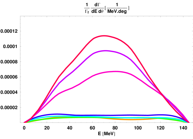
Figure 3: The same as in Fig. 2, but for neutron kinetic energy spectra, $T_{n}\equiv E$, of the $\Lambda n\to nn$ decay channel.

The kinetic energy spectra ${\rm d}\Gamma_{p,n}/{\rm d}E$, for the proton and neutron-induced decay channels, integrated over the relative angle $\theta$, are presented in Fig. 4. The results obtained with only OPE and with $\pi+K$ exchange are compared in the figure. The $PV{{}^{\prime}}$ choice for the vertices has been adopted in the calculations, and both initial and final SRC are included. In the OPE case the proton spectrum is significantly larger in size than the neutron one. Moreover, the two-peak structure is evident in the proton spectrum, while the shape of the neutron spectrum is smoother and much more symmetric with respect to $T_{max}/2$. The inclusion of the OKE contribution produces a more peaked proton spectrum but does not modify its global size. In contrast, the neutron spectrum is considerably reduced by OKE and its shape is slightly flattened. At the level of integrated observables, such a behaviour produces the reduction of the $\Gamma_{n}/\,\Gamma_{p}$ ratio, when including kaon-exchange. In Fig. 5 the kinetic energy spectra integrated over $\theta$ are given for $PS$ couplings. The proton spectrum with only OPE again shows an asymmetric shape, with a slight two-peak behaviour (its global scale is now about twice the one for the corresponding $PV{{}^{\prime}}$ case). The inclusion of the OKE contribution yields an almost identical shape but reduces the global size of the proton spectrum. The neutron energy spectrum for the OPE case is smoother and smaller in size with respect to the proton one. When we include the OKE contribution, the neutron spectrum becomes much more peaked and its size is increased. These results are in opposite trend with respect to what found for $PV{{}^{\prime}}$ couplings in Fig. 4 and, by consequence, in the $PS$ case the $\Gamma_{n}/\,\Gamma_{p}$ is considerably increased by the addition of the OKE mechanism and becomes larger than 0.6 (see Table 2).

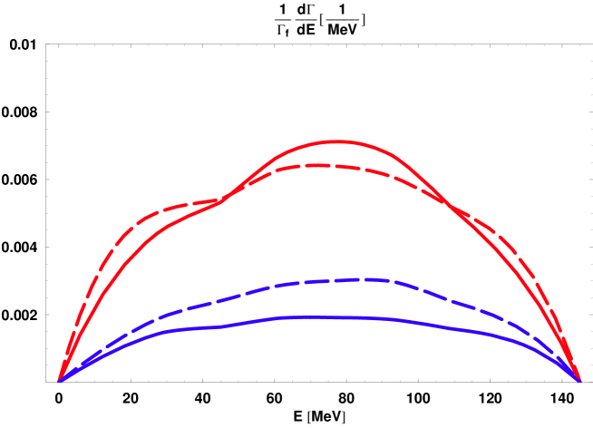
Figure 4: Kinetic energy spectra (normalized to $\Gamma_{\Lambda}^{free}$) integrated over the angle $\theta$. Calculations are performed with $PV{{}^{\prime}}$ couplings and include both initial and final SRC. Red (blue) lines refer to proton (neutron) spectra, as obtained in proton-(neutron-)induced one-body decay channels ($E\equiv T_{p,n}$). Dashed lines correspond to results obtained with only OPE, solid lines are obtained including also OKE contributions.

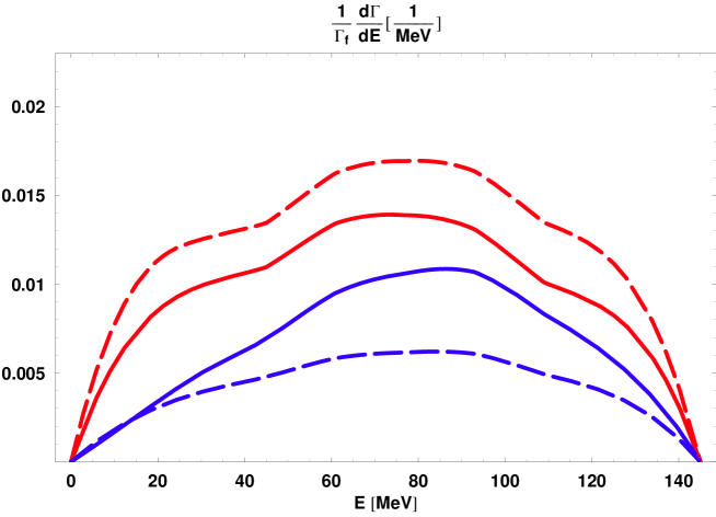
Figure 5: The same in Fig. 4, but for $PS$ couplings.

Similar analyses can also be repeated for the corresponding model configurations in which either final SRC or both initial and final SRC contributions are neglected. The shapes of the spectra are quite insensitive to the presence or absence of short range correlations, as implemented in our model. On the other hand, the global size of the spectra and the corresponding integrated quantities $\Gamma_{p,n}$ are influenced, sometimes significantly, by SRC effects.

III.3 Angular spectra

In this Section we analyze the angular distributions predicted by our model. In Figs. 6-7 the double-differential spectra, ${\rm d}\Gamma_{p,n}/{\rm d}E\,{\rm d}\theta$, for the $\Lambda p\to np$ and $\Lambda n\to nn$ decay channels at different values of the proton and neutron kinetic energy, $T_{p,n}\equiv E$, are displayed as a function of the relative angle $\theta$ between the momenta of the two outgoing nucleons. The spectra are calculated with $PV{{}^{\prime}}$ vertices, including both OPE and OKE contributions as well as initial and final SRC. The angular spectra for proton- and neutron-induced channels exhibit a similar behavior. In both figures all the curves, corresponding to different values of the kinetic energy of the outgoing nucleon, are strongly peaked at high angles, especially for $150^{o}\leq\theta\leq 180^{o}$. This agrees with the fact that the elementary process driving the decay is a two-body $\Lambda N\to nN$ interaction, which preferentially yields back-to-back final nucleons. Distortion effects produced by the nucleon-nucleus optical potential, however, tend to smear the angular distributions, thus increasing the probability of emitting nucleons in non back-to-back configurations and at small angles. In the angular region between $0^{o}$ and $120^{o}$ all the spectra have similar shapes and comparable sizes, while in the back-to-back region they suddenly increase and differentiate among each others. The angular spectra associated with central energies (52, 68, 84 MeV) display a higher peak, while the curves obtained for energies close to the energy endpoints (20 and 128 MeV) are much less peaked and definitely smaller in size.

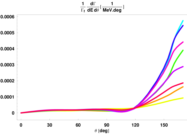
Figure 6: Double-differential spectra (normalized to $\Gamma_{\Lambda}^{free}$) for the $\Lambda p\to np$ decay channel as a function of the relative angle $\theta$ between the momenta of the two outgoing nucleons for different values of the kinetic energy of the outgoing proton $T_{p}\equiv E$. Line convention: $E=20$ MeV (orange), $E=36$ MeV (green), $E=54$ MeV (cyan), $E=68$ MeV (blue), $E=84$ MeV (magenta), $E=100$ MeV (purple), $E=116$ MeV (red), $E=128$ MeV (yellow). Calculations are performed with $PV{{}^{\prime}}$ couplings and include $\pi+K$ contributions as well as initial and final SRC.

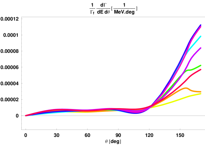
Figure 7: The same as in Fig. 6, but for neutron angular spectra of the $\Lambda n\to nn$ decay channel.

The evidence that the most back-to-back peaked angular spectra are those pertaining to central energies can be understood if we observe that a proton or a neutron kinetic energy close to the middle of the available energy range means that the two final nucleons have approximately the same energy. Thus, due to the energy-momentum global conservation in the two-body process, the two outgoing particles are preferentially emitted along opposite directions. On the other hand, in those cases in which one of the two nucleons carries away a large part of the available energy and the other one carries the remaining small amount, the angular correlation is weaker and the corresponding angular spectra are flatter. The angular distributions are smeared by FSI effects. The complex energy dependent optical potential distorts the wave functions of the outgoing nucleons and an imbalance between the energies of the two final nucleons also favours a weakening of their angular correlation and a correspondingly stronger smearing of the relative angle distribution.

The angular spectra integrated over the kinetic energy of the outgoing proton (for the $\Lambda p\to np$ channel) and neutron (for the $\Lambda n\to nn$ channel), ${\rm d}\Gamma_{p,n}/{\rm d}{\theta}$, are shown in Fig. 8. The results obtained with OPE and $\pi+K$ exchange are compared in the figure. Calculations have been performed adopting the $PV{{}^{\prime}}$ choice for the vertices and include both initial and final SRC. By considering only the OPE mechanism we see that the proton and neutron angular distributions are quite similar in shape, especially in the back-to-back region, namely from $\theta=120^{o}-130^{o}$ till $\theta=180^{o}$, where they present similar peaks. In the region where $\theta\leq 120^{o}$ the angular spectra are instead approximately flat and strongly reduced in size. The global size of the proton spectrum is about twice the neutron spectrum one, coherently with the obtained results for the ratio of the integrated decay rates, $\Gamma_{n}/\,\Gamma_{p}$. The inclusion of the OKE contribution acts in opposite ways on the proton and neutron spectra. The curves are practically unchanged in the region $\theta\leq 120^{o}$, apart from a slight reduction of the proton spectrum. By contrast, in the back-to-back region, the neutron spectrum is considerably lowered and flattened while the proton spectrum is correspondingly increased, becoming much more peaked towards higher relative angles. This behaviour produces the reduction of the $\Gamma_{n}/\Gamma_{p}$ ratio shown in Table 2, when the OKE contribution is included.

The angular spectra integrated over the kinetic energy of the outgoing proton and neutron calculated with $PS$ couplings (and including initial and final SRC) are shown in Fig. 9. Also in this case the OPE spectra have similar shapes, with the neutron curve significantly smaller than the proton one in the back-to-back region. On the contrary, the inclusion of the OKE mechanism induces opposite effects on the angular spectra, when considering $PS$ and $PV{{}^{\prime}}$ vertices: in the $PS$ case the proton distribution is reduced and the neutron one is strongly increased. Thus, the $\Gamma_{n}/\,\Gamma_{p}$ ratio is highly enhanced and becomes greater than 0.6 (see Table 2).

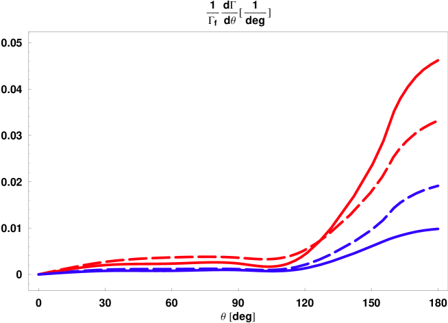
Figure 8: Angular spectra (normalized to $\Gamma_{\Lambda}^{free}$) integrated over the nucleon kinetic energy $E\equiv T_{N}$. Calculations are perfomed with $PV{{}^{\prime}}$ couplings and include initial and final SRC. Red (blue) lines refer to proton (neutron) spectra, as obtained in proton- (neutron-) induced one-body decay channels. Dashed lines correspond to results obtained by considering only OPE, solid ones are obtained including also OKE contributions.

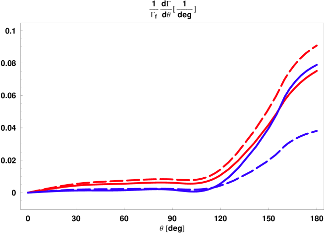
Figure 9: The same in Fig. 8, but for $PS$ couplings.

A similar analysis can be repeated for the model configurations in which SRC are completely neglected. The shapes and the relative sizes of the distributions are strictly analogous to the corresponding results obtained when SRC are included. The conclusion is that, within our model, SRC do not affect in a significant way the shapes and sizes of kinetic energy and angular spectra. This is coherent with the use of a phenomenological SRC multiplicative, local and energy-independent function.

IV Summary and conclusions

We have presented a relativistic model for the non-mesonic weak decay of the ${}^{12}_{\Lambda}C$ hypernucleus. Over the last years many groups have been deeply involved in studies of hypernuclear physics and developed different nonrelativistic models that can satisfactorily reproduce all the experimental results. Anyway, the inclusion of many theoretical ingredients, like the full one-meson-exchange potential and many other ones, seems mandatory. In this paper we have proposed a first attempt to explain, at least in a qualitative way, all the features of the hypernuclear non-mesonic weak decay with a fully relativistic treatment of the weak dynamics, based on the evaluation of Feynman diagrams within a covariant formalism.

We have considered the pseudo-scalar and pseudo-vector prescriptions for the weak-strong vertices involved in the $\Lambda N\to nN$ elementary process. When considering the standard form of the pseudo-vector vertex, these two different couplings produce the same nonrelativistic limit, which is anyway inconsistent with the standard nonrelativistic approaches; only the modified pseudo-vector vertex, with a 4-derivative $\partial_{\mu}$ operating on the meson propagator, allows to obtain, in the nonrelativistic limit, the usual one-pion-exchange potential commonly employed in nonrelativistic calculations. In view of such considerations, we tested our model employing both pseudo-scalar and modified derivative pseudo-vector couplings. In our model short-range correlations are taken into account in a phenomenological way, through a multiplicative local and energy-independent function. The involved wave functions are 4-spinors obtained within the framework of Dirac phenomenology in presence of scalar and vector potentials. Final-state interactions are included in the model by accounting for the interaction of each one of the two outgoing nucleons with the residual nucleus, that is implemented by means of a complex relativistic nucleon-nucleus optical potential. The main effect of the optical potentials is to produce a damping of the kinetic energy and angular spectra and to smear the two-body reaction kinematical correlations.

Great care has been devoted to the decay dynamics. The pseudo-vector couplings yield predictions in reasonable agreement with the non-mesonic weak decay experimental rates, whereas visible discrepancies appear when the pseudo-scalar coupling is chosen. The role of one-pion-exchange and one-kaon-exchange diagrams has been carefully investigated. When using pseudo-vector couplings, the inclusion of the $K$-exchange is helpful in view of a comparison with the experimental determinations of the $\Gamma_{n}/\Gamma_{p}$ ratio. On the contrary, if we adopt the pseudo-scalar vertices, the $K$-exchange gives puzzling big values.

The role of initial short-range correlations is only moderate and especially visible in the total decay rates, which are reduced by about 20-25%, whereas $\Gamma_{n}/\Gamma_{p}$ is much less sensitive to such a theoretical ingredient. The additional consideration of final SRC does not seem to introduce significant modifications, when initial SRC are already taken into account. We acknowledge that the particular implementation of SRC here adopted, namely in terms of local multiplicative functions inspired by non-relativistic calculations, could be unsuitable in the context of a fully relativistic calculation. Our choice to include such ingredients has been motivated by the relevance usually attributed to these correlations in non-relativistic hypernuclear decay calculations; the great care here devoted to the problem of selecting the right covariant vertices structure in combination with these non-relativistic SRC functions was actually aimed at minimizing the impact of the theoretical uncertainty introduced by such phenomenological inputs. Clearly, modeling short range baryon-baryon correlations directly in the relativistic framework, e.g. by considering box diagrams involving heavy mesons (typically the $\omega$), would definitely be a better strategy, though much more demanding from a calculational viewpoint: we believe this topic deserves deeper investigation and our calculation can be a starting point in view of similar generalizations.

In contrast with the predictions of nonrelativistic calculations, our model produces significantly high values of the $\Gamma_{n}/\Gamma_{p}$ ratio, especially when we only include the one-pion-exchange contribution. As a consequence, our results for $\Gamma_{n}/\Gamma_{p}$, both for $\pi$-and $(\pi+K)$-exchange contributions, are close to the experimental measurements, without any apparent need to include other pseudo-scalar and vector mesons, that are usually accounted for by the full OME models, or to resort to more refined FSI models.

It is not easy to understand why the obtained results are so different from well-established non-relativistic predictions. Due to the high energies involved and short distances probed, the role of relativity could really be important in hypernuclear non-mesonic weak decay; unfortunately, no work to date could demonstrate this point with certainty. A direct comparison between our model and standard nonrelativistic calculations is beyond the scope of the present investigation, also because it would be very difficult to establish the basis for a direct and unambiguous comparison. A nonrelativistic reduction would imply first of all to drop the lower components of the Dirac spinors and apply the proper normalization. In addition, the relativistic energy $E$ should be put equal to $M$. However, this is by no means a nonrelativistic reduction, as relativity is directly included in the vertices and the propagators of the Feynman diagrams, and the nuclear current operators still involve the Dirac scalar and vector potentials, which can produce large differences between the results.

We are aware that, at the present stage of development of our work, we cannot derive any definite conclusion about the relevance or the usefulness of a fully relativistic formalism to describe the short-range strong-weak dynamical mechanism driving hypernuclear non-mesonic decay. We are considering the opportunity to better describe the final state of the decay process, by refining the treatment of short-range strong correlations between the two outgoing nucleons, here simply described by means of a phenomenological non-relativistic function, and thus evaluating a globally correlated relativistic wave function for the final nucleon pair. Another possible improvement is related to the dynamics of the model, and requires the implementation of the exchange of vector mesons, thus exploring the effects of these additional contributions on the integrated observables and on the simulated spectra. Anyway, we think that the results of our model represent an additional source of information and a partly new theoretical perspective, which may deserve attention and further investigation.

References

References

- (1) M. Danysz and J. Pniewski, Philos. Mag. 44 (1953) 348 .
- (2) E. Oset and A. Ramos, Prog. Part. Nucl. Phys. 41 (1998) 191.
- (3) W.M. Alberico and G. Garbarino, Phys. Rep. 369 (2002) 1.
- (4) W.M. Alberico and G. Garbarino, in Hadron Physics, IOS Press, Amsterdam, 2005, p. 125. Edited by T. Bressani, A. Filippi and U. Wiedner Proceedings of the International School of Physics ”Enrico Fermi”, Course CLVIII, Varenna (Italy), June 22 - July 2, 2004 [nucl-th/0410059].
- (5) H, Outa in Hadron Physics, IOS Press, Amsterdam, 2005, p.219. Edited by T. Bressani, A. Filippi and U. Wiedner Proceedings of the International School of Physics ”Enrico Fermi”, Course CLVIII, Varenna (Italy), June 22 - July 2, 2004 [nucl-th/0410059].
- (6) G. Garbarino, Proceedings of the IX International Conference on Hypernuclear and Strange Particle Physics HYP 2006, Edited by J. Pochidzalla and T. Walcher, Springer 2007 p.107 [nucl-th/0701949].
- (7) A. Parreo, Lecture Notes Phys. 724 (2007) 141.
- (8) C. Chumillas, G. Garbarino, A. Parreo, A. Ramos, Nucl. Phys. A 804 (2008) 162.
- (9) K. Itonaga, T. Ueda and T. Motoba, Nucl. Phys. A 639 (1998) 329c.
- (10) K. Itonaga, T. Ueda and T. Motoba, Nucl. Phys. A 577 (1994) 301c.
- (11) A. Parreo and A. Ramos, Phys. Rev. C 65 (2002) 015204.
- (12) T. Inoue, M. Oka, T. Motoba and K. Itonaga, Nucl. Phys. A 633 (1998) 312.
- (13) A. Parreo, A. Ramos and C. Bennhold, Phys. Rev. C 56 (1997) 339.
- (14) K. Itonaga, T. Ueda and T. Motoba, Phys. Rev. C 65 (2002) 034617.
- (15) D. Jido, E. Oset and J.E. Palomar, Nucl. Phys. A 694 (2001) 525.
- (16) J.F. Dubach, G. B. Feldman, B.R. Holstein and L. de la Torre, Nucl. Phys. A 450 (1986) 71c.
- (17) J.F. Dubach, G. B. Feldman and B.R. Holstein, Ann. Phys. 249 (1996) 146.
- (18) M. Shmatikov, Nucl Phys. A 580 (1994) 538.
- (19) K. Maltman and M. Shmatikov, Phys. Lett. B 331 (1994) 1; Nucl. Phys. A 585 (1995) 343c.
- (20) K. Maltman and M. Shmatikov, Phys. Rev. C 51 (1995) 1576.
- (21) A. Parreo, A. Ramos, C. Bennhold and K. Maltman, Phys. Lett. B 435 (1998) 1.
- (22) C.-Y. Cheung, D.P. Heddle and L.S. Kisslinger, Phys. Rev. C 27 (1983) 335; D.P. Heddle and L.S. Kisslinger, Phys. Rev. C 33 (1986) 608.
- (23) T. Inoue, S. Takeuchi and M. Oka, Nucl. Phys. A 597 (1996) 563.
- (24) K. Sasaki, T. Inoue and M. Oka, Nucl. Phys. A 669 (2000) 331; A 678 (2000) 455(E); A 707 (2002) 477.
- (25) J.H. Kim et al., Phys. Rev. C 68 (2003) 065201.
- (26) S. Okada et al., Phys. Lett. B 597 (2004) 249.
- (27) H. Outa et al., Nucl. Phys. A 754 (2005) 157c.
- (28) B.H. Kang et al., Phys. Rev. Lett. 96 (2006) 062301.
- (29) S. Okada et al., Nucl.Phys. A 752 (2005) 196.
- (30) M.J. Kim et al., Phys. Lett. B 641 (2006) 28.
- (31) M. Agnello et al., Phys. Lett. B 685 (2010) 247.
- (32) G. Garbarino, A. Parreo and A. Ramos, Phys. Rev. Lett. 91 (2003) 112501.
- (33) G. Garbarino, A. Parreo and A. Ramos, Phys. Rev. C 69 (2004) 054603.
- (34) C. Barbero, C. De Conti, A. P. Galeo and F. Krmpotic, Nucl. Phys. A 726 (2003) 267.
- (35) E. Bauer and F. Krmpotic, Nucl. Phys. A 717 (2003) 217; E. Bauer A 739 (2004) 109.
- (36) J.H. Jun and H.C. Bhang, Nuovo Cim. 112 A (1999) 649; J.H. Jun, Phys. Rev. C 63 (2001) 044012.
- (37) A. Parreo, C. Bennhold and B.R. Holstein, Phys. Rev. C 70 051601(R) (2004).
- (38) E. Bauer, G. Garbarino, A. Parreo and A. Ramos, nucl-th/0602066.
- (39) F. Krmpoti, Phys. Rev. C 82 (2010) 055204;
- (40) E. Bauer, A.P. Galeao, M.S. Hussein and F. Krmpotic, Nucl. Phys. A 834 (2010) 599C.
- (41) A. Feliciello, Nucl. Phys. A 691 (2001) 170c.
- (42) S. Ajimura, Precise measurement of the non-mesonic weak decay of =4,5 -hypernuclei, Letter of intent (LOI21) for experiments at J-PARC (2003).
- (43) S. Ajimura et al., Phys. Lett. B 282 (1992) 293.
- (44) S. Ajimura et al., Phys. Rev. Lett. 84 (2000) 4052.
- (45) H. Band, T. Motoba M. Sotona and J. Zofka, Phys. Rev. C 39 (1989) 587.
- (46) A. Ramos, E. van Meijgaard, C. Bennhold and B.K. Jennings, Nucl. Phys. A 544 (1992) 703.
- (47) T. Maruta et al., Nucl. Phys. A 754 (2005) 168c.
- (48) T. Maruta, PhD thesis, KEK Report 2006-1 (2006).
- (49) W. M. Alberico, G. Garbarino, A. Parreo and A. Ramos, Phys. Rev. Lett. 94 (2005) 082501.
- (50) C. Chumillas, G. Garbarino, A. Parreo and A. Ramos, Phys. Lett. B 657 180 (2007).
- (51) E. Oset and L. L. Salcedo, Nucl. Phys. A 443 (1985) 704.
- (52) E. Oset, P. Fernandez de Cordoba, J. Nieves, A. Ramos and L.L. Salcedo, Prog. Theor. Phys. Suppl. 117 (1994) 461.
- (53) A. Ramos, M.J. Vicente-Vacas, and E. Oset, Phys. Rev. C 55 (1997) 735.
- (54) A. Ramos, M.J. Vicente-Vacas, and E. Oset, Phys. Rev. C 66 (2002) 039903, Erratum of Ref. ICC .
- (55) Y. Sato et al., Phys. Rev. C 71 (2005) 025203.
- (56) A. Ramos, E. Oset and L.L Salcedo, Phys. Rev. C 50 (1994) 2314.
- (57) P. Fernandez de Cordoba, E. Oset, M.J. Vicente-Vacas, Yu. Ratis, J. Nieves, B. Lopez-Alvaredo, and F. Gareev, Nucl. Phys. A 586 (1995) 586.
-
(58)
F. Conti, PhD thesis, University of Pavia (2009). Electronic format available upon request: please contact the author at
francesco.conti@pv.infn.it. - (59) H. Band, Prog. Theor. Phys. Suppl. No. 81 (1985) 181.
- (60) D. Halderson, Phys. Rev. C 48 (1993) 581.
- (61) A. Parreo, A. Ramos, and E. Oset, Phys. Rev. C 51 (1995) 2477.
- (62) W. Weise, Nucl. Phys. A 278, (1977) 402.
- (63) R. V. Reid, Ann. Phys. N.Y. 50, (1968) 411.
- (64) L. Zhou and J. Piekarewicz, Phys. Rev. C60 (1999) 024306.
- (65) C. Bennhold, A. Parreo and A. Ramos, Phys. Rev. C 56 (1997) 1.
- (66) E.H. Auerbach, A.J. Baltz, C.B. Dover, A. Gal, S.H. Kahana, L. Ludeking, and D.J. Millener, Ann. of Phys. (N.Y.) 148 (1983) 381.
- (67) P.M.M. Maessen, Th.A. Rijken, and J.J. de Swart, Phys. Rev. C 40 (1989) 2226.
- (68) C.J. Horowitz and B.D. Serot, Nucl. Phys. A 368 (1981) 503; Phys. Lett. B 86 (1979) 146.
- (69) B.D. Serot and J.D. Walecka, Adv. Nucl. Phys. 16 (1986) 1.
- (70) W. Pöschl, D. Vretenar, and P. Ring, Comput. Phys. Commun. 103 (1997) 217.
- (71) G.A. Lalazissis, J. König, and P. Ring, Phys. Rev. C 55 (1997) 540.
- (72) M.M. Sharma, M.A. Nagarajan, and P. Ring, Phys. Lett. B 312 (1993) 377.
- (73) B.C. Clark, in Proceedings of the Workshop on Relativistic Dynamics and Quark-Nuclear Physics, edited by M.B. Johnson and A. Picklesimer (John Wiley & Sons, New York, 1986), p. 302; E.D. Cooper, S. Hama, B.C. Clark, and R.L. Mercer, Phys. Rev. C 47 (1993) 297.
- (74) S. Boffi, C. Giusti, F.D. Pacati, and M. Radici, Electromagnetic Response of Atomic Nuclei, Oxford Studies in Nuclear Physics, Vol. 20 (Clarendon Press, Oxford, 1996); S. Boffi, C. Giusti, and F.D. Pacati, Phys. Rep. 226 (1993) 1.
- (75) J.J. Kelly, Adv. Nucl. Phys. 23 (1996) 75.
- (76) J.M. Udías, P. Sarriguren, E. Moya de Guerra, E. Garrido, and J.A. Caballero, Phys. Rev. C 48 (1993) 2731; C 51 (1995) 3246.
- (77) J.M. Udías, P. Sarriguren, E. Moya de Guerra, and J.A. Caballero, Phys. Rev. C 53 (1996) R1488.
- (78) J.M. Udías, J.A. Caballero, E. Moya de Guerra, J.R. Vignote, and A. Escuderos, Phys. Rev. C 64 (2001) 024614.
- (79) A. Meucci, C. Giusti, and F.D. Pacati, Phys. Rev. C 64, (2001) 014604.
- (80) A. Meucci, C. Giusti, and F.D. Pacati, Phys. Rev. C 64 (2001) 064615.
- (81) A. Meucci, Phys. Rev. C 65 (2002) 044601.
- (82) A. Meucci, C. Giusti, and F.D. Pacati, Phys. Rev. C 66 (2002) 034610.
- (83) M. Radici, A. Meucci, and W.H. Dickhoff, Eur. Phys. J. A 17 (2003) 65.
- (84) A. Meucci, F. Capuzzi, C. Giusti, and F.D. Pacati, Phys. Rev. C 67 (2003) 054601.
- (85) A. Meucci, C. Giusti, and F.D. Pacati, Nucl. Phys. A 739 (2004) 277.
- (86) A. Meucci, C. Giusti, and F.D. Pacati, Nucl. Phys. A 756 (2005) 359.
- (87) A. Meucci, C. Giusti, and F.D. Pacati, Nucl. Phys. A 773 (2006) 250.
- (88) M. Kim et al., Phys. Rev. Lett. 103 (2009) 182502.
- (89) S. Okada et al., Nucl.Phys. A 754 (2005) 178.
- (90) M. Hedayati-Poor and H. S. Sherif, Phys. Lett. B (1994) 326 and Phys. Rev. C 51 (1995) 2044