Physical Properties of (2) Pallas

Abstract

Ground-based high angular-resolution images of asteroid (2) Pallas at near-infrared wavelengths have been used to determine its physical properties (shape, dimensions, spatial orientation and albedo distribution).
We acquired and analyzed adaptive-optics (AO) J/H/K-band observations from Keck II and the Very Large Telescope taken during four Pallas oppositions between 2003 and 2007, with spatial resolution spanning 32–88 km (image scales 13–20 km/pix). We improve our determination of the size, shape, and pole by a novel method that combines our AO data with 51 visual light-curves spanning 34 years of observations as well as archived occultation data.
The shape model of Pallas derived here reproduces well both the projected shape of Pallas on the sky (average deviation of edge profile of 0.4 pixel) and light-curve behavior (average deviation of 0.019 mag) at all the epochs considered. We resolved the pole ambiguity and found the spin-vector coordinates to be within 5^∘ of [long, lat] = [30^∘, -16^∘] in the Ecliptic J2000.0 reference frame, indicating a high obliquity of about 84^∘, leading to high seasonal contrast. The best triaxial-ellipsoid fit returns ellipsoidal radii of $a$=275 km, $b$= 258 km, and $c$= 238 km. From the mass of Pallas determined by gravitational perturbation on other minor bodies [(1.2 $\pm$ 0.3) $\times$ 10^-10 M_⊙, Michalak 2000, A&A, 360], we derive a density of 3.4 $\pm$ 0.9 g.cm^-3 significantly different from the density of C-type (1) Ceres of 2.2 $\pm$ 0.1 g.cm^-3 [Carry et al. 2008, A&A, 478]. Considering the spectral similarities of Pallas and Ceres at visible and near-infrared wavelengths, this may point to fundamental differences in the interior composition or structure of these two bodies.
We define a planetocentric longitude system for Pallas, following IAU guidelines. We also present the first albedo maps of Pallas covering $\sim$80% of the surface in K-band. These maps reveal features with diameters in the 70$-$180 km range and an albedo contrast of about 6% with respect to the mean surface albedo.

1 Introduction

A considerable amount of information regarding the primordial planetary processes that occurred during and immediately after the accretion of the early planetesimals is still present among the population of small solar system bodies (Bottke et al., 2002).
Fundamental asteroid properties include composition (derived from spectroscopic analysis) and physical parameters (such as size, shape, mass, and spin orientation). While compositional investigations can provide crucial information on the conditions in the primordial solar nebula (Scott, 2007) and on asteroid thermal evolution (Jones et al., 1990), the study of asteroid physical properties can yield insights on asteroid cratering history (Davis, 1999), internal structure (Britt et al., 2002), and volatile fraction (Mousis et al., 2008) for example. These approaches complement one another — the density derived by observations of physical properties strongly constrains the composition (Merline et al., 2002), which is key to evaluation of evolution scenarios.
Spacecraft missions to asteroids, for example NEAR to (253) Mathilde and (433) Eros (Veverka et al., 1999), and Hayabusa to (25143) Itokawa (Fujiwara et al., 2006), greatly enhanced our understanding of asteroids. The high cost of space missions, however, precludes exploration of more than a few asteroids, leaving most asteroids to be studied from Earth-based telescopes.
Although several remote observation techniques can be used to determine the physical properties of asteroids, our technique relies primarily on disk-resolved observations. Indeed, knowing accurately the size is crucial for the determination of asteroid volume, and hence density. If enough chords are observed, occultations provide precise measurement of asteroid shape and size (Millis and Dunham, 1989), but at only one rotational phase (per occultation event). Moreover, because occultations of bright stars seldom occur, only a small fraction of all occultations are covered by a significant number of observers. Describing an asteroid’s 3-D size and shape with this method thus requires decades. Assuming a tri-axial ellipsoidal shape is a common way to build upon limited observations of asteroid projected sizes (Drummond and Cocke, 1989). From the inversion of photometric light-curves, one can also derive asteroid shapes (Kaasalainen et al., 2002), with sizes then relying on albedo considerations. On the other hand, disk-resolved observations, either radar or high angular-resolution imagery, provide direct measurement of an asteroid’s size and shape when its apparent disk can be spatially resolved.
For about a decade now, we have had access to instrumentation with the angular resolution required to spatially resolve large main-belt asteroids at optical wavelengths. This can be done in the visible from space with the Hubble Space Telescope (HST) or in near-infrared from large telescopes equipped with adaptive optics (AO) such as Keck, the Very Large Telescope (VLT), and Gemini. Disk-resolved observations allow direct measurement of an asteroid’s absolute size (Saint-Pé et al., 1993a), and of its shape, if enough rotational-phase coverage is obtained (Taylor et al., 2007; Conrad et al., 2007). One can also derive the spin-vector coordinates from the time evolution of limb contours (Thomas et al., 2005) or from the apparent movement of an albedo feature (Carry et al., 2008). Ultimately, albedo maps may provide significant constraints on surface properties such as mineralogy or degree of space weathering (Binzel et al., 1997; Li et al., 2006; Carry et al., 2008).
Even if images can provide a complete description of asteroid properties, their combination with other sources of data (like light-curves or occultations) can significantly improve asteroid 3-D shape models (see the shape model of (22) Kalliope in Descamps et al., 2008, for instance).
Pallas is a B-type asteroid (Bus and Binzel, 2002). As such, it is thought to have a composition similar to that of the Carbonaceous Chondrite (CC) meteorites (see Larson et al., 1983, for a review). Spectral analysis of the 3 micron band (Jones et al., 1990) exhibited by Pallas suggests that its surface has a significant anhydrous component mixed with hydrated CM-like silicates (CM is a subclass of CC meteorites). Although Pallas is generally linked to CC/CM material, its composition remains uncertain. Indeed, Pallas’ visible and near-infrared spectrum is almost flat with only a slight blue slope, with the only absorption band clearly detected being the 3 micron band.
Compositional/mineralogical studies for Pallas are further hampered by a poorly determined density. First, there is significant uncertainty in the mass, as most mass estimates do not overlap within the error bars (see Hilton, 2002, for a review). Second, although the size of Pallas has been estimated from two occultations (Wasserman et al., 1979; Dunham et al., 1990), at least three events are required to determine asteroid spin and tri-axial dimensions (Drummond and Cocke, 1989).
Until recently, the only published disk-resolved observations of Pallas were limited to some AO snapshots collected in 1991 by Saint-Pé et al. (1993b), but the lack of spatial resolution prevented conclusions about Pallas’ size, shape, or spatial orientation. Recent observations of Pallas from Lick (Drummond and Christou, 2008) and Keck Observatories (Drummond et al., 2009) lead to new estimates for its triaxial ellipsoid dimensions, but there was still a relatively large uncertainty on the short axis. These Keck observations are included as a subset of the data considered here. Also, observations of Pallas were recently obtained using the WFPC2 instrument on HST (see Schmidt et al., 2009).

2 Observations

Here we present high angular-resolution images of asteroid (2) Pallas, acquired at multiple epochs, using AO in the near infrared with the Keck II telescope and the ESO Very Large Telescope (VLT).
During the 2003, 2006 and 2007 oppositions, we imaged Pallas in Kp-band [central wavelengths and bandwidths for all bands are given in Table 2] with a 9.942 $\pm$ 0.050 milliarcsec per pixel image scale of NIRC2, the second generation near-infrared camera (1024$\times$1024 InSb Aladdin-3) and the AO system installed at the Nasmyth focus of the Keck II telescope (van Dam et al., 2004). We acquired five other epochs near the more favorable 2005 opposition during which we imaged Pallas in J-, H-, and Ks-bands, with the 13.27 $\pm$ 0.050 milliarcsec per pixel image scale of CONICA (1024$\times$1026 InSb Aladdin-3) (Rousset et al., 2003; Lenzen et al., 2003) and the NAOS AO system installed at the Nasmyth B focus of UT4/Yepun at the VLT. We list in Table 1 Pallas’ heliocentric distance and range to observer, phase angle, angular diameter and Sub-Earth-Point (SEP, with planetocentric coordinate system defined in section 5.1) coordinates for each observation.
Near-infrared broad-band filter observations of Pallas were interspersed with observations of a Point-Spread-Function (PSF) reference star at similar airmass and through the same set of filters (Tables 2 & 3). This calibration was required to perform a posteriori image restoration (deconvolution) as described in Carry et al. (2008). These observations of stars also can be used to measure the quality of the AO correction during the observations. We thus report in Table 3 the Full Width at Half Max (FWHM) of each PSF, in milliarcseconds and also in kilometers at the distance of Pallas. No offset to sky was done, but the telescope position was dithered after one or a few exposures to place the object (science or calibration) at three different locations on the detector separated by $\sim$5^′′ from each other. This allows a median sky frame to be created directly from the acquired targeted images.

Observation Conditions
Date UT $\Delta$ $r$ V $\alpha$ $\phi$ SEP_λ SEP_φ Airmass PSF (AU) (AU) (mag.) (^∘) (^′′) (^∘) (^∘) (Table 3) 2003 Oct 10 12:00 2.73 1.80 8.25 09.4 0.39 107 -76 1.28 Oct.10-$\star$1 2003 Oct 12 09:13 2.73 1.80 8.24 09.5 0.39 183 -75 1.40 Oct.12-$\star$1 2003 Oct 12 11:14 2.73 1.80 8.24 09.5 0.39 090 -75 1.25 Oct.12-$\star$2 2005 Feb 02 06:30 2.27 1.60 8.04 21.9 0.44 265 +64 1.21 Feb.02-$\star$1 2005 Feb 02 08:05 2.26 1.60 8.04 21.9 0.49 192 +64 1.05 Feb.02-$\star$2 2005 Mar 12 06:02 2.34 1.37 7.20 06.9 0.52 054 +64 1.15 Mar.12-$\star$ 2005 Mar 13 04:42 2.34 1.37 7.18 06.6 0.52 090 +64 1.21 Mar.13-$\star$ 2005 May 08 23:30 2.47 1.77 8.39 20.1 0.40 326 +54 1.74 May.08-$\star$1 2005 May 09 23:18 2.47 1.78 8.41 20.3 0.40 309 +54 1.80 May.09-$\star$1 2006 Aug 16 06:55 3.35 2.76 9.85 15.5 0.26 022 +32 1.00 Aug.16-$\star$1 2006 Aug 16 07:22 3.35 2.76 9.85 15.5 0.26 001 +32 1.01 Aug.16-$\star$1 2006 Aug 16 07:45 3.35 2.76 9.85 15.5 0.26 343 +32 1.03 Aug.16-$\star$1 2006 Aug 16 08:12 3.35 2.76 9.85 15.5 0.26 322 +32 1.07 Aug.16-$\star$2 2006 Aug 16 08:45 3.35 2.76 9.86 15.5 0.26 297 +32 1.13 Aug.16-$\star$2 2006 Aug 16 09:00 3.35 2.76 9.86 15.5 0.26 285 +32 1.17 Aug.16-$\star$3 2006 Aug 16 09:18 3.35 2.76 9.86 15.5 0.26 272 +32 1.23 Aug.16-$\star$3 2007 Jul 12 13:15 3.31 2.69 9.78 15.5 0.26 211 -38 1.03 Jul.12-$\star$ 2007 Nov 01 04:30 3.16 2.64 9.68 16.9 0.27 265 -27 1.19 Nov.01-$\star$ 2007 Nov 01 06:06 3.16 2.64 9.68 16.9 0.27 191 -27 1.12 Nov.01-$\star$

Table 1: Heliocentric distance ($\Delta$) and range to observer ($r$), visual magnitude (V), phase angle ($\alpha$), angular diameter ($\phi$), and Sub-Earth-Point (SEP) coordinates (longitude $\lambda$ and latitude $\varphi$) for each epoch (given in UT, the mid-observation time, here listed without light-time correction, although light-time corrections are included in all relevant computations in this paper). Airmass at the tabulated UT is also reported. The last column is a tag for the PSF used for deconvolution; see Table 3 for a complete description of the stars.

Observation Settings
Date Inst. Filters $\lambda_{c}$ $\Delta\lambda$ Images $\Theta$ ROI (UT) ($\mu$m) ($\mu$m) # (km) (%) 2003 Oct 10^a NIRC2 Kp 2.124 0.35 04 57 60 2003 Oct 12^b NIRC2 Kp 2.124 0.35 09 57 60 2005 Feb 02^a NACO J 1.265 0.25 08 37 60 2005 Feb 02^a NACO H 1.66 0.33 12 48 55 2005 Feb 02^a NACO Ks 2.18 0.35 13 64 50 2005 Mar 12^a NACO J 1.265 0.25 06 32 60 2005 Mar 12^a NACO H 1.66 0.33 06 41 60 2005 Mar 12^a NACO Ks 2.18 0.35 05 54 60 2005 Mar 13^a NACO J 1.265 0.25 06 32 60 2005 Mar 13^a NACO H 1.66 0.33 06 41 60 2005 Mar 13^a NACO Ks 2.18 0.35 06 54 55 2005 May 08^c NACO J 1.265 0.25 06 41 50 2005 May 08^c NACO H 1.66 0.33 09 54 55 2005 May 08^c NACO Ks 2.18 0.35 13 70 50 2005 May 09^c NACO H 1.66 0.33 09 54 60 2005 May 09^c NACO Ks 2.18 0.35 06 71 50 2006 Aug 16^d NIRC2 Kp 2.124 0.35 35 88 50 2007 Jul 12^e NIRC2 Kp 2.124 0.35 07 85 50 2007 Nov 01^e NIRC2 Kp 2.124 0.35 19 84 50

Table 2: Observation settings, with filter characteristics (central wavelength $\lambda_{c}$ and bandwidth $\Delta\lambda$) for each camera (NIRC2 at Keck and NACO at VLT), number of images, theoretical size ($\Theta$) of the resolution elements (estimated as $\lambda_{c}/D$, where $D$ is the diameter of the primary mirror), and the size of the Region of Interest (ROI) for each epoch (given in UT). Image scales are 0.010^′′/pix for NIRC2 and 0.013^′′/pix for NACO; both systems oversample the PSF for all wavebands. PIs for these observations were: ^aC. Dumas, ^bW. J. Merline, ^cS. Erard, ^dJ. D. Drummond, and ^eA. Conrad.

Point-Spread-Function Observations
Name Date UT Filter Designation RA DEC V Airmass FWHM (UT) (hh:mm:ss) (dd:mm:ss) (mag) (mas) (km) Oct.10-$\star$1 2003 Oct 10 12:12 Kp HD 13093 02:07:47 -15:20:46 8.70 1.27 78 102 Oct.12-$\star$1 2003 Oct 12 09:04 Kp HD 7662 01:16:26 -12:31:50 10.35 1.25 56 73 Oct.12-$\star$2 2003 Oct 12 09:25 Kp HD 12628 02:03:25 -17:01:59 8.17 1.39 52 68 Feb.02-$\star$1 2005 Feb 02 06:59 J HD 109098 12:32:04 -01:46:20 7.31 1.16 62 72 Feb.02-$\star$1 2005 Feb 02 06:56 H HD 109098 12:32:04 -01:46:20 7.31 1.16 62 72 Feb.02-$\star$1 2005 Feb 02 06:51 Ks HD 109098 12:32:04 -01:46:20 7.31 1.16 64 74 Feb.02-$\star$2 2005 Feb 02 08:30 J HD 109098 12:32:04 -01:46:20 7.31 1.08 62 71 Feb.02-$\star$2 2005 Feb 02 08:27 H HD 109098 12:32:04 -01:46:20 7.31 1.08 64 74 Feb.02-$\star$2 2005 Feb 02 08:24 Ks HD 109098 12:32:04 -01:46:20 7.31 1.08 64 75 Mar.12-$\star$ 2005 Mar 12 06:28 J HD 109098 12:32:04 -01:46:20 7.31 1.10 74 73 Mar.12-$\star$ 2005 Mar 12 06:25 H HD 109098 12:32:04 -01:46:20 7.31 1.10 64 63 Mar.12-$\star$ 2005 Mar 12 06:21 Ks HD 109098 12:32:04 -01:46:20 7.31 1.10 64 63 Mar.13-$\star$ 2005 Mar 13 05:02 J HD 109098 12:32:04 -01:46:20 7.31 1.11 68 67 Mar.13-$\star$ 2005 Mar 13 05:04 H HD 109098 12:32:04 -01:46:20 7.31 1.11 58 57 Mar.13-$\star$ 2005 Mar 13 05:07 Ks HD 109098 12:32:04 -01:46:20 7.31 1.11 53 52 May.08-$\star$1 2005 May 08 22:51 H NGC 2818 TCW E 09:15:50 -36:32:36 12.21 1.02 51 65 May.08-$\star$1 2005 May 08 22:47 Ks NGC 2818 TCW E 09:15:50 -36:32:36 12.21 1.02 40 50 May.08-$\star$2 2005 May 09 01:58 J BD+20 2680 12:05:53 +19:26:52 10.13 1.39 113 145 May.08-$\star$2 2005 May 09 01:52 H BD+20 2680 12:05:53 +19:26:52 10.13 1.39 67 86 May.08-$\star$2 2005 May 09 01:47 Ks BD+20 2680 12:05:53 +19:26:52 10.13 1.39 64 82 May.08-$\star$3 2005 May 09 03:17 J BD-06 4131 15:05:39 -06:35:26 10.33 1.09 79 101 May.08-$\star$3 2005 May 09 03:26 H BD-06 4131 15:05:39 -06:35:26 10.33 1.09 66 84 May.08-$\star$3 2005 May 09 03:38 Ks BD-06 4131 15:05:39 -06:35:26 10.33 1.09 64 82 May.09-$\star$1 2005 May 10 00:27 H BD+20 2680 12:05:53 +19:26:52 10.13 1.47 71 92 May.09-$\star$1 2005 May 10 00:05 Ks BD+20 2680 12:05:53 +19:26:52 10.13 1.55 62 80 May.09-$\star$2 2005 May 10 01:45 H BD-06 4131 15:05:39 -06:35:26 10.33 1.40 72 93 May.09-$\star$2 2005 May 10 01:56 Ks BD-06 4131 15:05:39 -06:35:26 10.33 1.34 60 78 May.09-$\star$3 2005 May 10 08:28 H BD-06 4131 15:05:39 -06:35:26 10.33 1.92 66 85 May.09-$\star$3 2005 May 10 08:38 Ks BD-06 4131 15:05:39 -06:35:26 10.33 2.05 63 82 Aug.16-$\star$1 2006 Aug 16 07:12 Kp NLTT 45848 18:03:01 +17:16:35 9.89 1.01 43 86 Aug.16-$\star$2 2006 Aug 16 08:15 Kp NLTT 45848 18:03:01 +17:16:35 9.89 1.07 42 83 Aug.16-$\star$3 2006 Aug 16 09:22 Kp NLTT 45848 18:03:01 +17:16:35 9.89 1.25 42 83 Aug.16-$\star$4 2006 Aug 16 10:27 Kp NLTT 45848 18:03:01 +17:16:35 9.89 1.63 42 84 Jul.12-$\star$ 2007 Jul 12 13:10 Kp G 27-28 22:26:34 +04:36:35 9.73 1.04 39 76 Nov.01-$\star$ 2007 Nov 01 04:12 Kp HD 214425 22:38:07 -02:53:55 8.28 1.28 44 84

Table 3: Basic information (designation, coordinates, and visual magnitude) for all PSF stars observed (see Table 1). The time and airmass of these observations are given. We also report the measured FWHM for each star and each filter in milliarcsec and in km at Pallas’ distance, thus giving an idea of the AO correction achieved at that time.

3 Data reduction

We reduced the data using standard techniques for near-infrared images. A bad pixel mask was made by combining the hot and dead pixels found from the dark and flat-field frames. The bad pixels in our calibration and science images were then corrected by replacing their values with the median of the neighboring pixels (7$\times$7 pixel box). Our sky frames were obtained from the median of each series of dithered science images, and then subtracted from the corresponding science images to remove the sky and instrumental background. By doing so, the dark current was also removed. Finally, each image was divided by a normalized flat-field to correct the pixel-to-pixel sensitivity differences of the detector.
We then restored the images to optimal angular-resolution by applying the Mistral deconvolution algorithm (Fusco, 2000; Mugnier et al., 2004). This image restoration algorithm is particularly well suited to deconvolution of objects with sharp edges, such as asteroids. Image restoration techniques are known to be constrained by the limitation of trying to measure/estimate the precise instrumental plus atmospheric responses at the exact time of the science observations. Mistral is an iterative myopic deconvolution method, which estimates both the most probable object, and the PSF, from analysis of science and reference-star images (see Mugnier et al., 2004, for details). In total, we obtained 186 images of Pallas with a spatial resolution (Table 2) corresponding to the diffraction limit of the telescope (which we estimate by $\lambda$/$D$, with $\lambda$ the wavelength and $D$ the telescope diameter) and the range of the observer given in Table 1. A subset of the restored images is presented in Fig. 1.

Pallas in K-band

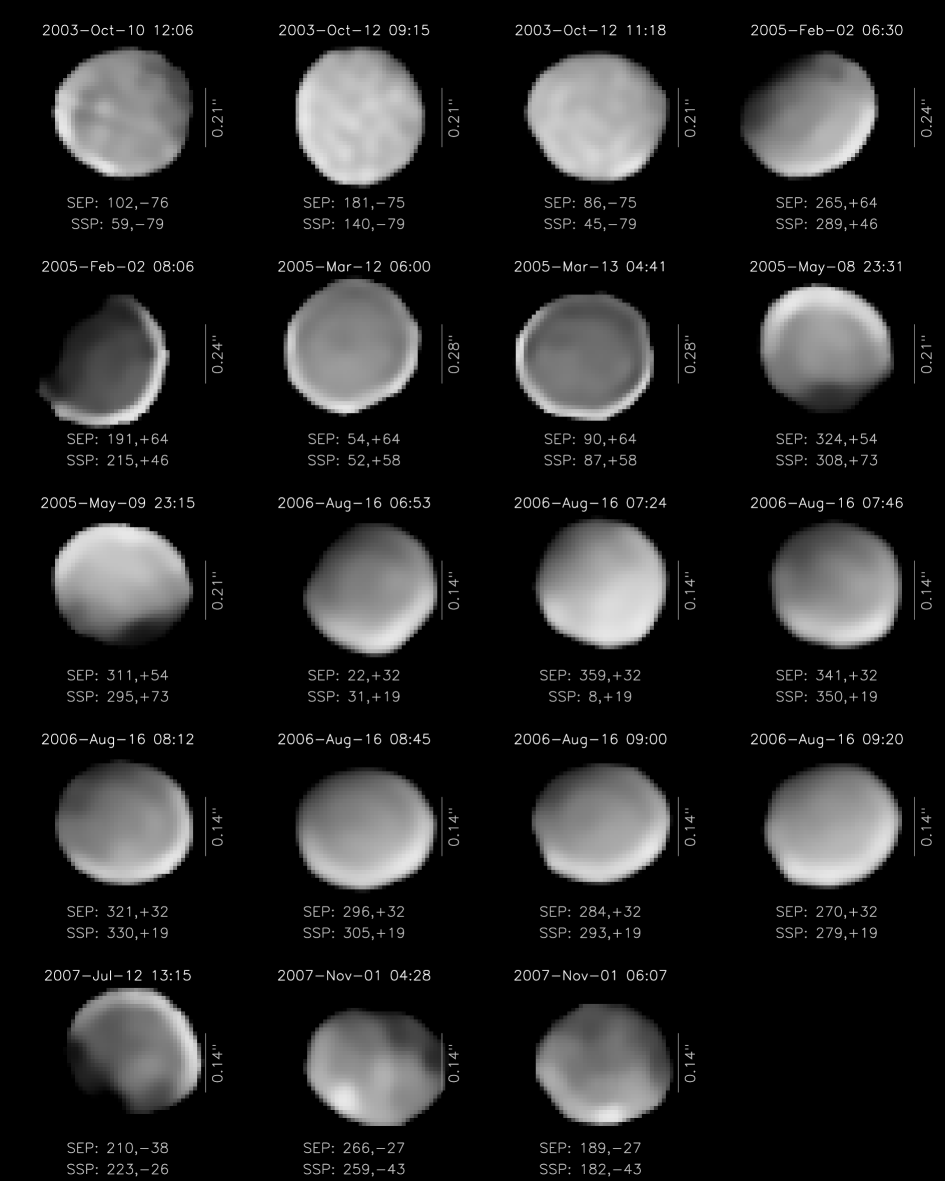
Figure 1: Selected views of (2) Pallas in K-band, oriented to have the rotation axes aligned vertically, with the determined spin vector directed toward the top. The values of the Sub-Earth-Point longitude (SEP_λ), measured positively from 0 to 360 degrees in a right-hand system (following IAU recommendations: Seidelmann et al., 2007), and Sub-Earth-Point latitude (SEP_φ) are indicated under each view. The Sub-Solar-Point (SSP) [longitude, latitude] is also shown. Arbitrary brightness and contrast cuts were applied to highlight the surface features. The edge-brightness ringing present in some images is an artifact (see section 4.2.1) from deconvolution (see Carry et al., 2008, for further explanation). The impact of these artifacts is limited in the current study: it does not influence the shape and we discard the perimeter of the asteroid in each view for the albedo map (see section 5). From these images, the irregular shape of Pallas, as well as important brightness variations across the surface, can be detected easily.

4 Size, shape and spin-vector coordinates

Disk-resolved observations (from space, ground-based AO, radar, or occultations) provide strong constraints on asteroid shape. The limb contour recorded is a direct measurement of the asteroid’s outline on the sky. Combination of such contours leads to the construction of an asteroid shape model and an associated pole solution (Conrad et al., 2007). To improve our shape model, we combined our AO data with the numerous light-curves available for Pallas (51 of them, which led Torppa et al. (2003) to their own shape model).

4.1 Discrimination of the pole solution

Due to an ambiguity inherent in the method and observation geometry, it is sometimes impossible to discriminate between the two possible pole solutions obtained from the light-curve inversion process. Therefore, we produced the two contours of both (light-curve-derived) shape models, as projected onto the plane of the sky for the time of our AO observations, and compared them with our images of Pallas, as shown in Fig. 2. This simple comparison (Cellino et al., 2003; Marchis et al., 2006) allowed us to reject one pole solution (Fig. 2, right) in favor of the other (Fig. 2, left) based on its poor representation of the asteroid contour. Even though the selected pole solution and its associated shape model rendered better the AO images, it was clear that the shape model still needed improvement. Indeed, the light-curve inversion algorithm (Kaasalainen and Torppa, 2001) associates photometric variation with shape and not with albedo. The presence of albedo markings (as found here, see section 5) would thus lead to an erroneous shape. We discuss the development of a new shape model in section 4.2.
Once we had rejected one of the possible pole-solution regions (from light-curves, above), we refined the pole solution by fitting (next section) against our ensemble of AO images. We find the spin-vector coordinates of Pallas to be within 5^∘ of arc of [$\lambda=30$^∘, $\beta=-16$^∘] in the Ecliptic J2000.0 reference frame (Table 4). This value is roughly in agreement with the value (40^∘, -16^∘) in Ecliptic B1950 coordinates [equivalent to (41^∘, -16^∘) in Ecliptic J2000] found by Kryszczyńska et al. (2007) from a synthesis of reported pole solutions (mainly from indirect methods).

Recent pole solutions are reported near our solution. Drummond and Christou (2008) give a solution of (32^∘,-21^∘) $\pm$ 6^∘ (in Ecliptic J2000) based on AO observations done at Lick Observatory. In a follow-up report by the same authors (Drummond et al., 2009), from AO observations at Keck (included as a subset here), a solution of (34^∘,-27^∘) $\pm$ 3^∘ is quoted. These solutions are in rough agreement with the value derived here, and we note that Drummond et al. (2009) list their errors to be model-fit errors only, essentially precisions of the measures, while indicating there may be systematic errors that are not included in the quoted error. Because our solution is derived from a larger number of epochs, and because it also considers extensive light-curve datasets, we think the difference from the solution of Drummond et al. (2009) is the result of systematic errors in their more limited dataset.
The present pole solution implies a high obliquity of $\sim$84^∘, which means seasons on Pallas have high contrast. Large portions of both hemispheres will experience extended periods of constant sunlight or constant darkness over Pallas’ orbital period of 4.6 years. Locations near the poles would remain in total sunlight or darkness for as long as two years.

Pole Solution Selection

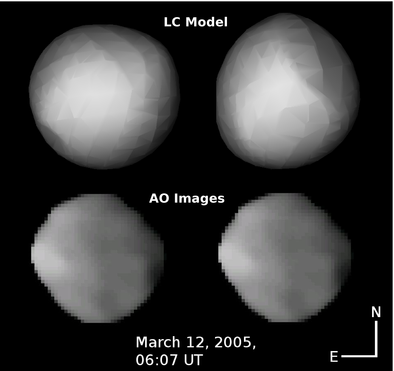
Figure 2: Plane-of-sky synthetic images of the two light-curve shape models compared with AO images for the epoch 2005 Mar 12 UT (in J-band at the VLT). Because the light-curve shape models have no absolute dimensions, their size with respect to the Pallas images is not relevant here and we focus on the overall shape only. The AO images are identical left and right; they are repeated for ease of comparison. This comparison is used only to discriminate between the two pole solutions. Because the shape model on the right, largely asymmetric in this view, does not reproduce correctly the shape of Pallas, we reject it in favor of the other (left) model instead (see text).

Pole solution
$P_{s}$ Ecliptic Equatorial $t_{0}$ $W_{0}$ (h) ($\lambda_{0}$, $\beta_{0}$ in ^∘) ($\alpha_{0}$, $\delta_{0}$ in ^∘) (JD) (^∘) 7.8132214 $\pm$ 0.000002 (30, -16) $\pm$ 5 (33, -3) $\pm$ 5 2433827.77154 38 $\pm$ 2

Table 4: Sidereal period ($P_{s}$, determined from the 51 light-curves) of Pallas and spin-vector coordinates in Ecliptic J2000.0 ($\lambda_{0}$, $\beta_{0}$) and Equatorial J2000.0 ($\alpha_{0}$, $\delta_{0}$) reference frames and the reference epoch $t_{0}$ (see section 4.3). We also report the rotational phase ($W_{0}$) at epoch J2000.0, following IAU guidelines (Seidelmann et al., 2007). The rotational phase $W$ of Pallas at any time is then given by $W=W_{0}+\dot{W}\times d$, where $d$ is the number of days since epoch J2000.0 and $\dot{W}$ is Pallas rotation rate, 1105.8036^∘/day.

4.2 Construction of the shape model

We constructed a shape model, based on both AO observations and optical light-curves, to render the aspect of Pallas at each epoch.

4.2.1 Contour measurement

The deconvolution process is an ill-posed inverse problem (Tikhonov and Arsenine, 1974) and can introduce artifacts in the restored images. Although we carefully cross-checked the images after the deconvolution process, the presence of artifacts was still possible. Because reliable information is provided by limb contours, which are far less subject to artifact contamination in the deconvolution process (see Marchis et al., 2006, Fig. 2), we chose to discard the albedo information from our images at this stage.
We measured 186 limb contours using the Laplacian of a Gaussian wavelet transform (Carry et al., 2008) of the Pallas frames. Then, to minimize introduction of artifacts, we took the median contour (Fig. 3) of each epoch (Table 1) and used them as fiducials during the light-curve inversion. For each observational series, all frames were taken within a span of 4–5 minutes, during which Pallas rotated only about 3–4^∘. This translates into a degradation of the spatial information that is much lower than the highest angular resolution achieved in our images.

Contour extraction

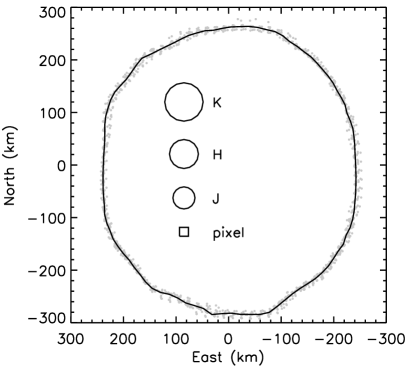
Figure 3: Example of contour extraction for the observations at the epoch 2005 May 8, from the VLT (see Tables 1 & 2), with geometry SEP_λ=307^∘, SEP_β=+54^∘. North is up and east is to the left. Axes are in kilometers (given Pallas’ distance and angular size at observing time). The final contour (dark line) was obtained by taking the median of 13 individual edge measurements (grey spots). One can verify the consistency between each individual contour ($\sigma\sim$13 km). Similar composite contours were created for each epoch listed in Table 1 and used to constrain the shape of Pallas during light-curve inversion (see text). The sizes of the J, H, and K resolution elements, as well as the pixel size, are also shown.

4.2.2 KOALA

The shape and spin model was created by combining the two data modes, photometry (light-curves) and adaptive-optics contours, with the general principle described in Kaasalainen and Lamberg (2006): the joint chi-square is minimized with the condition that the separate chi-squares for the two modes be acceptable (the light-curve fit deviation is 0.019 mag and the profile fit deviation is 0.4 pixel). The light-curve fitting procedure is described in Kaasalainen et al. (2001), and the edge fitting method and the choice of weights for different data modes is described in detail in Kaasalainen [submitted to Inverse Problems and Imaging]. We also used a smoothness constraint (regularizing function) to prevent artificial details in the model, i.e., we chose the simplest model that was capable of fitting successfully the data. Since Pallas is a rather regular body to a first approximation, and the data resolution is limited, we chose to use a function series in spherical harmonics to represent the radii lengths in fixed directions (see Kaasalainen and Torppa, 2001). In addition to reducing the number of free parameters and providing global continuity, the function series, once determined, gives a representation that can be directly evaluated for any number of radii (or any tessellation scheme) chosen without having to carry out the inversion again. The number of function coefficients, rather than the tessellation density, determines the level of resolution.
As discussed in Kaasalainen [submitted to Inverse Problems and Imaging], profile and shadow edges (when several viewing angles are available) contain, in fact, almost as much information on the shape and spin as direct images. In our case, the edges are also considerably more reliable than the information across the deconvolved disk (see section 4.2.1), so the modeling is indeed best done by combining edges, rather than images, with light-curves. The procedure is directly applicable to combining photometry and occultation measurements as well. The technique of combining these three data modes we call KOALA for Knitted Occultation, Adaptive optics, and Light-curve Analysis.

4.3 The irregular shape of Pallas

From the combination of light-curves and high angular-resolution images, we found Pallas to be an irregular asteroid with significant departures from an ellipsoid, as visible in Fig. 1. Our shape model, presented in Fig. 4, is available either on request or from the Internet. Useful parameters (coordinates of the SEP and SSP as well as pole angle) to display the shape model of Pallas, as seen on the plane of the sky at any time, can be computed from the values reported in Table 4 and the following equation from Kaasalainen et al. (2001), which transforms vectors (e.g. Earth-asteroid vector) from the ecliptic reference frame ($\vec{r}_{ecl}$) into the reference frame of the shape model ($\vec{r}_{ast}$).

$$\vec{r}_{ast}=\mathcal{R}_{z}\left(\frac{2\pi}{P_{s}}(t-t_{o})\right)\mathcal{R}_{y}\left(\frac{\pi}{2}-\beta_{0}\right)\mathcal{R}_{z}(\lambda_{0})\vec{r}_{ecl}$$ (1)

where $\lambda_{0}$, $\beta_{0}$ are the pole coordinates in the Ecliptic reference frame, $P_{s}$ the sidereal period (Table 4), $t_{0}$ the epoch of reference (chosen arbitrarily as $t_{0}=2433827.77154$ JD, the starting time of the first light-curve used here), and $t$ is the time. $\mathcal{R}_{i}(\alpha)$ is the rotation matrix representing a rotation by angle $\alpha$ about axis $i$, in the positive sense. Then, we report in Table 5 our best-fit tri-axial ellipsoid values, with measurement dispersion, compared with the Drummond et al. (2009) and Schmidt et al. (2009) studies.

Pallas Shape Model

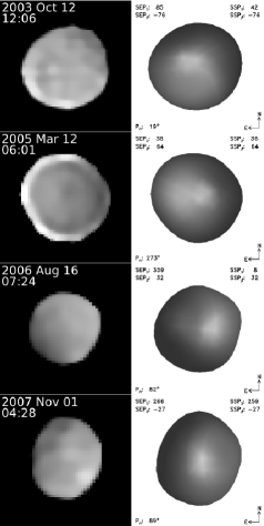
Figure 4: Comparison of the shape model derived in this study (right) with the original frames (left). Sub-Earth-Point (SEP) and Sub-Solar-Point (SSP) coordinates as well as the pole angle $p_{n}$ (defined as the angle in the plane of the sky between the celestial north and the projected asteroid spin-vector, measured counter-clockwise, from north through east) are labeled for each representation of the model. These representations were obtained using the Eproc ephemeris generator (Berthier, 1998). The improvement in the shape model can be seen by comparing the second epoch presented here (2005 Mar 12) with the shape model presented in the upper-left panel of Fig. 2.

Tri-Axial Solution
$a$ $b$ $c$ $R$ $a$/$b$ $b$/$c$ $V$ (km) (km) (km) (km) ($\times 10^{6}$ km³) This work 275 258 238 256 1.06 1.09 70 1 $\sigma$ error 4 3 3 3 0.03 0.03 3 Drummond et al. (2009) 274 252 230 251 1.09 1.10 66 1 $\sigma$ error 2 2 7 3 0.01 0.03 2 Schmidt et al. (2009) 291 278 250 272 1.05 1.11 85 1 $\sigma$ error 9 9 9 9 0.06 0.08 8

Table 5: Best-fit solutions for tri-axial radii ($a$, $b$, $c$) for Pallas. Also given are the mean radius $R=\sqrt[3]{abc}$, axial ratios, and volume ($V$), with their uncertainties for this work, and for two other recent determinations: Keck (Drummond et al., 2009) and HST (Schmidt et al., 2009). For the current study, the dimension uncertainties are derived by scaling the shape model, for each image, to best render the asteroid contour. The dimensions are then determined using the mean values of the scaling factor for the ensemble of images, and the 1 $\sigma$ reported here comes from the standard deviation of the population of scaling factors.

The dimensions derived here for Pallas are somewhat larger, at the few-$\sigma$ level, than those derived by Drummond et al. (2009). The quoted errors by Drummond et al., however, do not include possible systematic effects, which they indicate could be in the range of 1-2% of the values. Once their quoted errors are augmented to include systematics, their dimensions are entirely consistent with our derived values. The smaller error bar quoted here for the $c$ dimension results from more observations, taken over a wider span of SEP latitudes (Table 1). We continue to refine our estimates of our absolute accuracy, but we are confident it is significantly smaller than the difference (16 km) between our value for the mean radius ($R=256\pm 3$ km) and that from HST WFPC2 ($R=272\pm 9$ km) of Schmidt et al. (2009). Our method to determine the error relies on searching for the minimum and maximum possible dimensions of the shape-model contours that would be consistent with the images. Therefore, the quoted errors are the best approximation to absolute accuracy at this time. Further, in search of possible systematics in our technique, we have run a range of simulations for Pallas and a few other asteroids for which we have data. The preliminary results are that the errors quoted here appear to include systematics and, in any case, the absolute errors are unlikely to be much larger than the error quoted here. Two issues that may be relevant to systematics of the HST observations relative to ours, are 1) the WFPC2 PSF, although stable and well characterized, is under-sampled (giving a resolution set by 2 pixels, or about 149 km at all wavebands) and 2) the lack of deconvolution (for size determination), which would naturally result in larger values (see Fig. 3 in Marchis et al., 2006, for instance).
Next, we present in Fig. 5 our shape model, oriented on the sky to correspond to the times of four stellar occultations by Pallas (Dunham and Herald, 2008). To assess quantitatively the match between the shape model from the AO/light-curve observations and the occultation chords, we show in Fig. 6 the radius of the shape model as a function of azimuth angle from the center of the projected figure of the body, along with the measured endpoints of the chords (and their associated uncertainties). The correspondence for the 1985 and 2001 events is quite good, while that for 1978 and 1983 is less so. In Table 6, we display the RMS deviation of the chords from the shape model, both in km and in terms of the occultation uncertainties ($\sigma_{c}$). The 1985 and 2001 events are about 1 $\sigma$, even without making an attempt to modify the shape model. The 3 $\sigma$ for 1983 is still good, considering that this is not a description of a fit of a model to these (occultation) data, but instead assessing how well a model, fit to other data sets, corresponds to the occultation data. The 6 $\sigma$ deviation for 1978 is driven almost entirely by one chord (the RMS deviation without taking this chord into account drops to 1.3 $\sigma$, see Table 6).
Consideration of the RMS deviation in km shows that the observed deviation between the shape model and the occultation chords is on the same scale as possible topographic features. The localized deviations observed may thus reflect the presence of local topography. We found the RMS deviation similar to the uncertainty resulting from the typical occultation-timing error of 0.3 s. Here, we are demonstrating the potential utility of KOALA, by showing rough quantitative agreement between occultation and AO/light-curve-derived shape models. We are showing that the occultations are consistent with our triaxial dimensions as well as the general shape. For future work, we will use the occultation data as additional constraints on the shape model itself, modifying the shape accordingly.
Although the occultations show that the shape model is globally correct, there may exist local topography where no limb measurements were available to constrain the shape. As an exemple, the flat region or facet at the S-E limb in the upper right of Fig. 5 is not borne out by the chords ($\sim$ 20 km mismatch between the model and the occultation chords). This facet appears in the northern hemisphere of Pallas, where a large dark albedo patch is also present (see section 5.2). Because our technique does not yet take into account the albedo information during the inversion, a dark patch may be misrepresented as a deficit/depression if no limb measurement from AO constrains it. This highlights the need for future development of the KOALA technique, including the effects of albedo, and the need for continued acquisition of high-quality imaging at the widest range of geometries (SEP longitude and latitude).

Comparison with occultations

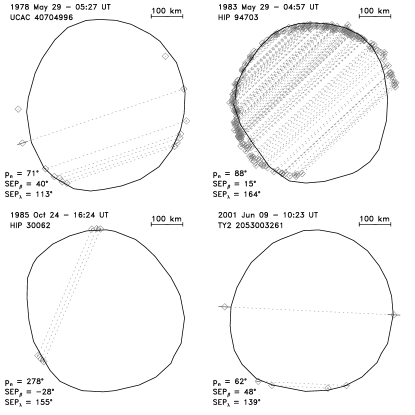
Figure 5: Comparison of our shape model with occultation chords for four occultation events. We use the method described by Berthier (1999) to convert the occultation timings reported by Dunham and Herald (2008) to their print on the plane of the sky. Celestial north is up and east is to the left. For each occultation, we list the date and time (UT), the occulted star, and the SEP coordinates and pole angle $p_{n}$ (defined in Fig. 4) for Pallas. For each chord, the diamonds represent the exact time of disappearance and reappearance as reported by the observer, linked by the dashed lines, and the solid lines represent the error stated by the observer.

Occultation radial profiles

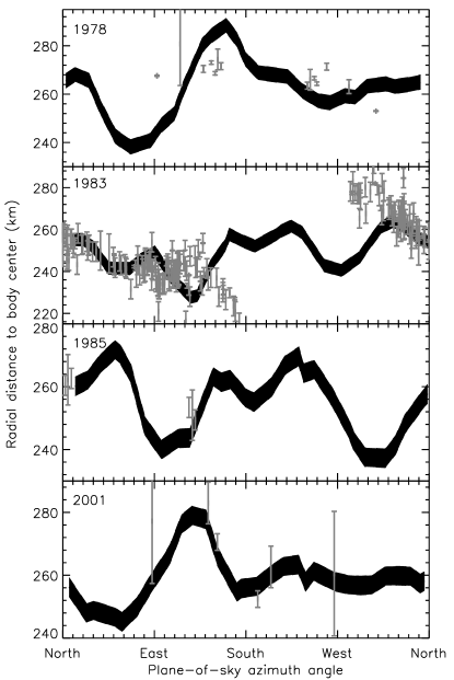
Figure 6: Higher resolution view of the contours for the four occultations presented in Fig. 5. The distance to the body center of the shape model, and the locations of the chord endpoints, are represented as a function of an angle in the plane of sky (measured counter-clockwise from the celestial north through east). The chord endpoints and their associated errors are represented by the grey bars. The black bands show the contour of the shape model with its uncertainty.

Comparison of the Occultations and the Shape Model
Occultation Date Chords $<\sigma_{c}>$ RMS RMS (UT) (#) (km) (km) ($\sigma_{c}$) 1978 May 29 - 05:27 ^α 7 5.4 12.9 6.1 1978 May 29 - 05:27 ^β 6 6.2 6.3 1.3 1983 May 29 - 04:57 130 7.6 9.6 3.7 1985 Oct 24 - 16:24 3 9.6 6.1 0.8 2001 Jun 09 - 10:23 3 19.4 7.5 0.6 $\alpha$ including the KAO chord $\beta$ without the KAO chord, with figure-center readjusted accordingly

Table 6: For each occultation event, we give the RMS deviation of the endpoints of a chord from the shape-model edge (defined as the intersection of the shape-model edge with a line from the body center to the chord endpoint). The values are shown in km and also computed in terms of the uncertainties, $\sigma_{c}$, of the chord endpoints (computed individually for each endpoint, because they vary). Thus, the last column shows how far from the edge the chord endpoints typically lie, in terms of chord uncertainty. The column labeled $<$$\sigma_{c}$$>$ is the average value of the chord uncertainty for that epoch, reported in km. Considering these values are not representing a goodness of fit, because the model is not being adjusted for these values, the deviations are reasonable for all but 1978. For 1978, the RMS deviation is dominated by one chord, from Kuiper Airborne Observatory (KAO), and is improved substantially by removal of this one chord (line labeled $\beta$).

Because of the high inclination of its orbit (35^∘), Pallas remains above or below the canonical asteroid “belt” (and the ecliptic plane) most of the time. As a result, mass determinations for Pallas generally show poor agreement, depending on the method used (see Hilton, 2002, for a review): perturbation of Mars (e.g., Standish and Hellings, 1989), asteroid close encounters (e.g., Goffin, 2001), or ephemeris theory (Fienga et al., 2008). To be conservative, we use the conservative estimate from Michalak (2000), which includes consideration of most previous mass estimates for Pallas. That value is 1.2 $\times$ 10^-10 M_⊙, with an uncertainty of $\pm$ 0.3 $\times$ 10^-10 M_⊙. Combined with our new estimates for Pallas’ dimensions, and hence volume, we derive a density for Pallas of $\rho=3.4\pm$ 0.9 g.cm^-3, where the uncertainty on the mass now dominates the density uncertainty.
Until recently (Schmidt et al., 2009; Drummond et al., 2009), the volume of Pallas was poorly constrained. The IRAS measurement led to a density of $\rho_{\textrm{\tiny{IRAS}}}=3.7\pm 1.1$ g.cm^-3, and not enough occultations were observed to derive an accurate volume (see Drummond and Cocke, 1989). The density derived here agrees with Drummond et al. (2009) at the 5% level, but is about 20% higher than that determined by Schmidt et al. (2009) due to the differences in measured dimensions (see above). Making further improvements on the density determination will now require improved mass estimates.
The difference between the density of (2) Pallas ($3.4\pm$ 0.9 g.cm^-3) and that of (1) Ceres ($\sim$2.2 g.cm^-3, Carry et al., 2008) presents a bit of a puzzle. Because Ceres and Pallas have been predicted to present almost no macro-porosity (Britt et al., 2002), their bulk densities should reflect something close to the mineral density. This difference suggests a compositional mismatch between these two large bodies, even though it has been believed for years that they have a similar composition (e.g., Larson et al., 1983), close to that of carbonaceous chondrites. The orbit of Pallas, however, being more eccentric than that of Ceres, has a perihelion that is closer to the Sun by 0.4 AU than the perihelion of Ceres. Ceres may thus have retained more hydrated (and less dense) materials, as is generally proposed to explain its low density (e.g., see McCord and Sotin, 2005). It is also possible that Ceres may retain reservoirs of water ice and/or may have a somewhat different internal structure than Pallas. For example, the near-surface of Ceres may support extensive voids relative to Pallas, resulting from sublimation of sub-surface water ice, as predicted by the models of its internal structure (Fanale and Salvail, 1989). Marginal detection of sublimation was claimed by A’Hearn and Feldman (1992), although more recent observations (Rousselot et al., 2008) do not support this idea. Based on its near-infrared spectrum, Pallas appears to lack a signature of organic or icy material. (Jones et al., 1990). We suggest that the sum of the evidence points to a dry Pallas, relative to Ceres.

5 Surface mapping

As highlighted in Greeley and Batson (1990), the best way to study planetary landmarks is to produce surface maps. It allows location and comparison of features between independent studies and allows correction of possible artifacts (e.g., from deconvolution). Here we do not describe the whole process of extracting surface maps from AO asteroid images, because it has been covered previously for Ceres (Carry et al., 2008). Instead, we report below the main improvements with respect to our previous study.

5.1 Method

Geometry:

Because a 3-D surface cannot be mapped onto a plane without introducing distortions, the projection choice is crucial, and depends on the geometry of the observations. Due to the high obliquity of Pallas (84^∘) and its inclined orbit (35^∘), the observations presented here span almost the entire latitude range. Following the recommendation of Greeley and Batson (1990), we produced one map for the equatorial band (Equidistant Cylindrical Projection) and two others for the polar regions (Orthographic Projection), thereby minimizing distortion over the entire surface of Pallas. We used the Goldberg and Gott (2006) mapping flexion quantification method to choose both projections for this specific observation geometry.

Region of interest:

We decided to exclude from the maps the outer annulus of the apparent disk of the asteroid in each image. We did this for two reasons: 1) the image scale (km/pixel) and spatial resolution are degraded there (Carry et al., 2008, section 4.2) and 2) the edges of many of the images suffer from brightness-ringing artifacts resulting from deconvolution. We defined a Region Of Interest (ROI) to select the range of pixels to be used for mapping. The ROI was defined by the projected shape of Pallas, reduced to a given percent of its radius to exclude any artifact. We defined the percentage for each night by inspection of the degree of ringing present after image restoration. The resulting ROI percentages are given in Table 2.

Definition of the planetocentric coordinate system:

We define here, for the first time, a planetocentric coordinates system for Pallas, following the guidelines of the IAU Working Group on cartographic coordinates and rotational elements (Seidelmann et al., 2007). Longitudes are measured from 0^∘ to 360^∘, following the right-hand rule with respect to the spin vector. The prime meridian is aligned with the long axis, pointing toward negative $x$ in the shape model reference frame. Latitudes are measured $\pm$90^∘ from the equator, with +90^∘ being in the direction of the spin vector.

Projection:

We used the shape model of Pallas (see section 4.3) to convert image pixels to their prints on the surface of Pallas. For each image, we produced an equivalent image of the shape model projected onto the plane of the sky. We then derived the planetocentric coordinates of each pixel (longitude and latitude). Finally, we convert those planetocentric coordinates to x, y positions on the map, using the translation equations appropriate for the particular map projection.

Combination of images into maps:

There was no overlap between the northern and southern hemispheres in our data. Therefore, we had to arbitrarily set their relative brightness to produce a complete map. Ultimately, we assumed both hemispheres to have the same mean albedo, because no evidence for such a difference exists in the literature. To handle redundant coverage, i.e., where more than one image covers a specific region, we use an average of all the images, with higher weight given to higher resolution and/or higher quality images (see Carry et al., 2008, for detailed explanation).

5.2 (2) Pallas surface in the near-infrared

Because the J and H filters were used only sparsely (Table 1), the K-band map covers a larger fraction of the Pallas surface (80% for K vs. 40% for J and H). So limited imaging can, of course, restrict the explored area on the asteroid surface; but also, fewer overlapping images of one area will result in greater errors than for regions that have a larger number of redundant images.

As explained in section 4.2.1, the deconvolution process can lead to the creation of artifacts. Although we rejected deconvolved images of poor quality and re-applied the Mistral deconvolution process until the dataset was self-consistent, the final products can still show discrepancies between images of the same region of Pallas (e.g., introduced by the incomplete AO correction). The best way to smooth out such artifacts is to combine as many images as possible, and use their mean value to produce the final maps. This method assumes that the probability of recovering real information is greater than the probability of introducing additional artifacts with Mistral. This assumption is increasingly valid with increasing signal-to-noise ratio and increasing number of overlapping images (our observations are optimized to provide high signal-to-noise, usually at levels of several hundred).

An additional test of the validity of the Mistral deconvolution comes from the comparison of AO-VLT deconvolved images of bodies also observed in situ by spacecraft. Ground-based observations of Jupiter’s moon Io (Marchis et al., 2002) and Saturn’s moon Titan (Witasse et al., 2006) have been found to be in good agreement with sizes measured from Galileo and Cassini spacecraft data.

K-band maps

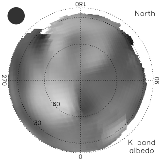
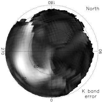
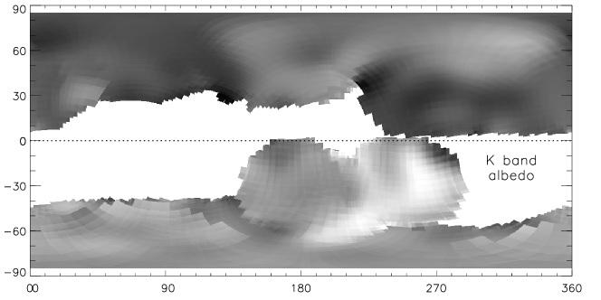
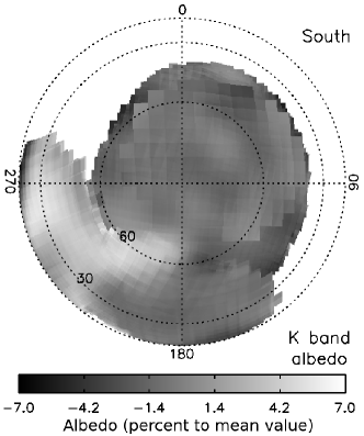
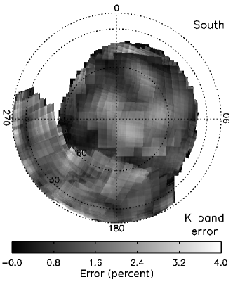
Figure 7: K-band map covering $\sim$80% of Pallas’ surface. The areas in white are terra incognita due to the limited ROI (see text) and Pallas’ spatial orientation during the observations (Table. 1), including most of the equatorial regions. The final estimated resolution element $\Theta$ for this composite map is shown at the upper-left corner. The albedo varies by about $\pm$6% around the mean surface value for each map. We estimate the errors to be limited to 4% maximum. The grey scale is common for the three maps. The mapping for the southern hemisphere in general appears coarser than for the northern hemisphere, due to the smaller number of available images for the southern hemisphere. Any feature or albedo distribution present in these maps has a very low probability of being an artifact.

J- and H-band maps

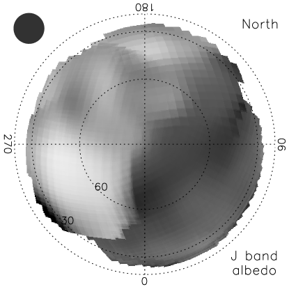
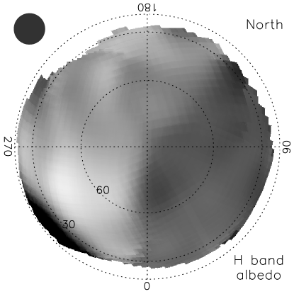
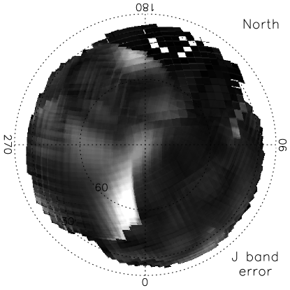
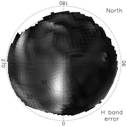
Figure 8: Same as for the K-band observations (Fig. 7). The coarser appearance of these maps results from fewer images being used to produce the maps (27 for J and 44 for H, vs. 115 for K). We only produced an Orthographic projection for these filters because the southern hemisphere was not imaged in these bands. As for the K-band, the albedo variations are within $\pm$6% of the mean surface value for each map and we estimate the errors to be limited to 4% maximum. The final estimated resolution elements for the composites are shown also to the upper left of each map, as in Fig. 7.

The J-, H- and K-band maps shown in Fig. 7 and Fig. 8 are the result of combining 27, 44 and 115 individual projections, respectively. The spatial resolution for these composite maps is nearly equivalent across the three bands, and is $\sim$60 km. The amplitude of the albedo variation is within $\pm$6% of the mean surface value for each band. From the albedo error maps (obtained by measuring, for each pixel, the intensity dispersion among the individual maps), we report a maximal error of $\sim$4% (mean error is below 2.5%).
Pallas shows a large, dark region between 0^∘ and $\sim$120^∘ in longitude in the northern hemisphere, where the shape model presents a facet or “depression”. The fact that we see this feature at all wavelengths suggests that it is real and could be associated with a geological feature such as an impact crater. However, because the light-curve inversion was done without taking into account the albedo information, the depression seen in our model may be an artifact created by the light-curve inversion algorithm (as suggested by the occultation chords, see Fig. 5). In future versions of the KOALA method, we will attempt to use the albedo information from the images to improve the shape model.
Some other features are remarkable, such as the dark spot (diameter $\sim$70 km) surrounded by a bright annulus (about 180 km at its largest extent) at (185^∘, +50^∘) or the bright region (diameter of $\sim$110 km) around (300^∘, +60^∘). Southern features are more difficult to interpret because of the higher noise and the lack of observations in J- and H-band that preclude a cross-check with the features in the K-band observations.
The surface of Pallas appears to have fewer small-scale structures (of size comparable to the resolution element) than Ceres (Li et al., 2006; Carry et al., 2008), even though both objects were observed at approximately the same spatial resolution. Similarly, Vesta also does not exhibit small-scale features when observed at comparable spatial resolution (see Binzel et al., 1997; Li et al., 2008).
To look for color variations, we also selected several regions in the northern hemisphere (three dark and four bright) and measured their relative flux in the three wavebands. As a result, we detect spectral variations slightly above the noise level, but without remarkable behavior. These differences could be due to morphological features or differences in the surface composition and/or regolith properties (such as grain size). One could interpret these variations as minealogical heterogeneity, but the differences are weak with the existing dataset.

6 Conclusion

We report here the first study of an asteroid using a new approach combining light-curves and occultation data with high-angular resolution images obtained with adaptive optics (AO), which we have termed KOALA for Knitted Occultation, Adaptive optics and Light-curve Analysis. This method allows us to derive the spin vector coordinates, and to produce an absolute-sized shape model of the asteroid, providing an improved volume measurement. This method can be used on any body for which light-curves and disk-resolved images are available at several geometries.

Here, we analyze all the near-infrared high-angular resolution images of Pallas that we acquired from 2003 to 2007. We find the spin vector coordinates of Pallas to be within 5^∘ of (30^∘, -16^∘) in the Ecliptic J2000.0 reference frame, indicating a high obliquity of about 84^∘ and implying large seasonal effects on Pallas.
The derived shape model reproduces well both the Pallas’ projected outline on the sky and its light-curve behavior at all epochs. Our best-fit tri-axial ellipsoid radii are $a$=275 $\pm$ 4 km, $b$= 258 $\pm$ 3 km, and $c$= 238 $\pm$ 3 km, allowing us to estimate an average density for Pallas of 3.4 $\pm$ 0.9 g.cm^-3 (using M=(1.2 $\pm$ 0.3) $\times$ 10^-10 M_⊙ from Michalak, 2000). The density uncertainty is now almost entirely due to mass uncertainty. This density might be interpreted as a result of a dryer Pallas with respect to Ceres (supported by spectroscopic studies).

The observation of such a large difference in the bulk density of two large asteroids of similar taxonomic type, of apparently similar surface compositions, and apparently lacking in significant macro-porosity, underscores the need for dedicated programs to monitor close encounters between asteroids (e.g., from GAIA observations, Mouret et al., 2007), in turn allowing us to derive more accurate masses and improve our knowledge of asteroid densities.
We also present the first albedo maps of Pallas, revealing features with diameters in the 70$-$180 km range and an albedo contrast of about 6% with respect to the mean surface albedo. Weak spectral variations are also reported.

References

- A’Hearn and Feldman (1992) M. F. A’Hearn and P. D. Feldman, 1992. Water vaporization on Ceres. Icarus, 98:54–60.
- Berthier (1998) J. Berthier, 1998. Définitions relatives aux éphémérides pour l’observation physique des corps du système solaire. Notes scientifique et techniques du Bureau des longitudes, S061.
- Berthier (1999) J. Berthier, 1999. Principe de réduction des occultations stellaires. Notes scientifique et techniques du Bureau des longitudes, S064.
- Binzel et al. (1997) R. P. Binzel, M. J. Gaffey, P. C. Thomas, B. H. Zellner, A. D. Storrs, and E. N. Wells, 1997. Geologic Mapping of Vesta from 1994 Hubble Space Telescope Images. Icarus, 128:95–103.
- Bottke et al. (2002) W. F. Bottke, Jr., A. Cellino, P. Paolicchi, and R. P. Binzel, 2002. An Overview of the Asteroids: The Asteroids III Perspective. Asteroids III, pages 3–15.
- Britt et al. (2002) D. T. Britt, D. K. Yeomans, K. R. Housen, and G. J. Consolmagno, 2002. Asteroid Density, Porosity, and Structure. Asteroids III, pages 485–500.
- Bus and Binzel (2002) S. J. Bus and R. P. Binzel, 2002. Phase II of the Small Main-Belt Asteroid Spectroscopic Survey: A Feature-Based Taxonomy. Icarus, 158:146–177.
- Carry et al. (2008) B. Carry, C. Dumas, M. Fulchignoni, W. J. Merline, J. Berthier, D. Hestroffer, T. Fusco, and P. Tamblyn, 2008. Near-Infrared Mapping and Physical Properties of the Dwarf-Planet Ceres. Astronomy and Astrophysics, 478(4):235–244.
- Cellino et al. (2003) A. Cellino, E. Diolaiti, R. Ragazzoni, D. Hestroffer, P. Tanga, and A. Ghedina, 2003. Speckle interferometry observations of asteroids at TNG. Icarus, 162:278–284.
- Conrad et al. (2007) A. Conrad, C. Dumas, W. J. Merline, J. D. Drummond, R. D. Campbell, R. W. Goodrich, D. Le Mignant, F. H. Chaffee, T. Fusco, S. H. Kwok, and R. I. Knight, 2007. Direct measurement of the size, shape, and pole of 511 Davida with Keck AO in a single night. Icarus, 191(2):616–627.
- Davis (1999) D. R. Davis, 1999. The Collisional History of Asteroid 253 Mathilde. Icarus, 140:49–52.
- Descamps et al. (2008) P. Descamps, F. Marchis, J. Pollock, J. Berthier, F. Vachier, M. Birlan, M. Kaasalainen, A. W. Harris, M. H. Wong, W. J. Romanishin, E. M. Cooper, K. A. Kettner, P. Wiggins, A. Kryszczynska, M. Polinska, J.-F. Coliac, A. Devyatkin, I. Verestchagina, and D. Gorshanov, 2008. New determination of the size and bulk density of the binary Asteroid 22 Kalliope from observations of mutual eclipses. Icarus, 196:578–600.
- Drummond and Christou (2008) J. D. Drummond and J. C. Christou, 2008. Triaxial ellipsoid dimensions and rotational poles of seven asteroids from Lick Observatory adaptive optics images, and of Ceres. Icarus, 197:480–496.
- Drummond et al. (2009) J. D. Drummond, J. C. Christou, and J. Nelson, 2009. Triaxial ellipsoid dimensions and poles of asteroids from AO observations at the Keck-II telescope. Icarus. doi:10.1016/j.icarus.2009.02.011.
- Drummond and Cocke (1989) J. D. Drummond and W. J. Cocke, 1989. Triaxial ellipsoid dimensions and rotational pole of 2 Pallas from two stellar occultations. Icarus, 78:323–329.
- Dunham et al. (1990) D. W. Dunham, J. B. Dunham, R. P. Binzel, D. S. Evans, M. Freuh, G. W. Henry, M. F. A’Hearn, R. G. Schnurr, R. Betts, H. Haynes, R. Orcutt, E. Bowell, L. H. Wasserman, R. A. Nye, H. L. Giclas, C. R. Chapman, R. D. Dietz, C. Moncivais, W. T. Douglas, D. C. Parker, J. D. Beish, J. O. Martin, D. R. Monger, W. B. Hubbard, H. J. Reitsema, A. R. Klemola, P. D. Lee, B. R. McNamara, P. D. Maley, P. Manly, N. L. Markworth, R. Nolthenius, T. D. Oswalt, J. A. Smith, E. F. Strother, H. R. Povenmire, R. D. Purrington, C. Trenary, G. H. Schneider, W. J. Schuster, M. A. Moreno, J. Guichard, G. R. Sanchez, G. E. Taylor, A. R. Upgren, and T. C. von Flandern, 1990. The size and shape of (2) Pallas from the 1983 occultation of 1 Vulpeculae. Astronomical Journal, 99:1636–1662.
- Dunham and Herald (2008) D. W. Dunham and D. Herald. Asteroid Occultations V6.0. EAR-A-3-RDR-OCCULTATIONS-V6.0. NASA Planetary Data System, 2008.
- Fanale and Salvail (1989) F. P. Fanale and J. R. Salvail, 1989. The water regime of asteroid (1) Ceres. Icarus, 82:97–110.
- Fienga et al. (2008) A. Fienga, H. Manche, J. Laskar, and M. Gastineau, 2008. INPOP06: a new numerical planetary ephemeris. Astronomy and Astrophysics, 477(1):315–327.
- Fujiwara et al. (2006) A. Fujiwara, J. Kawaguchi, D. K. Yeomans, M. Abe, T. Mukai, T. Okada, J. Saito, H. Yano, M. Yoshikawa, D. J. Scheeres, O. S. Barnouin-Jha, A. F. Cheng, H. Demura, G. W. Gaskell, N. Hirata, H. Ikeda, T. Kominato, H. Miyamoto, R. Nakamura, S. Sasaki, and K. Uesugi, 2006. The Rubble-Pile Asteroid Itokawa as Observed by Hayabusa. Science, 312:1330–1334.
- Fusco (2000) T. Fusco. Correction Partielle Et Anisoplanétisme En Optique. PhD thesis, Université de Nice Sophia-Antipolis, 2000.
- Goffin (2001) E. Goffin, 2001. New determination of the mass of Pallas. Astronomy and Astrophysics, 365:627–630.
- Goldberg and Gott (2006) D. M. Goldberg and J. R. I. Gott, 2006. Flexion and Skewness in Map Projections of the Earth. ArXiv Astrophysics e-prints.
- Greeley and Batson (1990) R. Greeley and R. M. Batson. Planetary Mapping. Cambridge University Press, 1990.
- Hilton (2002) J. L. Hilton, 2002. Asteroid Masses and Densities. Asteroids III, pages 103–112.
- Jones et al. (1990) T. D. Jones, L. A. Lebofsky, J. S. Lewis, and M. S. Marley, 1990. The composition and Origin of the C,P and D Asteroids: Water as Tracer of Thermal Evolution in the Outer Belt. Icarus, 88:172–193.
- Kaasalainen and Lamberg (2006) M. Kaasalainen and L. Lamberg, 2006. Inverse problems of generalized projection operators. Inverse Problems, 22:749–769.
- Kaasalainen et al. (2002) M. Kaasalainen, S. Mottola, and M. Fulchignoni, 2002. Asteroid Models from Disk-integrated Data. Asteroids III, pages 139–150.
- Kaasalainen and Torppa (2001) M. Kaasalainen and J. Torppa, 2001. Optimization Methods for Asteroid Lightcurve Inversion - I. Shape Determination. Icarus, 153:24–36.
- Kaasalainen et al. (2001) M. Kaasalainen, J. Torppa, and K. Muinonen, 2001. Optimization Methods for Asteroid Lightcurve Inversion - II. The Complete Inverse Problem. Icarus, 153:37–51.
- Kryszczyńska et al. (2007) A. Kryszczyńska, A. La Spina, P. Paolicchi, A. W. Harris, S. Breiter, and P. Pravec, 2007. New findings on asteroid spin-vector distributions. Icarus, 192:223–237.
- Larson et al. (1983) H. P. Larson, M. A. Feierberg, and L. A. Lebofsky, 1983. The Composition of Asteroid 2 Pallas and Its Relation to Primitive Meteorites. Icarus, 56:398–408.
- Lenzen et al. (2003) R. Lenzen, M. Hartung, W. Brandner, G. Finger, N. N. Hubin, F. Lacombe, A.-M. Lagrange, M. D. Lehnert, A. F. M. Moorwood, and D. Mouillet, 2003. NAOS-CONICA first on sky results in a variety of observing modes. SPIE, 4841:944–952.
- Li et al. (2006) J.-Y. Li, L. A. McFadden, J. W. Parker, E. F. Young, S. A. Stern, P. C. Thomas, C. T. Russell, and M. V. Sykes, 2006. Photometric analysis of 1 Ceres and surface mapping from HST observations. Icarus, 182:143–160.
- Li et al. (2008) J.-Y. Li, L. A. McFadden, P. C. Thomas, M. J. Mutchler, J. W. Parker, E. F. Young, C. T. Russell, M. V. Sykes, and B. Schmidt, 2008. Photometric mapping of Vesta from HST observations. ACM Meeting. Poster 8288.
- Marchis et al. (2002) F. Marchis, I. de Pater, A. G. Davies, H. G. Roe, T. Fusco, D. Le Mignant, P. Descamps, B. A. Macintosh, and R. Prangé, 2002. High-Resolution Keck Adaptive Optics Imaging of Violent Volcanic Activity on Io. Icarus, 160:124–131.
- Marchis et al. (2006) F. Marchis, M. Kaasalainen, E. F. Y. Hom, J. Berthier, J. Enriquez, D. Hestroffer, D. Le Mignant, and I. de Pater, 2006. Shape, size and multiplicity of main-belt asteroids. Icarus, 185(1):39–63.
- McCord and Sotin (2005) T. B. McCord and C. Sotin, 2005. Ceres: Evolution and current state. Journal of Geophysical Research (Planets), 110:5009–5023.
- Merline et al. (2002) W. J. Merline, S. J. Weidenschilling, D. D. Durda, J.-L. Margot, P. Pravec, and A. D. Storrs, 2002. Asteroids Do Have Satellites. Asteroids III, pages 289–312.
- Michalak (2000) G. Michalak, 2000. Determination of asteroid masses — I. (1) Ceres, (2) Pallas and (4) Vesta. Astronomy and Astrophysics, 360:363–374.
- Millis and Dunham (1989) R. L. Millis and D. W. Dunham, 1989. Precise measurement of asteroid sizes and shapes from occultations. Asteroids II, pages 148–170.
- Mouret et al. (2007) S. Mouret, D. Hestroffer, and F. Mignard, 2007. Asteroid masses and improvement with GAIA. Astronomy and Astrophysics, 472:1017–1027.
- Mousis et al. (2008) O. Mousis, Y. Alibert, D. Hestroffer, U. Marboeuf, C. Dumas, B. Carry, J. Horner, and F. Selsis, 2008. Origin of volatiles in the main belt. Monthly Notices of the Royal Astronomical Society, 383:1269–1280.
- Mugnier et al. (2004) L. M. Mugnier, T. Fusco, and J.-M. Conan, 2004. MISTRAL: a Myopic Edge-Preserving Image Restoration Method, with Application to Astronomical Adaptive-Optics-Corrected Long-Exposure Images. Journal of the Optical Society of America A, 21(10):1841–1854.
- Rousselot et al. (2008) P. Rousselot, O. Mousis, C. Dumas, E. Jehin, J. Manfroid, B. Carry, and J.-M. Zucconi, 2008. A Search for Escaping Water from Ceres’ Poles. LPI Contributions, 1405:8337.
- Rousset et al. (2003) G. Rousset, F. Lacombe, P. Puget, N. N. Hubin, E. Gendron, T. Fusco, R. Arsenault, J. Charton, P. Feautrier, P. Gigan, P. Y. Kern, A.-M. Lagrange, P.-Y. Madec, D. Mouillet, D. Rabaud, P. Rabou, E. Stadler, and G. Zins, 2003. NAOS, the first AO system of the VLT: on-sky performance. SPIE, 4839:140–149.
- Saint-Pé et al. (1993a) O. Saint-Pé, M. Combes, and F. Rigaut, 1993a. Ceres surface properties by high-resolution imaging from earth. Icarus, 105:271–281.
- Saint-Pé et al. (1993b) O. Saint-Pé, M. Combes, F. Rigaut, M. Tomasko, and M. Fulchignoni, 1993b. Demonstration of adaptive optics for resolved imagery of solar system objects - Preliminary results on Pallas and Titan. Icarus, 105:263–270.
- Schmidt et al. (2009) B. E. Schmidt, P. C. Thomas, J. M. Bauer, J.-Y. Li, S. C. Radcliffe, L. A. McFadden, M. J. Mutchler, J. W. Parker, A. S. Rivkin, C. T. Russell, and S. A. Stern. The 3D Figure and Surface of Pallas from HST. In Lunar and Planetary Institute Science Conference Abstracts, volume 40 of Lunar and Planetary Institute Science Conference Abstracts, pages 2421–2422, 2009.
- Scott (2007) E. R. D. Scott, 2007. Chondrites and the Protoplanetary Disk. Annual Review of Earth and Planetary Sciences, 35:577–620.
- Seidelmann et al. (2007) P. K. Seidelmann, B. A. Archinal, M. F. A’Hearn, A. Conrad, G. J. Consolmagno, D. Hestroffer, J. L. Hilton, G. A. Krasinsky, G. Neumann, J. Oberst, P. Stooke, E. F. Tedesco, D. J. Tholen, P. C. Thomas, and I. P. Williams, 2007. Report of the IAU/IAG Working Group on cartographic coordinates and rotational elements: 2006. Celestial Mechanics and Dynamical Astronomy, 98:155–180.
- Standish and Hellings (1989) E. M. Standish and R. W. Hellings, 1989. A determination of the masses of Ceres, Pallas, and Vesta from their perturbations upon the orbit of Mars. Icarus, 80:326–333.
- Taylor et al. (2007) P. A. Taylor, J.-L. Margot, D. Vokrouhlický, D. J. Scheeres, P. Pravec, S. C. Lowry, A. Fitzsimmons, M. C. Nolan, S. J. Ostro, L. A. M. Benner, J. D. Giorgini, and C. Magri, 2007. Spin Rate of Asteroid (54509) 2000 PH5 Increasing Due to the YORP Effect. Science, 316:274–277.
- Thomas et al. (2005) P. C. Thomas, J. W. Parker, L. A. McFadden, C. T. Russell, S. A. Stern, M. V. Sykes, and E. F. Young, 2005. Differentiation of the asteroid Ceres as revealed by its shape. Nature, 437:224–226.
- Tikhonov and Arsenine (1974) A. N. Tikhonov and V. Arsenine. Méthode de Résolution de Problèmes mal posés. Mir:Moscou, 1974.
- Torppa et al. (2003) J. Torppa, M. Kaasalainen, T. Michalowski, T. Kwiatkowski, A. Kryszczyńska, P. Denchev, and R. Kowalski, 2003. Shapes and rotational properties of thirty asteroids from photometric data. Icarus, 164:346–383.
- van Dam et al. (2004) M. A. van Dam, D. Le Mignant, and B. Macintosh, 2004. Performance of the Keck Observatory adaptive-optics system. Applied Optics, 43(23):5458–5467.
- Veverka et al. (1999) J. Veverka, P. C. Thomas, A. Harch, B. E. Clark, B. Carcich, J. Joseph, S. L. Murchie, N. Izenberg, C. R. Chapman, W. J. Merline, M. Malin, L. A. McFadden, and M. Robinson, 1999. NEAR Encounter with Asteroid 253 Mathilde: Overview. Icarus, 140:3–16.
- Wasserman et al. (1979) L. H. Wasserman, R. L. Millis, O. G. Franz, E. Bowell, N. M. White, H. L. Giclas, L. J. Martin, J. L. Elliot, E. Dunham, D. Mink, R. Baron, R. K. Honeycutt, A. A. Henden, J. E. Kephart, M. F. A’Hearn, H. J. Reitsema, R. Radick, and G. E. Taylor, 1979. The diameter of Pallas from its occultation of SAO 85009. Astronomical Journal, 84:259–268.
- Witasse et al. (2006) O. Witasse, J.-P. Lebreton, M. K. Bird, R. Dutta-Roy, W. M. Folkner, R. A. Preston, S. W. Asmar, L. I. Gurvits, S. V. Pogrebenko, I. M. Avruch, R. M. Campbell, H. E. Bignall, M. A. Garrett, H. J. van Langevelde, S. M. Parsley, C. Reynolds, A. Szomoru, J. E. Reynolds, C. J. Phillips, R. J. Sault, A. K. Tzioumis, F. Ghigo, G. Langston, W. Brisken, J. D. Romney, A. Mujunen, J. Ritakari, S. J. Tingay, R. G. Dodson, C. G. M. van’t Klooster, T. Blancquaert, A. Coustenis, E. Gendron, B. Sicardy, M. Hirtzig, D. Luz, A. Negrao, T. Kostiuk, T. A. Livengood, M. Hartung, I. de Pater, M. Ádámkovics, R. D. Lorenz, H. Roe, E. L. Schaller, M. E. Brown, A. H. Bouchez, C. A. Trujillo, B. J. Buratti, L. Caillault, T. Magin, A. Bourdon, and C. Laux, 2006. Overview of the coordinated ground-based observations of Titan during the Huygens mission. Journal of Geophysical Research (Planets), 111:7–19.