Enhanced Intelligent Driver Model to Access the Impact of Driving Strategies on Traffic Capacity

Abstract

adaptive cruise control, human driving behaviour, car-following model, microscopic traffic simulation, free-flow capacity, dynamic capacity With an increasing number of vehicles equipped with adaptive cruise control (ACC), the impact of such vehicles on the collective dynamics of traffic flow becomes relevant. By means of simulation, we investigate the influence of variable percentages of ACC vehicles on traffic flow characteristics. For simulating the ACC vehicles, we propose a new car-following model that also serves as basis of an ACC implementation in real cars. The model is based on the Intelligent Driver Model [Treiber et al., Physical Review E 62, 1805 (2000)] and inherits its intuitive behavioural parameters: desired velocity, acceleration, comfortable deceleration, and desired minimum time headway. It eliminates, however, the sometimes unrealistic behaviour of the Intelligent Driver Model in cut-in situations with ensuing small gaps that regularly are caused by lane changes of other vehicles in dense or congested traffic. We simulate the influence of different ACC strategies on the maximum capacity before breakdown, and the (dynamic) bottleneck capacity after breakdown. With a suitable strategy, we find sensitivities of the order of 0.3, i.e., 1% more ACC vehicles will lead to an increase of the capacities by about 0.3%. This sensitivity multiplies when considering travel times at actual breakdowns.

1 Introduction

Efficient transportation systems are essential to the functioning and prosperity of modern, industrialized societies. Engineers are therefore seeking solutions to the questions of how the capacity of the road network could be used more efficiently and how operations can be improved by way of intelligent transportation systems (ITS). Achieving this efficiency through automated vehicle control is the long-standing vision in transport telematics. With the recent advent of advanced driver assistance systems, at least partly automated driving is already available for basic driving tasks such as accelerating and braking by means of adaptive cruise control (ACC) systems. An ACC system extends earlier cruise control to situations with significant traffic in which driving at constant speed is not possible. The driver cannot only adjust the desired velocity but also set a certain safe time gap determining the distance to the leading car when following slower vehicles.

Although originally developed to delineate human driving behaviour, car-following models can also be used to describe ACC systems: A radar sensor tracks the car ahead to measure the net distance (gap) and the approaching rate, which serve (besides the own speed) as input quantities just as in many time-continuous car-following models. Then, the ACC system calculates the appropriate acceleration for adapting the speed and the safety gap to the leader. This analogy is scientifically interesting because a ‘good’ car-following model could serve as basis of a control algorithm of a real-world ACC system. On the one hand, the in-vehicle implementation would allow to judge the realism of the considered car-following model which is a further (and promising) approach towards benchmarking the plethora of car-following models. This question has recently been considered with different methods in the literature [Brockfeld et al., 2004; Ossen & Hoogendoorn, 2005; Punzo & Simonelli, 2005; Panwai & Dia, 2005; Kesting & Treiber, 2008a]. On the other hand, from the direct driving experience one may expect new insights for the (better) description of human drivers through adequate follow-the-leader models, which is still an ongoing challenge in traffic science [Treiber et al., 2006; Ossen et al., 2007; Kerner, 2004; Helbing, 2001].

Furthermore, one may raise the interesting question how the collective traffic dynamics will be influenced in the future by an increasing number of vehicles equipped with ACC systems. Microscopic traffic simulations are the appropriate methodology for this since this approach allows to treat ‘vehicle-driver units’ individually and in interaction. The results, however, may significantly depend on the chosen modelling assumptions. In the literature, positive as well as negative effects of ACC systems have been reported [van Arem et al., 2006; Kesting et al., 2008; Davis, 2004; VanderWerf et al., 2002; Marsden et al., 2001]. This puzzling fact points to the difficulty when investigating mixed traffic consisting of human drivers and automatically controlled vehicles: How to describe human and automated driving and their interaction appropriately?

The Intelligent Driver Model (IDM) [Treiber et al., 2000] appears to be a good basis for the development of an ACC system. The IDM shows a crash-free collective dynamics, exhibits controllable stability properties [Helbing et al., 2009], and implements an intelligent braking strategy with smooth transitions between acceleration and deceleration behaviour. Moreover, it has only six parameters with a concrete meaning which makes them measurable. However, the IDM was originally developed as a simple car-following model for one-lane situations. Due to lane changes (‘cut-in’ manoeuvres), the input quantities change in a non-continuous way, in which the new distance to the leader can drop significantly below the current equilibrium distance, particularly if there is dense or congested traffic, the lane change is mandatory, or if drivers have different conceptions of safe distance. This may lead to strong braking manoeuvres of the IDM, which would not be acceptable (nor possible) in a real-world ACC system.

In this paper, we therefore extend the IDM by a new constant-acceleration heuristic, which implements a more relaxed reaction to cut-in manoeuvres without loosing the mandatory model property of being essentially crash-free. This model extension has already been implemented (with some further confidential extensions) in real test cars [Kranke & Poppe, 2008; Kranke et al., 2006]. In a second part of this contribution we apply the enhanced IDM to multi-lane traffic simulations in which we study the collective dynamics of mixed traffic flows consisting of human drivers and adaptive cruise control systems. The vehicles equipped with ACC systems implement a recently proposed traffic-adaptive driving strategy [Kesting et al., 2008], which is realized by a situation-dependent parameter setting for each vehicle.

Our paper is structured as follows: In §2, we will present an improved heuristic of the IDM particularly suited for multi-lane simulations. Section §3 presents traffic-adaptive driving strategies for adaptive cruise control systems. The impact of temporarily changed model parameters on the relevant traffic capacities in heterogeneous traffic flows will be systematically evaluated by simulations in §4. Finally, we will conclude with a discussion in §5.

2 A Model for ACC Vehicles

In this section, we will develop the model equations of the enhanced Intelligent Driver Model. To this, we will first present the relevant aspects of the original Intelligent Driver Model (IDM) [Treiber et al., 2000] in §2 (2.1). While, in most situations, the IDM describes accelerations and decelerations in a satisfactory way, it can lead to unrealistic driving behaviour if the actual vehicle gap is significantly lower than the desired gap, and, simultaneously, the situation can be considered as only mildly critical.

Therefore, in §2 (2.2), we develop an upper limit of a safe acceleration based on the more optimistic ‘constant-acceleration heuristic’ (CAH), in which drivers assume that the leading vehicle will not change its acceleration for the next few seconds. This ansatz is applicable precisely in these situations where the IDM reacts too strongly. In §2 (2.3), we combine the IDM and CAH accelerations to specify the acceleration function of the final model for ACC vehicles (‘ACC model’) such that the well-tested IDM is applied whenever it leads to a plausible behaviour, using the difference $a_{\text{CAH}}-a_{\text{IDM}}$ as an indicator for plausibility. Finally, the properties of the new model are tested by computer simulations in §2 (2.4).

2.1 Intelligent Driver Model

The IDM acceleration is a continuous function incorporating different driving modes for all velocities in freeway traffic as well as city traffic. Besides the (bumper-to-bumper-) distance $s$ to the leading vehicle and the actual speed $v$, the IDM also takes into account the velocity difference (approaching rate) $\Delta v=v-v_{\text{l}}$ to the leading vehicle. The IDM acceleration function is given by

$$a_{\text{IDM}}(s,v,\Delta v) = \frac{\text{d}v}{\text{d}t}=a\left[1-\left(\frac{v}{v_{0}}\right)^{\delta}-\left(\frac{s^{*}(v,\Delta v)}{s}\right)^{2}\,\right],$$ (1)

$$s^{*}(v,\Delta v) = s_{0}+vT+\frac{v\Delta v}{2\sqrt{ab}}.$$ (2)

This expression combines the free-road acceleration strategy $\dot{v}_{\text{free}}(v)=a[1-(v/v_{0})^{\delta}]$ with a deceleration strategy $\dot{v}_{\text{brake}}(s,v,\Delta v)=-a(s^{*}/s)^{2}$ that becomes relevant when the gap to the leading vehicle is not significantly larger than the effective ‘desired (safe) gap’ $s^{*}(v,\Delta v)$. The free acceleration is characterized by the desired speed $v_{0}$, the maximum acceleration $a$, and the exponent $\delta$ characterizing how the acceleration decreases with velocity ($\delta=1$ corresponds to a linear decrease while $\delta\to\infty$ denotes a constant acceleration). The effective minimum gap $s^{*}$ is composed of the minimum distance $s_{0}$ (which is relevant for low velocities only), the velocity dependent distance $vT$ which corresponds to following the leading vehicle with a constant desired time gap $T$, and a dynamic contribution which is only active in non-stationary traffic corresponding to situations in which $\Delta v\neq 0$. This latter contribution implements an ‘intelligent’ driving behaviour that, in normal situations, limits braking decelerations to the comfortable deceleration $b$. In critical situations, however, the IDM deceleration becomes significantly higher, making the IDM collision-free [Treiber et al., 2000]. The IDM parameters $v_{0}$, $T$, $s_{0}$, $a$ and $b$ (see table 1) have a reasonable interpretation, are known to be relevant, are empirically measurable, and have realistic values [Kesting & Treiber, 2008a].

Table 1: Model Parameters

Parameters of the Intelligent Driver Model and the ACC model used in the simulations of §2 (4). The first six parameters are common for both models. The last parameter is applicable to the ACC model only. Parameter Car Truck Desired speed $v_{0}$ 120 km/h 85 km/h Free acceleration exponent $\delta$ 4 4 Desired time gap $T$ 1.5 s 2.0 s Jam distance $s_{0}$ 2.0 m 4.0 m Maximum acceleration $a$ 1.4 m/s² 0.7 m/s² Desired deceleration $b$ 2.0 m/s² 2.0 m/s² Coolness factor $c$ 0.99 0.99

2.2 Constant-Acceleration Heuristic

The braking term of the IDM is developed such that accidents are avoided even in the worst case, where the driver of the leading vehicle suddenly brakes with the maximum possible deceleration $b_{\text{max}}\gg b$ to a complete standstill. Since the IDM does not include explicit reaction times, it is even safe when the time headway parameter $T$ is set to zero.

However, there are situations, characterized by comparatively low velocity differences and gaps that are significantly smaller than the desired gaps, where this worst-case heuristic leads to overreactions. In fact, human drivers simply rely on the fact that the drivers of preceding vehicles will not suddenly initiate full-stop emergency brakings without any reason and, therefore, consider such situations only as mildly critical. Normally this judgement is correct. Otherwise, the frequent observations of accident-free driving at time headways significantly below 1 s, i.e., below the reaction time of even an attentive driver, would not be observed so frequently [Treiber et al., 2006].

In order to characterize this more optimistic view of the drivers, let us investigate the implications of the constant-acceleration heuristic (CAH) on the safe acceleration. The CAH is based on the following assumptions:

• The accelerations of the considered and leading vehicle will not change in the relevant future (generally, a few seconds).

• No safe time headway or minimum distance is required at any moment.

• Drivers react without delay (zero reaction time).

When calculating the maximum acceleration for which the situation remains crash-free, one needs to distinguish whether the velocity of the leading vehicle is zero or nonzero at the time where the minimum gap (i.e., $s=0$) is reached. For given actual values of the gap $s$, velocity $v$, velocity $v_{l}$ of the leading vehicle, and its acceleration $a_{l}$, the maximum acceleration $a_{\text{CAH}}$ leading to no crashes is given by

$$a_{\text{CAH}}(s,v,v_{l},a_{l})=\left\{\begin{array}[]{ll}\frac{v^{2}\tilde{a}_{l}}{v_{l}^{2}-2s\tilde{a}_{l}}&\text{if}\ \ v_{l}(v-v_{l})\leq-2s\tilde{a}_{l},\\ \tilde{a}_{l}-\frac{(v-v_{l})^{2}\Theta(v-v_{l})}{2s}&\text{otherwise,}\end{array}\right.$$ (3)

where the effective acceleration $\tilde{a}_{l}=\min(a_{l},a)$ has been used to avoid artefacts that may be caused by leading vehicles with higher acceleration capabilities. The condition $v_{l}(v-v_{l})=v_{l}\Delta v\leq-2sa_{l}$ is true if the vehicles have stopped at the time the minimum gap $s=0$ is reached. Otherwise, negative approaching rates do not make sense to the CAH and are therefore eliminated by the Heaviside step function $\Theta$.

In figure 1(b), the CAH acceleration (3) has been plotted for a leading vehicle driving at constant velocity. A comparison with figure 1(a) clearly shows that, for small values of the gap $s$, the CAH acceleration is significantly higher (i.e., less negative) than that for the IDM.

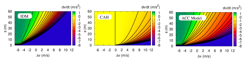
Figure 1: Acceleration functions of (a) the IDM, (b) resulting from the CAH heuristic, (c) of the proposed ACC model as a function of the gap $s$ and the velocity difference (approaching rate) $\Delta v$ to the leading vehicle. The velocity of the leading vehicle and its acceleration $a_{l}$ are given by $v_{l}=20\,\mathrm{m/s}$ and $a_{l}=0$, respectively.

2.3 The ACC Model

For the situations where the IDM leads to unnecessarily strong braking reactions, the CAH acceleration is significantly higher, corresponding to a more relaxed reaction. This heuristic, however, fails on the other side and therefore is not suited to directly model the accelerations of ACC vehicles. Specifically, the CAH leads to zero deceleration for some cases that clearly require at least a moderate braking reaction. This includes a stationary car-following situation ($\Delta v=0$, $a_{\text{l}}=0$), where $a_{\text{CAH}}=0$ for arbitrary values of the gap $s$ and velocity $v$, see figure 1(b). Moreover, since the CAH does not include minimum time headways or an acceleration to a desired velocity, it does not result in a complete model.

For the actual formulation of a model for ACC vehicles, we will therefore use the CAH only as an indicator to determine whether the IDM will lead to unrealistically high decelerations, or not. Specifically, the proposed ACC model is based on following assumptions:

• The ACC acceleration is never lower than that of the IDM. This is motivated by the circumstance that the IDM will lead to crash-free vehicle trajectories for all simulated situations.

• If both, the IDM and the CAH, produce the same acceleration, the ACC acceleration is the same as well.

• If the IDM produces extreme decelerations, while the CAH yields accelerations greater than $-b$, the situation is considered as mildly critical and the ACC acceleration is essentially equal to the comfortable deceleration plus a small fraction $1-c$ of the IDM deceleration.

• If both the IDM and the CAH result in accelerations significantly below $-b$, the situation is seriously critical and the ACC acceleration must not be higher than the maximum of the IDM and CAH accelerations.

• The ACC acceleration should be a continuous and differentiable function of the IDM and CAH accelerations.

Probably the most simple functional form satisfying these criteria is given by (cf. figure 2)

$$a_{\text{ACC}}=\left\{\begin{array}[]{ll}a_{\text{IDM}}&a_{\text{IDM}}\geq a_{\text{CAH}},\\ (1-c)\,a_{\text{IDM}}+c\left[a_{\text{CAH}}+b\tanh\left(\frac{a_{\text{IDM}}-a_{\text{CAH}}}{b}\right)\right]&\text{otherwise.}\end{array}\right.$$ (4)

This acceleration equation of the ACC model is the main model-related result of this paper. Figure 1 shows that the conditions listed above are fulfilled. Notably, the ACC model leads to more relaxed reactions in situations in which the IDM behaves too conservatively. In contrast to the IDM, the acceleration depends not only on the gap to and the velocity of the leading vehicle, but (through $a_{\text{CAH}}$) on the acceleration $a_{l}$ of this vehicle as well. This leads to a more defensive driving behaviour when approaching congested traffic (reaction to ‘braking lights’), but also to a more relaxed behaviour in typical cut-in situations where a slower vehicle changes to the fast lane (e.g., in order to overtake a truck) while another vehicle in the fast lane is approaching from behind.

Compared with the IDM parameters, the ACC model contains only one additional model parameter $c$, which can be interpreted as a coolness factor. For $c=0$, the model reverts to the IDM, while for $c=1$ the sensitivity with respect to changes of the gap vanishes in situations with small gaps and no velocity difference. This means that the behaviour would be too relaxed. Realistic values for the coolness factor are in the range $c\in[0.95,1.00]$. Here, we have assumed $c=0.99$, cf. table 1.

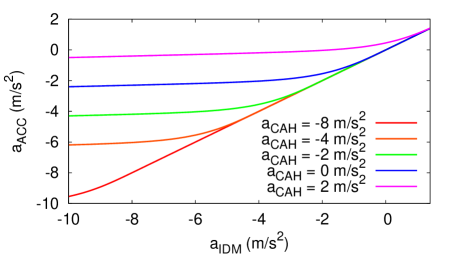
Figure 2: Resulting acceleration $a_{\text{ACC}}$ of the ACC model, equation (4), as a function of the IDM acceleration for different values of the acceleration $a_{\text{CAH}}$ resulting from the constant-acceleration heuristic (CAH).

2.4 Simulating the Properties of the ACC Model

Figure 3 displays simulations of a mildly critical ‘cut-in’ situation: Another vehicle driving at the same velocity 80 km/h merges at time $t=0$ in front of the ACC vehicle (car parameters of table 1) resulting in an initial gap $s(0)=10\,\mathrm{m}$. Although the corresponding time headway $s(0)/v(0)=0.45\,\mathrm{s}$ is less than one third of the desired minimum time headway $T=1.5\,\mathrm{s}$, the situation is not really critical because the approaching rate at the time of the lane change is zero (the time-to-collision $s/\Delta v$ is even infinite). Consequently, the ACC model results in a braking deceleration that does not exceed the comfortable deceleration $b=2\,\mathrm{m/s^{2}}$. In contrast, the IDM leads to decelerations reaching temporarily the maximum value assumed to be physically possible ($8\,\mathrm{m/s^{2}}$). In spite of the more relaxed reaction, the velocity drop of the ACC vehicle is slightly less than that of the IDM (minimum velocities of about 69 km/h and 68 km/h, respectively).

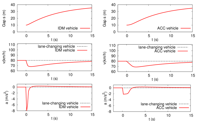
Figure 3: Response of an IDM and an ACC vehicle (‘car’ parameters of table 1) to the lane-changing manoeuvre of another vehicle immediately in front of the considered vehicle. The initial velocities of both vehicles is 80 km/h, and the initial gap is 10 m. This can be considered as a ‘mildly critical’ situation.

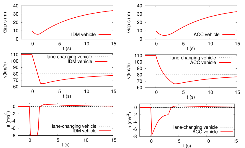
Figure 4: Response of an IDM and an ACC vehicle to an abrupt lane-changing manoeuvre of another vehicle immediately in front of the considered vehicle. The decelerations are restricted to $8\,\mathrm{m/s^{2}}$. The initial velocity of the lane-changing vehicle is 80 km/h, while the initial velocity of the considered vehicle is 110 km/h. This is a ‘strongly critical’ situation.

A seriously critical situation is depicted in figure 4. While the ‘cut-in’ results in the same initial gap $s(0)=10\,\mathrm{m}$ as in the situation discussed above, the ACC vehicle is approaching rapidly (initial approaching rate $\Delta v(0)=30\,\mathrm{km/h}$) and an emergency braking is mandatory to avoid a rear-end crash. For this case, the reactions of the two models are similar. Both the IDM and the ACC models lead to initial decelerations near the maximum value. However, the deceleration of the ACC vehicle quickly decreases towards the comfortable deceleration before reverting to a stationary situation. In contrast, the IDM vehicle remains in emergency mode for nearly the whole braking manoeuvre. Of course, the more relaxed ACC behaviour leads to a closer minimum gap (4 m compared to 5.5 m for the IDM). Nevertheless, the velocity drop of the ACC vehicle is slightly lower than that of the IDM (minimum velocities of about 66 km/h compared to 64 km/h).

Both the maximum deceleration and the velocity drop are measures for the perturbations imposed on following vehicles and therefore influence the stability of a platoon of vehicles, i.e., the ‘string stability’. While softer braking reactions generally lead to a reduced string stability, the reduced perturbations behind ACC vehicles generally compensate for this effect. In fact, figure 5 shows for a specific example, that the excellent stability properties of the IDM carry over to the ACC model. Further simulations show that, for the ‘car’ model parameter set of table 1 and also for heterogeneous traffic composed of up to 40% trucks, string stability is satisfied for nearly all situations. An analytical investigation to delineate the stability limits is the topic of future work.

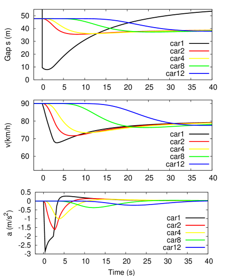
Figure 5: Response of a platoon of ACC vehicles to an abrupt lane-changing manoeuvre of another vehicle ($v=80\,\mathrm{km/h}$) in front of the platoon with an initial gap of 10 m only. The desired velocity of the platoon leader is 90 km/h, while that of the followers is 120 km/h.

3 Driving Strategy for Adaptive Cruise Control Systems

In this section we summarize an extension of adaptive cruise control (ACC) systems towards traffic-condition-dependent driving strategies, which has recently been proposed by the authors [Kesting et al., 2008]. Since drivers require to have full control of and confidence in their car, an ACC system should be designed in a way that its driving characteristics is similar to the natural driving style of human drivers. In order to nevertheless improve traffic performance by automated driving, we therefore propose a traffic-adaptive driving strategy which can be implemented by changing the model parameters depending on the local traffic situation.

For an efficient driving behaviour it is sufficient to change the default driving behaviour only temporarily in specific traffic situations. The situations in which the parameters are dynamically adapted have to be determined autonomously by the equipped vehicle [Kesting et al., 2008]. To this end, we consider the following discrete set of five traffic conditions that are characterized as follows:

1. Free traffic. This is the default situation. The ACC settings are determined solely by the maximum individual driving comfort. Since each driver can set his or her own parameters for the time gap and the desired speed, this may lead to different settings of the ACC systems.

2. Upstream jam front. Here, the objective is to increase safety by reducing velocity gradients. Compared to the default situation, this implies earlier braking when approaching slow vehicles. Note that the operational layer always assures a safe approaching process independent of the detected traffic state.

3. Congested traffic. Since drivers cannot influence the development of traffic congestion in the bulk of a traffic jam, the ACC settings are reverted to their default values.

4. Downstream jam front. To increase the dynamic bottleneck capacity, accelerations are increased and time gaps are temporarily decreased.

5. Bottleneck sections. Here, the objective is to locally increase the capacity, i.e., to dynamically bridge the capacity gap. This requires a temporary reduction of the time gap. Moreover, by increasing the maximum acceleration, the string stability of a vehicle platoon is increased due to a shorter adaptation time to changes in the velocities [Kesting & Treiber, 2008b].

Each traffic condition can be associated with certain settings for the model parameters implementing the intended driving style. For the enhanced Intelligent Driver Model (cf. §2), the relevant parameters are the desired time gap $T$, the desired maximum acceleration $a$, and the desired deceleration $b$. In order to preserve the individual settings of the drivers or users, respectively, changes in the parameter sets for each traffic state can be formulated in terms of multiplication factors. These relative factors $\lambda$ can be arranged in a ‘driving strategy matrix’ shown in table 2. For example, $\lambda_{T}=0.7$ denotes a reduction of the default time gap $T$ by 30% in bottleneck situations.

Table 2: Summary of the ACC driving strategies

Each of the traffic conditions corresponds to a different set of ACC control parameters. The ACC driving characteristics are represented by the IDM parameters safety time gap $T$, the maximum acceleration $a$ and the comfortable deceleration $b$. $\lambda_{T}$, $\lambda_{a}$, and $\lambda_{b}$ are multiplication factors.

Traffic condition	$\quad\lambda_{T}\quad$	$\quad\lambda_{a}\quad$	$\quad\lambda_{b}\quad$	Driving behaviour
Free traffic	1	1	1	Default/Comfort
Upstream front	1	1	0.7	Increased safety
Congested traffic	1	1	1	Default/Comfort
Downstream front	0.5	2	1	High dynamic capacity
Bottleneck	0.7	1.5	1	Breakdown prevention

As indicated in the strategy matrix, the default settings (corresponding to $\lambda=1$) are used most of the time. For improving traffic performance, only two traffic states are relevant. The regime ‘passing a bottleneck section’ aims at an suppression (or, at least, at a delay) of the traffic flow collapse by lowering the time gap $T$ in combination with an increased acceleration $a$. Furthermore, a short-term reduction of traffic congestion can only be obtained by increasing the outflow. This is the goal in the traffic condition ‘downstream jam front’, aiming at a brisk leaving of the queue by increasing the maximum acceleration $a$ and decreasing the safe time gap $T$ of the ACC system. Both regimes are systematically evaluated in the following section.

4 Impact of the ACC Driving Strategies on Capacities

In this section we investigate the impact of ACC-equipped vehicles implementing the traffic-adaptive driving strategy on the traffic performance by systematically varying the given ACC proportion. The philosophy of our simulation approach is to control the system by keeping as many parameters constant (ceteris paribus methodology). Consequently, we start with a well defined system (with 0% ACC) and vary the ACC fraction as external parameter. In free flow, the maximum throughput of a freeway is determined by the maximum flow occurring before the traffic flow breaks down, while in congested traffic it is given by the dynamic capacity (i.e., the outflow from a traffic jam). These capacities will be studied in §4 (4.1) and §4 (4.2).

4.1 Maximum Flow in Free Traffic

The relevant measure for assessing the efficiency of the proposed driving strategy ‘passing a bottleneck section’ is the maximum possible flow until the traffic flow breaks down. An upper bound for this quantity $C$, defined as the maximum number of vehicles per unit time and lane capable of passing the bottleneck, is given by the inverse of the safe time gap $T$, i.e., $C<1/T$. However, the theoretical maximum flow also depends on the effective length $l_{\text{eff}}=l+s_{0}$ of a driver-vehicle unit (which is given by the vehicle length $l$ plus the minimum bumper-to-bumper distance $s_{0}$). Therefore, the theoretically possible maximum flow is

$$Q_{\text{max}}^{\text{theo}}=\frac{1}{T}\left(1-\frac{l_{\text{eff}}}{v_{0}T+l_{\text{eff}}}\right).$$ (5)

This static road capacity $Q_{\text{max}}^{\text{theo}}$ corresponds to the maximum of a triangular fundamental diagram. In the case of the IDM (with a finite acceleration), the theoretical maximum is even lower [Treiber et al., 2000]. Generally, the maximum free flow $Q_{\text{max}}^{\text{free}}$ before traffic breaks down is a dynamic quantity that depends on the traffic stability as well. Typically, we have $Q_{\text{max}}^{\text{free}}\leq Q_{\text{max}}^{\text{theo}}$.

In the following, we will therefore analyse the maximum free flow $Q_{\text{max}}^{\text{free}}$ resulting from traffic simulations. To this end, we consider a simulation scenario with a two-lane freeway and an on-ramp which creates a bottleneck situation. The lane-changing decisions have been modelled using MOBIL [Kesting et al., 2007]. The inflow at the upstream boundary was increased with a constant rate of $\dot{Q}=700\,\mathrm{veh/h^{2}}$, while the ramp flow was kept constant at 250 veh/h/lane. We have checked other progression rates as well, but only found a marginal difference. In order to determine the maximum free flow, we have used the following criterion: A traffic breakdown is detected, if more than 20 vehicles on the main road drive slower than $v_{\text{crit}}=30\,\mathrm{km/h}$. After a traffic breakdown has been detected, we use the flow of the actual 1-min aggregate of a ‘virtual’ detector located downstream of the on-ramp to measure the maximum flow.

4.1.1 Probability of a breakdown of traffic flow

The maximum free flow $Q_{\text{max}}^{\text{free}}$ results from a measurement process which is based on 1-min aggregation intervals. As the underlying complex traffic simulation involves nonlinear models, discrete lane change decisions, random influences (such as the vehicle type inserted at the upstream boundary etc.), it is expected that $Q_{\text{max}}^{\text{free}}$ is a stochastically varying quantity, leading to different measurements even for identical boundary and initial conditions (assuming a random seed of the computer’s pseudo-random number generator). Consequently, we will consider the maximum free flow as a random variable which reflects the probabilistic nature of a traffic flow breakdown [Brilon et al., 2007; Kerner, 2004; Persaud et al., 1998].

The statistical properties of $Q_{\text{max}}^{\text{free}}$ have been investigated by means of repeated simulation runs. We have examined scenarios with a total truck percentage of 10% with an additional ACC equipment level of 20% and without ACC-equipped vehicles. Furthermore, we have considered inter-driver variability by assigning uniformly and independently distributed values to the IDM parameters $v_{0}$, $T$, $a$ and $b$, where the averages of the parameter values have been left unchanged, while the width of the distributions have been set to 20% (i.e., the individual values vary between 80% and 120% of the average parameter value). Each scenario has been simulated 1000 times to derive the statistical properties of the maximum free flow. The resulting cumulative distribution functions for $Q_{\text{max}}^{\text{free}}$, reflecting the probability of a traffic flow breakdown, are shown in figure 6. As the measurement of the maximum free flow yields a distribution of finite variance and results from many stochastic contributions, the resulting cumulative distribution function is expected to follow the Central Limit Theorem. In fact, the integrated (and normalized) Gaussian function $N(x;\mu,\sigma^{2})$ with mean value $\mu$ and variance $\sigma^{2}$ fits the simulation results well.

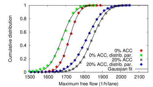
Figure 6: Traffic breakdown probability for an ACC equipment rate of 0% and 20%, respectively, and for different degrees of heterogeneity. The diagrams show the cumulative distribution functions of the maximum free flow, resulting from 1000 simulation runs and numerical fits for the Gaussian distribution.

From the results in figure 6, we draw the following conclusions: First, an increased proportion of ACC vehicles shifts the maximum throughput to a larger mean value. This shows the positive impact of the traffic-adaptive driving strategy on the traffic efficiency. In particular, the temporary change of the driving characteristics while passing the bottleneck helps to increase the maximum throughput by 6–8% in the considered scenarios (at an ACC equipment level of $\alpha=20\%$).

Second, the considered traffic scenarios show different degrees of heterogeneity, i.e., mixtures of various vehicle types (cars and trucks, equipped with ACC system or not) and statistically distributed model parameters. An increase in the degree of heterogeneity leads to larger fluctuations in the traffic flow which, in turn, results in a larger variation $\sigma$ of the random variable $Q_{\text{max}}^{\text{free}}$ and also in a slightly reduced mean value.

Third, as the consideration of ACC-equipped vehicles with their adaptive (i.e., time-dependent) parameter choice increases the level of heterogeneity in a significant way, the variation $\sigma$ is increased compared to the values without ACC vehicles. This finding makes clear that the impact of ACC-equipped vehicles on the traffic dynamics must be studied with a realistic level of heterogeneity, e.g., in a multi-lane freeway scenario considering cars and trucks. Otherwise, the assessment of ACC systems may erroneously lead to discouraging (or overly optimistic) results.

4.1.2 Maximum free flow as a function of the ACC proportion

Let us now investigate the maximum free flow as a function of the ACC proportion $\alpha$. To this end, we have gradually increased $\alpha$ in a range from $0$ to $50\%$, using the scenario described above. In figure 7, the result of each simulation run is represented by one point. As expected from our previous findings, the values of the maximum free flow $Q_{\text{max}}^{\text{free}}$ vary stochastically. For better illustration, we have therefore used a kernel-based linear regression, which calculates the expectation value and the standard deviation as a continuous function of $\alpha$. The only parameter of this evaluation procedure is the width $\delta$ of the smoothing kernel. Here, we have used $\delta=0.1$. Details of the numerical method are described in 5.

Figure 7(a) shows the results for a traffic scenario without trucks and a scenario with $10\%$ trucks. As expected, increasing the proportion of trucks with their higher safe time gap $T$ (cf. table 1) reduces the maximum free flow. However, the average value of the maximum free flow increases with growing ACC equipment level $\alpha$. The gain in the maximum free flow is basically proportional to $\alpha$.

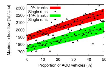
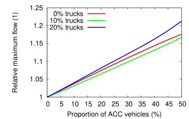
Figure 7: Maximum free flow until traffic breaks down as a function of the ACC proportion for various truck fractions. Note that the genuine cumulative distributions for $\alpha=0\%$ and $\alpha=20\%$ are shown in figure 6.

Figure 7(b) summarizes the simulation results for various truck proportions in terms of the relative increase $q_{\text{max}}^{\text{free}}=Q_{\text{max}}^{\text{free}}(\alpha)/Q_{\text{max}}^{\text{free}}(0)$ of the maximum flow compared to situations with non-equipped vehicles. This quantity allows for a direct comparison between the different simulation scenarios. For example, the gain in the maximum free flow varies between approximately 16% and 21% for an ACC fraction of 50%. For an ACC portion of 20%, the maximum free flow increases by approximately 7%. Although this appears to be a relatively small enhancement, one should not underestimate its impact on the resulting traffic dynamics. The authors, for example, have shown that an ACC proportion of 20% can often prevent (or, at least, delay) a breakdown of traffic flow [Kesting et al., 2008]. Comparing this to the reference simulation without ‘intelligent’ ACC-equipped vehicles, individual travel times vary by a factor of 2 or 3 at least, sometimes even more. As the gain in the maximum free flow is basically proportional to $\alpha$, the quantity $q_{\text{max}}^{\text{free}}/\alpha$ is approximately constant and describes the relative gain in $Q_{\text{max}}^{\text{free}}$ per ACC portion $\alpha$. The values for the simulation results shown in figure 7 are in the range between $0.32$ and $0.42$.

4.1.3 Maximum flow for different driving strategy parameters

Besides the proportions of trucks and ACC-equipped vehicles, the traffic performance is influenced by the multiplication factors $\lambda$ of the ACC driving strategy in the bottleneck state. In particular, the maximum free flow depends on the modification $\lambda_{T}$ of the time gap and $\lambda_{a}$ of the maximum acceleration in the ‘bottleneck condition’. As default values, we have chosen $\lambda_{T}^{\text{bottle}}=0.7$ and $\lambda_{a}^{\text{bottle}}=1.5$ (see table 2). While considering the aforementioned simulation scenario with 10% trucks, we have varied these driving strategy parameters in the ‘bottleneck’ state as shown in figure 8.

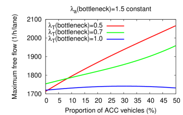
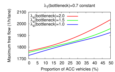
Figure 8: Average maximum free flow as a function of the ACC proportion for the simulation scenario with 10% trucks. The ACC driving strategy in the ‘bottleneck’ state is varied: The left diagram shows various settings for $\lambda_{T}$ while keeping the maximum acceleration $a$ constant. The right diagram refers to simulation results for various values of $\lambda_{a}$, while the safe time gap $T$ is kept constant.

The left diagram in figure 8 shows the strong impact of the safe time gap $T$ on the maximum free flow (while keeping $\lambda_{a}^{\text{bottle}}=1.5$ constant). A further reduction of the ACC time gap with $\lambda_{T}=0.5$ leads to a stronger increase in the maximum free flow when considering a growing ACC proportion. Note that this is consistent with equation (5). Moreover, the modification of $a$ alone while keeping $T$ unchanged ($\lambda_{T}=1$) does not improve the maximum free flow.

The maximum acceleration $a$ has clearly a smaller effect on the maximum free flow than $T$, as displayed in the right diagram of figure 8. While keeping $\lambda_{T}$ constant, different settings such as $\lambda_{a}=1$, $1.5$ or $2$ do not change the resulting maximum free flow in a relevant way. So, the throughput can only be efficiently increased in combination with smaller time gaps (corresponding to lower values of $\lambda_{T}$).

4.2 Dynamic Capacity after a Traffic Breakdown

Let us now investigate the system dynamics after a breakdown of traffic flow. Traffic jam formation is determined by the difference of the upstream inflow $Q_{\text{in}}$ and the outflow $Q_{\text{out}}$ from the downstream jam front (i.e., the head of the queue) which is also called dynamic capacity. We use the same simulation setup (of a two-lane freeway with an on-ramp) as in the previous section. Whenever a traffic breakdown was provoked by the increasing inflow, we aggregated the flow data of the ‘virtual detector’ $1\,$km downstream of the bottleneck within an interval of 10 minutes.

4.2.1 Dynamic capacity as a function of the ACC proportion

Figure 9(a) shows the resulting dynamic capacity for a variable percentage of ACC vehicles in a scenario without trucks and in a scenario with 10% trucks. Single simulation runs are depicted by symbols, while the average and the variation band were calculated from the scattered simulation data via the kernel-based linear regression using a width of $\delta=0.1$ (cf. 5). As intended by the proposed traffic condition ‘downstream jam front’, the dynamic capacity increases with growing ACC equipment rate.

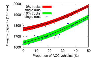
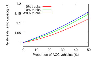
Figure 9: Dynamic capacity as a function of the percentage of ACC vehicles. The outflow from a traffic jam increases with a growing proportion of ACC-equipped vehicles due to the changed driving strategy for the ‘downstream jam front’ condition.

Figure 9(b) compares the results for different truck proportions by considering the relative increase of the dynamic capacity $q_{\text{out}}(\alpha)=Q_{\text{out}}(\alpha)/Q_{\text{out}}(0)$ with the ACC equipment level $\alpha$. For $\alpha=50\%$, the relative increase of $q_{\text{out}}$ is between 12% and 16% and therefore somewhat lower than the increase of the maximum free capacity (cf. §4 (4.1). Interestingly, the dynamic capacity does not increase linearly as the measured maximum free capacity displayed in figure 7, but faster. Consequently, the relative increase $q_{\text{out}}(\alpha)$ grows over-proportionally with higher ACC equipment rates $\alpha$. This can be understood by an ‘obstruction effect’ caused by slower accelerating drivers (in particular, trucks) which hinder faster (ACC) vehicles.

Furthermore, we can compare the maximum free capacity $Q_{\text{max}}^{\text{free}}$ displayed in figure 7 with the dynamic capacity $Q_{\text{out}}$, which is lower than $Q_{\text{max}}^{\text{free}}$. The difference between both quantities is referred to as capacity drop. Notice that the capacity drop is the crucial quantity determining the performance (loss) of the freeway under congested conditions and accounts for the persistence of traffic jams once the traffic flow has broken down. Realistic values for the capacity drop are between 5% and 20% [Kerner & Rehborn, 1996; Cassidy & Bertini, 1999]. In our simulations, we found that the values of the relative capacity drop are typically between 5 and 15%.

4.2.2 Dynamic capacity for different driving strategy parameters

The increase of the dynamic capacity is based on the proposed driving strategy for the traffic condition ‘downstream jam front’. The ACC-equipped vehicles increase their maximum acceleration $a$ in combination with a decrease in the time gap $T$ (cf. table 2). In figure 10, simulation results are shown for various multiplication factors $\lambda_{a}$ and $\lambda_{T}$ for the traffic condition ‘downstream jam front’ (using a scenario with 10% trucks). The default values $\lambda_{a}^{\text{down}}=2$ and $\lambda_{T}^{\text{down}}=0.5$ correspond to the results shown in figure 9. The simulation results demonstrate that the dynamic capacity is only increased in a relevant way by adapting $a$ and $T$ simultaneously.

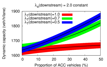
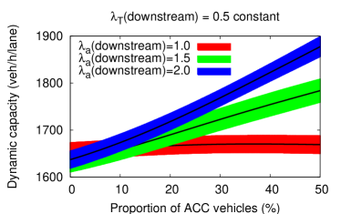
Figure 10: Dynamic capacity for various multiplication factors $\lambda$ used by the simulated ACC system in the ‘downstream jam front’ traffic condition. The results show that the dynamic capacity is increased in a relevant way only by adapting $a$ in combination with $T$.

5 Discussion

In view of an increasing number of vehicles equipped with adaptive cruise control (ACC) systems in the future, it is important to address questions about their impact and potentials on the collective traffic dynamics. Until now, microscopic traffic models have mainly been used to (approximately) describe the human driver. For a realistic description of the future mixed traffic, however, appropriate models for both human driving and automated driving are needed. Car-following models reacting only to the preceding vehicle have originally been proposed to describe human drivers, but, from a formal point of view, they describe more closely the dynamics of ACC-driven vehicles. Thus, we have considered the simple yet realistic Intelligent Driver Model (IDM) [Treiber et al., 2000] as a starting point for an adequate description of the driving behaviour on a microscopic level. The IDM, however, is intended to describe traffic dynamics in one lane only, and leads, e.g. in lane-changing situations, to unrealistic driving behaviour when the actual gap is significantly lower than the desired gap. For such situations, we have formulated an alternative heuristic based on the assumption of constant accelerations in order to prevent unnaturally strong braking reactions due to lane changes. The proposed enhanced IDM combines the well-proven properties of the original model with this constant-acceleration heuristic resulting in a more relaxed driving behaviour in situations with are typically not considered to be critical by human drivers. The new acceleration function (4) depends (besides gap and velocity) additionally on the acceleration of the leading vehicle.

Since the enhanced IDM is still a car-following model, we have called it ‘ACC model’. In fact, it has already been implemented (with some further confidential extensions) in real test cars showing a realistic and natural driving dynamics [Kranke & Poppe, 2008; Kranke et al., 2006]. This consistency between automated driving and the ‘driving experience’ of humans can be considered as a key account for the acceptance of and the confidence in ACC systems. Moreover, since the driver is obliged to override the ACC system at any point in time, an automated driving characteristics similar to those of human drivers is a safety-relevant premise. Hence, a realistic car-following, i.e., an ACC model can be considered also as a appropriate description of the human driving although humans’ perceptions and reactions fundamentally differ from those of ACC systems [Treiber et al., 2006].

The proposed ACC-model has been used to evaluate potentials of a vehicle-based approach for increasing traffic performance in a mixed system consisting of human drivers and ACC systems. While human drivers of cars and trucks have been modelled with constant model parameters, the proposed adaptation of the driving style according to the actual traffic conditions corresponds to parameters that vary over time. Note that the concrete meanings of the IDM parameters allow for direct implementations of the considered driving strategies.

By means of multi-lane traffic simulations, we have investigated the maximum free flow before traffic breaks down (as crucial quantity in free traffic), and the dynamic capacity (which determines as outflow from a traffic jam the dynamics in congested traffic) by systematically increasing the fraction of vehicles implementing multiple driving strategies. For the maximum free flow, we found an approximately linear increase with a sensitivity of about $0.3\%$ per 1% ACC fraction. The dynamic capacity shows a non-linear relationship with an increase of about 0.24% per 1% ACC fraction for small equipment rates. Both quantities can be considered as generic measures for the system performance. These sensitivities multiply when considering other relevant measurements like travel times resulting in large variations by factors of 2-4 [Kesting et al., 2008]. The presented results reveal the (positive) impact of the driving behaviour on traffic dynamics even when taking into consideration the idealized assumptions and conditions in traffic simulations.

Finally, we note that the in-vehicle implementation of traffic-adaptive driving strategies and the detection of the proposed traffic conditions in real-time are investigated in ongoing research projects. Different technologies such as specifically attributed maps [Kesting et al., 2008], inter-vehicle communication [Thiemann et al., 2008; Kesting et al., 2009], and vehicle-infrastructure integration [Kranke & Poppe, 2008] are considered at present.

Kernel-Based Linear Regression When dealing with simulations, one often varies a single model parameter and plots over it a second quantity that results from the related simulation run. Here, a statistical method is presented that combines the gradual change in the independent model parameter $x$ with the estimation of the standard deviation in the resulting fluctuating quantity $y$ without running multiple simulations for the same parameter value $x$.

Suppose we are fitting $n$ data points $\{x_{i},y_{i}\},\,i=1,\ldots,n$ to a linear model with two parameters $a$ and $b$, $\hat{y}(x)=a+bx$. A global measure for the goodness of fit is the sum of squared errors $y_{i}-\hat{y}(x_{i})$. The best-fitting curve for the linear regression can be obtained by the method of least squares with respect to the fit parameters $a$ and $b$. The solution of the system of linear equations is given by

$$b=b(\{x_{i},y_{i}\}) = \frac{\langle xy\rangle-\langle x\rangle\langle y\rangle}{\langle x^{2}\rangle-\langle x\rangle^{2}},$$ (6)

$$a=a(\{x_{i},y_{i}\}) = \frac{\langle x^{2}\rangle\langle y\rangle-\langle x\rangle\langle xy\rangle}{\langle x^{2}\rangle-\langle x\rangle^{2}},$$ (7)

where the arithmetic average $\langle z\rangle$ of the measured data points $\{z_{i}\}$ is defined by $\langle z\rangle:=\frac{1}{n}\sum_{i=1}^{n}z_{i}$. Let us now generalize the linear regression by using a locally weighted average

$$\langle z\rangle(x):=\sum_{i=1}^{n}w(x-x_{i})\,z_{i},$$ (8)

where the weights $w(x-x_{i})$ are defined through a sufficiently localized function $K$ with $w(x-x_{i})={K(x-x_{i})}/\sum_{j}K(x-x_{j})$. As the expression (8) is evaluated locally for any value $x$, the dependence on $x$ is transferred to the linear fit parameters (6) and (7). For plotting $y$ against $x$, the special case of centering the averages at $x^{\prime}=x$ is relevant. With $a(x)=\langle y\rangle(x)-b(x)\,x$, we obtain

$$\hat{y}(x,x)=a(x)+b(x)\,x=\langle y\rangle(x).$$ (9)

Furthermore, the residual error $y_{i}-\hat{y}(x_{i})$ is also weighted by the discrete convolution (8), resulting in

$$\sigma^{2}(x)=\sum_{i=1}^{n}w_{i}(x)\left[y_{i}-a(x)-b(x)x_{i}\right]^{2}.$$ (10)

Notice that the ‘error band’ $\sigma(x)$ describes the variations of the quantity $y$ on length scales smaller than the width of the smoothing kernel $K$. For stochastic simulations, this is simultaneously an estimate of the fluctuations for given values of $x$. In this paper, we use a Gaussian kernel $K(x)=\exp\left[-x^{2}/(2\delta^{2})\right]$ as weight function. The width of the Gaussian kernel $\delta$ is the only parameter of the kernel-based linear regression.

References

- Brilon et al. [2007] Brilon, W., Geistefeldt, J. & Zurlinden, H. 2007 Implementing the Concept of Reliability for Highway Capacity Analysis. Transportation Research Record, 2027, 1–8.
- Brockfeld et al. [2004] Brockfeld, E., Kühne, R. D. & Wagner, P. 2004 Calibration and validation of microscopic traffic flow models. Transportation Research Record, 1876, 62–70.
- Cassidy & Bertini [1999] Cassidy, M. J. & Bertini, R. L. 1999 Some traffic features at freeway bottlenecks. Transportation Research Part B: Methodological, 33, 25–42.
- Davis [2004] Davis, L. 2004 Effect of adaptive cruise control systems on traffic flow. Physical Review E, 69, 066 110.
- Helbing [2001] Helbing, D. 2001 Traffic and related self-driven many-particle systems. Reviews of Modern Physics, 73, 1067–1141.
- Helbing et al. [2009] Helbing, D., Treiber, M., Kesting, A. & Schönhof, M. 2009 Theoretical vs. empirical classification and prediction of congested traffic states. The European Physical Journal B, 69, 583–598.
- Kerner & Rehborn [1996] Kerner, B. & Rehborn, H. 1996 Experimental features and characteristics of traffic jams. Physical Review E, 53, R1297–R1300.
- Kerner [2004] Kerner, B. S. 2004 The physics of traffic: Empirical freeway pattern features, engineering applications, and theory. Springer.
- Kesting & Treiber [2008a] Kesting, A. & Treiber, M. 2008a Calibrating car-following models by using trajectory data: Methodological study. Transportation Research Record, 2088, 148–156.
- Kesting & Treiber [2008b] Kesting, A. & Treiber, M. 2008b How reaction time, update time and adaptation time influence the stability of traffic flow. Computer-Aided Civil and Infrastructure Engineering, 23, 125–137.
- Kesting et al. [2007] Kesting, A., Treiber, M. & Helbing, D. 2007 General lane-changing model MOBIL for car-following models. Transportation Research Record, 1999, 86–94.
- Kesting et al. [2009] Kesting, A., Treiber, M. & Helbing, D. 2009 Connectivity statistics of store-and-forward inter-vehicle communication. IEEE Transactions of Intelligent Transportation Systems. in print.
- Kesting et al. [2008] Kesting, A., Treiber, M., Schönhof, M. & Helbing, D. 2008 Adaptive cruise control design for active congestion avoidance. Transportation Research Part C: Emerging Technologies, 16(6), 668–683.
- Kranke & Poppe [2008] Kranke, F. & Poppe, H. 2008 Traffic guard - merging sensor data and C2I/C2C information for proactive congestion avoiding driver assistance systems. In FISITA World Automotive Congress.
- Kranke et al. [2006] Kranke, F., Poppe, H., Treiber, M. & Kesting, A. 2006 Driver assistance systems for active congestion avoidance in road traffic (in German). In VDI-Berichte zur 22. VDI/VW Gemeinschaftstagung: Integrierte Sicherheit und Fahrerassistenzsysteme (ed. M. Lienkamp), vol. 1960, p. 375. Association of German Engineers (VDI).
- Marsden et al. [2001] Marsden, G., McDonald, M. & Brackstone, M. 2001 Towards an understanding of adaptive cruise control. Transportation Research Part C: Emerging Technologies, 9, 33–51.
- Ossen & Hoogendoorn [2005] Ossen, S. & Hoogendoorn, S. P. 2005 Car-following behavior analysis from microscopic trajectory data. Transportation Research Record, 1934, 13–21.
- Ossen et al. [2007] Ossen, S., Hoogendoorn, S. P. & Gorte, B. G. 2007 Inter-driver differences in car-following: A vehicle trajectory based study. Transportation Research Record, 1965, 121–129.
- Panwai & Dia [2005] Panwai, S. & Dia, H. 2005 Comparative evaluation of microscopic car-following behavior. IEEE Transactions on Intelligent Transportation Systems, 6(3), 314–325.
- Persaud et al. [1998] Persaud, B., Yagar, S. & Brownlee, R. 1998 Exploration of the breakdown phenomenon in freeway traffic. Transportation Research Record, 1634, 64–69.
- Punzo & Simonelli [2005] Punzo, V. & Simonelli, F. 2005 Analysis and comparision of microscopic flow models with real traffic microscopic data. Transportation Research Record, 1934, 53–63.
- Thiemann et al. [2008] Thiemann, C., Treiber, M. & Kesting, A. 2008 Longitudinal hopping in inter-vehicle communication: Theory and simulations on modeled and empirical trajectory data. Phyical Review E, 78, 036 102.
- Treiber et al. [2000] Treiber, M., Hennecke, A. & Helbing, D. 2000 Congested traffic states in empirical observations and microscopic simulations. Physical Review E, 62, 1805–1824.
- Treiber et al. [2006] Treiber, M., Kesting, A. & Helbing, D. 2006 Delays, inaccuracies and anticipation in microscopic traffic models. Physica A, 360, 71–88.
- van Arem et al. [2006] van Arem, B., van Driel, C. & Visser, R. 2006 The impact of cooperative adaptive cruise control on traffic-flow characteristics. IEEE Transactions on Intelligent Transportation Systems, 7(4), 429–436.
- VanderWerf et al. [2002] VanderWerf, J., Shladover, S., Miller, M. & Kourjanskaia, N. 2002 Effects of adaptive cruise control systems on highway traffic flow capacity. Transportation Research Record, 1800, 78–84.